EU$N$HA: a New Cosmological Hydro Simulation Code

1 Introduction

Over the last few decades, state-of-the-art cosmological $N$-body simulation (Kim et al., 2009, 2011; Rasera et al., 2013; Angulo et al., 2012; Kuhlen, et al., 2012) has proven to be a powerful tool for study of the Large-scale Structures (LSS) of the Universe. The observed distribution of galaxies is well reproduced by the $N$-body dynamics in terms of the two-point correlations (Masaki et al., 2013) or power spectrum of galaxies (Tegmark et al., 2006), cosmic topology (Choi et al., 2010, 2013), and the abundance of groups (Nurmi et al., 2013) or the largest structure in the universe (Park et al., 2012). These statistical studies enable us to refine the current cosmological model by constraining model parameters at the percent level of accuracy.

Below the galaxy scale, however, hydrodynamics begin to dominate gravitational forces. In the potential well of a dark matter halo, baryonic matter decouples from the surrounding dark matter inflow forming distinct and complex inner structures such as galactic disks, bulges, spiral arms, and so on. Therefore, it would be indispensable to include the hydrodynamical effects if one wants to study galaxy formation and evolution.

The Two Degree Field Galaxy Redshift Survey (2dFGRS; Colless et al. 2001) and a series of the Sloan Digital Sky Survey (SDSS; Aihara et al. 2011), for example, have enabled us to study physical properties of and the environmental effect on individual galaxies. In the current paradigm of hierarchical clustering, it is believed that a galaxy is a aggregate of the merging of smaller objects. Therefore, the secular evolution of a galaxy and interaction between galaxies began to be investigated in great detail in the cosmological context. Park & Hwang (2009) reported that the morphology of a galaxy is correlated with that of the nearest neighbors. This correlation maybe reasonably attributed to hydrodynamic interactions between the galaxy and its neighbors.

An observed galaxy is an accumulated sum of various physical processes over a long period of time. Galaxies have been shaped not only by gravity and hydrodynamic forces but also by other astrophysical processes like cooling, heating, star formation, and supernova feedback. Baryonic matter is believed to settle down in the deep potential wells of dark matter and stars form therein, in high density environments. After consuming all available fuel by nuclear fusion, massive stars at last explode as supernovae dispersing energy and metal-enriched material into the interstellar medium. This explosion may trigger another star formation, and so the baryonic component starts another life cycle of metal enrichment. Consequently, the new generation of stars has higher metallicity than before. Therefore, a galaxy may have a wide spectrum of stellar populations and metallicities.

There are many cosmological hydrodynamic simulation codes available today (Kravtsov, 1999; Fryxell et al., 2000; Teyssier, 2002; O’Shea et al., 2004; Wadsley, Stadel, & Quinn, 2004; Springel, 2005; Wetzstein et al., 2009; Springel, 2010, among others). Largely, they can be grouped in two categories; Eulerian and Lagrangian codes. The Eulerian scheme use regular grids to compute the hydrodynamic interaction between grids. However, the Lagrangian code is based on the particles carrying the hydrodynamic properties. Mutual interactions between particles are computed using the SPH (smoothed particle hydrodynamics).

The GOTPM (Dubinski et al., 2004) code is especially well designed for massive $N$-body simulations with an efficient use of memory space and fast calculation speeds. For example, the Horizon-Runs (HRs; Kim et al. 2009, 2011), which were the largest ones at that time, were performed with $70-350$ billion particles. The GOTPM code adopts non-recursive walks on oct-sibling tree structures which speeds up the code significantly.

On top of the GOTPM code, we placed the SPH algorithms to properly simulate cosmological structures down to the galaxy scale the hydrodynamic forces are more dominant than the gravity. Among the SPH algorithms, we adopt the entropy-conservation scheme (Springel, 2005). We used the CLOUDY 90 package (Ferland et al., 1998) to arrange a table of the heating and cooling rates for reference during the simulation run. We set a global value for the reionization epoch and the heating rated before and after reionization are different. After reionization, Jeans’s mass may increase and small mass objects are prevented from forming due to baryonic pressure resisting gravitational contraction. We include the self-shielding of gas particles from uniform UV backgrounds, which may have a larger effect on the formation of the dwarf galaxies in the early universe (Tajiri & Umemura, 1998; Sawala et al., 2010).

This paper is organized as follows: In Section 2, we present the basic equation of motion of the $N$-body particles. The hydrodynamic equations are listed in Section 3. Section 4 is devoted to a description of the individual time stepping adopted in the code and Section 5 shows how to implement astrophysical processes in the code. Simulation tests and the results are discussed in Section 6. We summarize our work in Section 7.

2 Basic Equations of Motion

In an expanding background, the comoving distance ($\mathbf{x}$) is related to the physical distance ($\mathbf{r}$) with the scale factor ($a$) as

$$\mathbf{r} = {a\over a_{m}}\mathbf{x},$$ (1)

where $a_{m}$ is the maximum value of the scale factor or the scale factor at $z=0$. In the GOTPM code, we use the following variables

$$\mathbf{x} = {\ell_{b}\over a_{m}}{\mathbf{x}}_{s},$$ (2)

$$m_{r} = \ell_{b}^{3}\left<\rho_{0}\right>m_{s},$$ (3)

where ${\mathbf{x}}_{s}$ is the position of the particle in unit of the mean particle separation ($\ell_{b}\equiv L_{b}/N$), $L_{b}$ is the simulation box size on one side, $N$ is the number of grids in one direction, $m_{r}$ is the physical mass of the particle, $m_{s}$ is the particle mass in simulation unit, and $\left<\rho_{0}\right>$ is the mean density at the current epoch ($a=a_{m}$). Then, the physical acceleration on a particle can be expressed as

$${\mathbf{a}}_{r} \equiv {d^{2}{\mathbf{r}}\over dt^{2}}={m_{r}\ell_{b}\over a_{m}}{d\over dt}\left({\dot{a}{\mathbf{x}}_{s}+a{\dot{\mathbf{x}}_{s}}}\right)$$ (4)

$$= {\ell_{b}\over a_{m}}\left[a\dot{a}^{2}{d^{2}{\mathbf{x}}_{s}\over da^{2}}+\left({2\dot{a}^{2}+a\ddot{a}}\right){d{\mathbf{x}}_{s}\over da}+\ddot{a}{\mathbf{x}}_{s}\right].$$

Henceforth, the subscript $r$ and $s$ mean that the quantity is given in physical units and simulation units, respectively. In comoving space, equation (4) can be rewritten as

$${d^{2}{\mathbf{x}}_{s}\over da^{2}}+\left({{2\dot{a}^{2}+a\ddot{a}\over a\dot{a}^{2}}}\right){d{\mathbf{x}}_{s}\over da}={a_{m}\over a\dot{a}^{2}\ell_{b}}\left({{\mathbf{a}}_{r}}-{\ddot{a}\over a}{\mathbf{r}}\right).$$ (5)

The second term in the parenthesis of the right-hand side of the equation is the acceleration due to the homogeneous background and can be neglected if the universe is isotropic.

The acceleration, ${\mathbf{a}}_{r}$, can be decomposed into two parts, due to the gravitational and hydrodynamical force as below,

$${\mathbf{a}}_{s} \equiv {a_{m}\over a\dot{a}^{2}\ell_{b}}{\mathbf{a}}_{r}={a_{m}\over a\dot{a}^{2}\ell_{b}}\left({\mathbf{a}}_{r}^{g}+{\mathbf{a}}_{r}^{\rm gas}\right)$$ (6)

$$= I(a)\left[{-{\sum_{j}m_{s}^{j}{{\mathbf{x}}_{s}^{j}\over{|{\mathbf{x}}_{s}^{j}|}^{3}}+{{{\mathbf{a}}_{r}^{j\rm gas}}\over G\Omega_{m}\rho_{0}^{c}\ell_{b}(1+z)^{2}}}}\right]$$

where ${\mathbf{a}}_{s}$ is defined as the acceleration in the simulation unit, $I(a)\equiv\left({a_{m}/a}\right)^{3}({G\Omega_{m}\rho_{0}^{c}/\dot{a}^{2}})$, $\rho_{0}^{c}$ is the critical density at $z=0$, and the summation index is running over all the other particles. After some calculations, it can be shown that equation (6) has the following form;

$${\mathbf{a}}_{s}={1\over a^{3}B(a)}\left[{-{\sum_{j}m_{s}^{j}{{\mathbf{x}}_{s}^{j}\over|{{\mathbf{x}}_{s}^{j}}|^{3}}+C(\ell_{b},z){\mathbf{a}}_{r}^{\rm gas}}}\right]$$ (7)

where $C(\ell_{b},z)=8\pi/[3\Omega_{m}H_{0}^{2}\ell_{b}(1+z)^{2}]$ and

$$B(a)\equiv{8\pi\over 3}\left({{1\over a}+{1\over\Omega_{i}}-1+{\Omega_{\Lambda}\over\Omega_{m}}{a^{2}-1\over a_{m}^{3}}}\right).$$ (8)

Here, the initial matter density, $\Omega_{i}$ is given by

$$\Omega_{i}\equiv\left[{1+{\Omega_{\Lambda}\over\Omega_{m}}\left({1\over a_{m}^{3}}\right)+\left({{1\over\Omega_{m}}-1-{\Omega_{\Lambda}\over\Omega_{m}}}\right)\left({1\over a_{m}}\right)}\right]^{-1}.$$ (9)

In an expanding medium, it is helpful to split the velocity into two parts; the radial streaming velocity (or the Hubble flow) and the peculiar velocity. Then, the Hubble flow between two points of separation, $x^{ij}_{s}$ is obtained as

$${\mathbf{v}}_{\rm H}=g_{1}{\mathbf{x}}^{ij}_{s}$$ (10)

where $g_{1}=H(z)\ell_{b}/(1+z)$. The peculiar velocity (${\mathbf{v}}_{p}$) is obtained from the simulation velocity (${\mathbf{v}}_{s}$) as

$${\mathbf{v}}_{p}=g_{2}{\mathbf{v}}_{s}$$ (11)

where $g_{2}=ag_{1}$.

3 Hydrodynamics

We adopt the same entropy-conservation scheme of the SPH as used in the Gadget code (Springel, 2005). But we use a different method to identify the $N$-nearest neighbors. Rather than using the predict-correct method adopted by the Gadget code, we apply an improved method, a direct search with the Oct-Sibling Tree, which is fast and reliable in identifying the neighbors. We call this cosmological hydrodynamic code the EU$N$HA (Evolution of the Universe simulated with $N$-body and Hydrodynamic Algorithms).

3.1 Basic Hydro Equations

The pressure ($P_{r}$) and specific internal energy ($u_{r}$) can be measured from the temperature ($T$) and density ($\rho_{r}$) of ideal gas as

$$P_{r} = {k_{\rm B}T\over\mu m_{\rm H}}\varrho_{r}$$ (12)

$$u_{r} = {1\over\gamma-1}\left({P_{r}\over\varrho_{r}}\right),$$ (13)

where $m_{H}$ is the mass of hydrogen atom, $\mu$ is the mean molecular weight, $k_{\rm B}$ is the Boltzmann constant, and $\gamma$ is the adiabatic index. In an adiabatic process, the pressure is related to the gas density as $P_{r}=A_{r}\rho_{r}^{\gamma}$, where $A_{r}$ is the entropy.

Now we adopt the following relations of conversion between the physical and simulation units,

$$\varrho_{r} = \left<{\rho}_{z}\right>\varrho_{s},$$ (14)

$$A_{r} = \left<\rho_{z}\right>^{1-\gamma}A_{s},$$ (15)

$$P_{r} = \left<\rho_{z}\right>P_{s},$$ (16)

where $\left<{\rho}_{z}\right>=\left<\rho_{0}\right>(1+z)^{3}=\Omega_{m}\rho_{0}^{c}(1+z)^{3}$ and

$$A_{s}=\rho_{s}^{1-\gamma}\left({k_{\rm B}T\over\mu m_{\rm H}}\right).$$ (17)

It should be noted that the simulation entropy ($A_{s}$) may change with time even when $A_{r}$ is unchanged with time.

3.2 Smoothed Particle Hydrodynamics

The basic equations of the smoothed particle hydrodynamics are summarized as follows;

$${\mathbf{a}}_{r}^{i,\rm gas} = -\sum_{j=1}^{N_{n}}m^{j}_{r}\times$$ (18)

$$\Bigg{[}f_{i}\left({P^{i}_{r}\over{\varrho^{i}_{r}}^{2}}\right){\nabla_{r}^{i}}W^{ij}_{r}(h_{r}^{i})+f_{j}\left({P^{j}_{r}\over{\varrho^{j}_{r}}^{2}}\right){\nabla_{r}^{j}}W^{ij}_{r}(h_{r}^{j})\Bigg{]}$$

$$= -{1+z\over\ell_{b}}{A^{i}_{s}{\varrho^{i}_{s}}^{\gamma-2}}\sum_{j=1}^{N_{n}}m^{j}_{s}\times$$

$$\left[f_{i}{\nabla_{s}^{i}}W^{ij}_{s}(h_{s}^{i})+f_{j}\left({{A^{j}_{s}\over A^{i}_{s}}{{{\varrho^{j}_{s}}^{\gamma-2}}\over{\varrho^{i}_{s}}^{\gamma-2}}}\right){\nabla_{s}^{j}}W^{ij}_{s}(h_{s}^{j})\right],$$

where $h$ is smoothing length defined as the distance to the $N_{n}$’th nearest neighbor, $W$ is the smoothing kernel, and $f_{i}$ is defined as

$$f_{i}\equiv\left(1+{1\over 3}{\partial\ln\rho_{i}\over\partial\ln h_{i}}\right)^{-1}.$$ (19)

In this study, we used the spline kernel discussed in Monaghan (1992).

We have adopted the typical artificial viscosity effect to the acceleration as

$${d{\mathbf{v_{r}}}\over dt}|_{\rm visc} = -\sum_{j=1}^{N_{n}}m^{j}_{r}\Pi^{ij}\nabla_{r}^{i}{\bar{W}}_{r}^{ij}$$ (20)

$$= -{(1+z)^{4}{\left<\rho_{0}\right>}\over\ell_{b}}\sum_{j=1}^{N_{n}}m_{s}^{j}\Pi^{ij}\nabla_{s}^{i}{\bar{W}}_{s}^{ij}$$ (21)

where $\Pi^{ij}$ is the viscosity factor introduced to capture the shock front. We adopt the form proposed by Monaghan (1997)

$$\Pi^{ij}=-{\alpha\over 2{\left<\rho_{z}\right>}}{(c_{s}^{i}+c_{s}^{j}-3w_{r}^{ij})w_{r}^{ij}\over\varrho_{s}^{ij}},$$ (22)

where $w^{ij}_{r}\equiv g_{1}\left(\left|x_{s}^{ij}\right|+av^{ij}_{\parallel,s}\right)$ and $\alpha$ is viscosity coefficient. We adopt $\alpha=1$ in this study. The simulation sound speed, $c_{s}$, is defined as

$$c_{s}\equiv\sqrt{\partial P_{s}\over\partial\varrho_{s}},$$ (23)

and this is identical to the physical sound speed, $c_{r}$. Finally, we get the viscous force as

$${d{\mathbf{v}}\over dt}|_{\rm visc}={\alpha(1+z)\over 2\ell_{b}}\sum_{j=1}^{N_{n}}m_{s}^{j}{(c_{s}^{i}+c_{s}^{j}-3w_{r}^{ij})w_{r}^{ij}\over\varrho_{s}^{ij}}\nabla_{s}^{i}.{\bar{W}}_{s}^{ij}$$ (24)

3.3 Neighbor Findings

We use the Oct-Sibling Tree (OST) to find the $N$-nearest neighbor gas particles. The OST has been extensively used in the Tree force calculation and has proven to be very fast because of the non-recursive nature of the sibling connections (Dubinski et al., 2004; Kim et al., 2011) between Tree nodes and particles. We exploit the OST for identifying the $N$-nearest neighbors (or smoothing length) with a simple modification of the original Tree-gravity routine.

The advantage of the tree searching is that it identifies the $N$-nearest neighbors without any assumption on the initial trial value (Thacker et al., 2000; Springel, 2005). Although the predict-correct method has been widely used to determine the smoothing length, there is a tension between successive iterations when the smoothing length changes significantly, especially in regions where the number of neighbors dramatically changes with a small change of the searching length.

4 Individual Time Step

4.1 Subtime step

In a particular time step ($\Delta t$), the change in the position of a particle is quite simply

$${\mathbf{r}}^{\prime}={\mathbf{r}}+{\mathbf{v}}\Delta t+{1\over 2}{\mathbf{a}}\Delta t^{2},$$ (25)

where $\mathbf{v}$ is the velocity and ${\mathbf{a}}$ is the acceleration measured at the position of the particle. This raises the question of determining the time step $\Delta t$ for which the above expression is a valid approximation. In many cases, it is sufficient to constrain the time step by $|{\mathbf{r}^{\prime}}-{\mathbf{r}}|\leq\epsilon$, which means that the position change should be less than the force resolution ($\epsilon$) times the step size of the simulation. If the velocity of a particle is larger than the acceleration, it is reasonable to use

$$\Delta t_{v}=\epsilon/|{\mathbf{v}}|.$$ (26)

The time-step size for a given gas particle is determined as (Springel, 2005)

$$dt_{h}=C{h_{sml}\over V_{sig}},$$ (27)

where $C$ is the Courant number, $h_{sml}$ is the smoothing length, and $V_{sig}$ is the maximum signal velocity of the particle. The signal velocity between particle $i$ and $j$ is defined as

$$V_{sig}^{ij}\equiv c_{s}^{i}+c_{s}^{j}-3\hat{\mathbf{r}}_{ij}\cdot{\mathbf{v}}_{ij}$$ (28)

where $\hat{\mathbf{r}}_{ij}$ is the normalized mutual displacement vector and ${\mathbf{v}}_{ij}$ is the relative velocity. Here, $V_{sig}$ is the maximum value among $V_{sig}^{ij}$’s. This ensures that for a given time the “signal distance” should be less than the smoothing length scale multiplied by the Courant factor, which is fixed to 0.15 in this paper. It is important to note that equation (27) includes not only the sound speed but also the relative radial speed between particles.

During the simulation run, particles experience various forces and their velocities change with time. For example, a supernova explosion may expel nearby gas particles in the radial direction and, therefore, the time-step size should be reduced to properly capture the supernova shock. In the original GOTPM code, however, global time stepping was adopted. In underdense regions, particle positions vary slowly and hence evolution over larger periods of times maybe computed in fewer iterations. Thus, adopting global time steps maybe wasteful and lead to bottlenecks in improving simulation performance. Hence, in the EU$N$HA code we implemented the individual time steps for both the $N$-body and hydro parts.

4.2 Merging $N$-body and Hydro Subtime Steps

For the EU$N$HA code, we adopt the global time step blocking time stepping, whose subtime step is obtained by dividing the global step size by the integer power of two;

$$dt={\Delta t\over 2^{p}}$$ (29)

where $dt$ and $\Delta t$ are the individual and global time step sizes, respectively, and $p$ is an integer. This equation can be changed to $p={\rm ceil}(\log_{2}({\Delta t/dt}))$ where ceil() is a round up function. Hereafter, we call $p$ the subtime step power. As we are using two kinds of forces (gravitation and hydro forces), there are two individual step sizes. Dark matter particles have only $N$-body subtime step (Eq. 26) while gas particles have an additional hydro subtime step (Eq. 27). If a gas particle has different step sizes, we adopt the smaller value.

However, the individual time step may not properly capture the shock front. It is because that a particle in a pre-shock region (low $T$ and $C_{s}$) may possibly have a significantly larger step size than the shock-passing time scale. In some extreme cases, the pre-shock particle may not even experience the shock front due to its large size of time step. In order to avoid this situation and to relax the tension between neighboring particles which have a large difference in the step size, we adopt the time step limiter (Saitoh & Makino, 2009), which propagates the step size into neighbor particles so that the difference of the subtime step power among neighbor particles should not be larger than two. For a full description of the method, see Saitoh & Makino (2009).

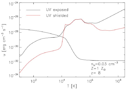
Figure 1: Radiative heating/cooling rates of UV exposed/shielded gas as a function of temperature. The black lines denote the radiative heating/cooling curves when gas are irradiated by the UV background radiation, while the red line denotes the collisional cooling curve where the UV is shielded. Except for the existence of the UV radiation, the other conditions are the same as $n_{\mathrm{H}}=0.03$ cm^-3, Z=1 Z_⊙, and $z=8$.

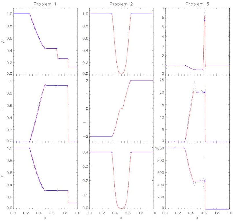
Figure 2: Three comparisons of the one-dimensional Riemann shock tube problem between analytic solution (red line) and the simulations (blue dots).

5 Astrophysical Processes

In addition to the basic hydrodynamic algorithms, we implement the following astrophysical processes in the EU$N$HA code: (1) non-adiabatic evolution of the gas particles through radiative cooling, (2) global reionization heating, (3) star formation, and (4) energy and metallicity feedbacks by supernova type II (SN_II) explosion.

5.1 Radiative Heating and Cooling

Using the CLOUDY package (version 10.10; Ferland et al. 1998), we calculated the heating and cooling rates and tabulated them in four terms of the gas density ($\rho$), temperature ($T$), metallicity ($Z$), and redshift ($z$) combining the effects of Compton heating/cooling, inverse Compton cooling, atomic/molecular cooling, and background UV heating. We assume that the whole simulation box is instantaneously full of the UV photons emitted by massive Pop-III stars at $z_{re}=8.9$ (Haardt & Madau 1996). With this step-function like global reionization process, we calculate the collisional ionization before $z_{re}$ and the photoionization after $z_{re}$. Also to reflect the self-shielding effect when a dense gas cloud is optically thick against the background UV radiation, we adopt the critical hydrogen number density, $n^{s}_{\mathrm{H}}$, above which the UV background radiation is effectively blocked. In this study, we set $n^{s}_{\rm H}=0.014~{}\mathrm{cm}^{-3}$ following Tajiri & Umemura (1998) and Sawala et al. (2010). Figure 1 shows the heating/cooling rates of UV exposed/shielded gas. The UV-irradiated gas is gradually heated up to the equilibrium temperature $T_{\mathrm{eq}}$, at which the UV heating and molecular cooling are balanced with each other. However, the UV-shielded gas may continuously be cooled down.

5.2 Star Formation

During the simulation run, we transform a gas particle into a star particle when the gas particle satisfies all the following star formation criteria (Katz, 1992): (1) $n_{\mathrm{H}}>0.1~{}\mathrm{cm}^{-3}$, (2) cosmic virialization condition or $\rho_{g}>57.5\left<\rho_{\mathrm{g}}\right>$, where $\left<\rho_{\mathrm{g}}\right>$ is the global value of gas density $\rho_{\mathrm{g}}$ at the redshift, (3) $T<10^{4}$ K, and (4) $\nabla\cdot{\mathbf{v}}<0$ for the convergent flow.

The star formation rate is calculated according to the Schmidt law as

$$\frac{d\rho_{*}}{dt}=c_{*}\frac{\rho_{g}}{t_{\mathrm{dyn}}},$$ (30)

where $\rho_{*}$ is the density of newly born stars, $c_{*}$ is the characteristic star formation efficiency, and $t_{\mathrm{dyn}}$ is the dynamical timescale of the gas particle. In this study, we adopt the standard star formation efficiency ($c_{*}=0.0333$) as adopted by Abadi et al. (2003). The dynamical time scale of a gas particle is defined as

$$t_{\rm dyn}\equiv\left({{G\rho_{g}}}\right)^{-1/2}.$$ (31)

The probability of a gas particle to be a star particle is given by the exponential law as

$$P=1-\exp\left(-c_{*}\frac{dt}{t_{\mathrm{dyn}}}\right).$$ (32)

and for each time step we determine whether a gas particle satisfying all the star formation criteria would be converted to a star particle by generating a random number and applying the probability function in equation (32). As the mass resolution of cosmological simulations may not reach individual stellar mass, each star particle actually represents a star cluster whose individual stars follow the stellar mass function of Kroupa (2001) with the mass range of 0.1–100 M_⊙.

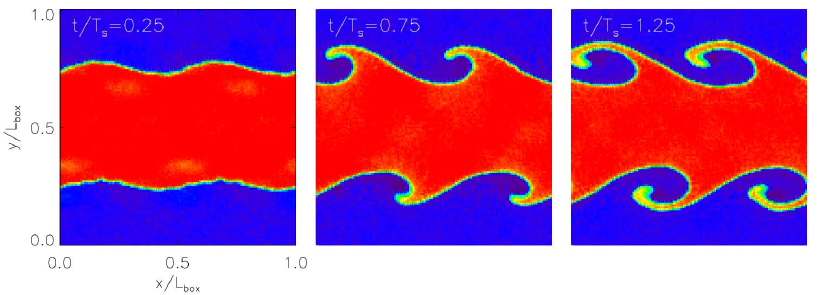
Figure 3: Density maps of flows at $t=0.25$, 0.75, and $1.25~{}T_{s}$. The red color denotes high density region moving right, while the blue color denote low density region moving to the left. The vortex-like structures are getting prominent with time.

5.3 Supernova Feedback

Stars follow different evolutionary tracks for different stellar mass and metallicity. As the SN_II explosion releases a large amount of energy and metals, and affects the phase state of the interstellar medium, it would be important to include the SN_II explosions in a high resolution cosmological simulation. For each star particle, we calculate the number of massive stars which may eventually end up as SN_II explosions using the stellar evolutionary model of Hurly, Pols & Tout (2000). Similar to the star formation recipe, we consider the SN_II feedback using the probability distribution (Okamoto, Nemmen, & Bower, 2008) as

$$P_{\mathrm{SN}}(Z)=\frac{\int_{t}^{t+dt}r_{\mathrm{SN}}(t^{\prime},Z)dt^{\prime}}{\int_{t}^{t_{\mathrm{max}(Z)}}r_{\mathrm{SN}}(t^{\prime},Z)dt^{\prime}},$$ (33)

where $r_{\mathrm{SN}}(t,Z)$ is the SN_II explosion rate as a function of time and the metallicity ($Z$). $t_{\mathrm{max}}(Z)$ is the maximum life time of the massive stars. Typically, $t_{\rm max}(Z)$ is known to be less than ten million years.

We assume that the supernova explosion affects nearby gas particles through heating and metal enrichment. For this purpose the SPH-like scheme is adopted to distribute the energy and metals to the nearby gas particles. The total amount of energy released by a supernova explosion is fixed to $10^{51}$ erg.

However the cooling time scale of the shock-heated gas is usually less than the hydro subtime step. Then, even though there is a temperature balance between radiative cooling and background heating, the simulated gas would not attain the equilibrium. This is the time-resolution problem in the gas cooling. To overcome this resolution problem, we precalculated the temperature evolutions with much finer time steps as

$$T(t+dt)=T(t)+\int_{0}^{dt}\left(n_{H}^{2}\Gamma(\rho,T,Z)+\Lambda(\rho,T)\right)dt_{T},$$ (34)

where $\Gamma$ is the cooling rate, $\Lambda$ is the heating rate, and the temperature time step size is numerically set as $dt_{T}=dt/100$. At every global time step, we tabulate the temperature evolution as a function of the gas density, temperature, metallicity, and time interval ($dt$). The metal enrichment is measured based on the tables given in Woosley & Weaver (1995).

6 Code Tests

To test the SPH algorithms and the implemented astrophysical processes, we perform five test simulations which are the most prominent topics that have been studied : (1) one-dimensional Riemann problems, (2) Kelvin-Helmholtz instability, (3) three-dimensional blast shock wave, (4) star formation on the isolated galactic disk, and (5) global star formation history in the cosmological context. Since the first three tests are designed to verify the hydrodynamics, we turn off gravity and astrophysical processes. We assume static backgrounds except in the last case. In the last two tests, we include gravity and astrophysical processes. Cosmic expansion is included only in the last case.

6.1 One-Dimensional Riemann Problems

In this subsection, we consider three cases of the one-dimensional Riemann problem in various shock conditions: a weak shock (Problem 1), a strong rarefaction shock (Problem 2), and an extremely strong shock (Problem 3). We adopt the initial conditions given in Springel (2010) and briefly describe them below. Periodic boundary conditions are imposed with $0\leq x<1$. The initial conditions simulating a shock front are chosen in the form of discontinuity in density ($\rho$), pressure ($P$), and particle velocity ($v$). Here, the subscript $L$ denotes the region 1 ($x\leq 0.5$) and subscript $R$ is used for region 2 ($x>0.5$). For Problem 1, the initial conditions are $(\rho,P,v)=(1,1,0)_{L}$ and $(0.125,0.1,0)_{R}$ for Region 1 and 2, respectively. For Problem 2, we set $(1,0.4,-2)_{L}$ and $(1,0.4,2)_{R}$. And for Problem 3, we arrange $(1,1000,0)_{L}$ and $(1,0.01,0)_{R}$. We used $\gamma=1.4$ in these tests and the number of neighbors is fixed to 7.

We compare the SPH results with the analytical solutions of Sod (1978) at $t=0.05$ in Figure 2. The density, particle velocity, and pressure are shown for Problem 1 (left column), Problem 2 (middle), and Problem 3(right), respectively. In the weak and strong rarefaction shock model, the simulated profiles well match the analytic solutions. However, there are scatters at the contact discontinuity and the shock front is not sharp due to the smoothing features of the SPH. Also, in the extremely-strong shock model we observe that the simulated profiles of the density, velocity, and pressure show larger deviations from the analytic solutions between the rarefaction and the shock front. However, these features are also seen in the standard SPH simulation as shown in other papers.

6.2 Kelvin-Helmholtz Instability

Agertz et al. (2007) have argued that the standard SPH algorithm cannot correctly model contact discontinuities like the Kelvin-Helmholtz (KH) instability. There have been several attempts to properly handle the instability by modifying the SPH algorithms (Price, 2008; Wadsley et al., 2008; Read, et al., 2010). We examine the issue of contact discontinuities in the case of the shear flows.

The initial condition of the test is laid out to satisfy the periodic boundary conditions of the cubic box on a side length of $L_{\mathrm{box}}=0.001~{}\mathrm{Mpc}$, in which we distribute $128^{3}$ gas particles. We divide the simulation box into two regions, the central region (hereafter Region 1) of $\mid y/L_{\mathrm{box}}-0.5\mid<0.25$ and the outer region (Region 2). Region 1 has a density ratio of $\rho/\rho_{c}=2$, where $\rho_{c}=7.22\times 10^{7}~{}\mathrm{M}_{\odot}/\mathrm{kpc}^{3}$, an $x$-directional velocity of $v_{x}=0.5~{}V_{s}$, where $V_{s}=8.8~{}\mathrm{km/s}$. The outer region is set to have $\rho/\rho_{c}=1$ and $v_{x}=-0.5V_{s}$. Region 1 has a temperature 50000 K and the temperature of Region 2 is doubled to maintain pressure equilibrium at the contact discontinuity.

We perturb the equilibrium by adding a $y$-directional velocity $v_{y}$ as

$$v_{y}(X,Y) = \omega_{0}\sin(4\pi X)V_{s}$$ (35)

$$\times \left[e^{-{(Y-0.25)^{2}/2\sigma^{2}}}+e^{-{(Y-0.75)^{2}/2\sigma^{2}}}\right],$$

where $X\equiv x/L_{\mathrm{box}}$, $Y\equiv y/L_{\mathrm{box}}$, $\omega_{0}=0.1$, and $\sigma=0.05/\sqrt{2}$ following Springel (2010).

Figure 3 shows the temporal evolution of density field at three different epochs, $t=0.25$, $0.75$ and $1.25~{}T_{s}$, where $T_{s}=55.52$  Myr. As the vertical perturbation grows, the horizontal ($x$-direction) shear flows generate vortex structures around the contact plane. The expected whirlpool-like structure gets prominent with time. It is well known that the standard SPH algorithm has a problem in reproducing the shear vortex of the KH instability (McNally et al., 2012; Hubber et al., 2013; Read, et al., 2010). Many authors have suggested that a modification to the SPH algorithms would be required to produce KH vortex, for example, the artificial thermal conductivity (Price, 2008; Agertz et al., 2007), a suitable smoothing kernel (Valcke et al., 2010), the Gudunov-SPH formalism (Cha et al., 2010), a diffusion term (Wadsley et al., 2008), the pressure-entropy formulation (Hopkins, 2013), or the moving mesh (Heß & Springel, 2010). Our findings are similar to that of Price (2008) who argued that particle noise at the discontinuity may suppress the growth of instability. The typical method to identify neighbor particles is to use the predict-correct algorithm, which is sometimes erroneous leading to noise. However, it is too far-fetched to tell whether our implementation of the neighbor searching method would solve the KH instability problem. The only thing we can say is that our neighbor finding may be one of the “partial” solutions to the KH instability problem. Further tests would be required to quantitatively compare EU$N$HA results with others.

6.3 Three-Dimensional Blast Wave

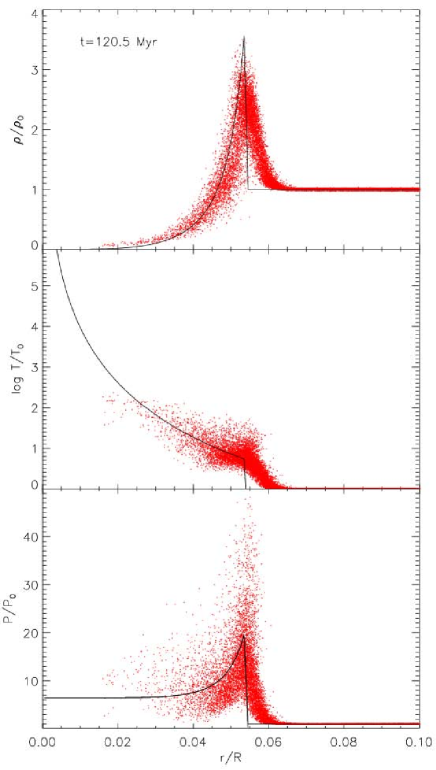
Figure 4: Density (top), temperature (middle) and pressure (bottom panel) profiles of three-dimensional Sedov blast wave. Here, $r$ is the distance from the central particle. The red dots denote the simulation results and the black line shows the semi-analytic solution of Sedov (1959). The $x$-axis is scaled to the box size and the y-axis is normalized to the initial density, temperature and pressure of the test simulation.

We also investigated the three-dimensional Sedov blast wave test. A nearly homogeneous glass-like distribution of $256^{3}$ particles is created in the 100 kpc simulation box with total particle mass $7.22\times 10^{7}$M_⊙. The temperature of a gas particle is uniformly set to 10 K. We assign a huge temperature $T=10^{6}$ K to the particle located at the center of the box to simulate the supernova explosion. This generates a shock wave, which propagates outwards and sweeps away the surrounding cool and less-dense gas.

Figure 4 shows the comparison of density, temperature, and pressure profiles around the ground zero of explosion between the simulation (points) and semi-analytic solution (line; Sedov 1959) at $t=120.5$ Myr. Good agreement is seen both in the location of the shock front and the maximum density, with a substantial scatter around the analytic solution. The simulated upstream has a scatter of density with a finite slope because of the finite smoothing scale of the SPH and the anisotropic initial particle distribution. The regular lattice point of initial particle positions was adopted by Springel & Hernquist (2002) and Merlin et al. (2010) while a new setup is adopted to reduce anisotropic and inhomogeneous distribution in the shock propagation (Rosswog & Price, 2007).

6.4 Isolated Galaxy

Figure 5: Density-weighted temperature map of gas disk. The dense spiral arms are cooled down more efficiently than the less-dense regions through the more efficient radiative cooling. Red clumps along the spiral structures represent the shock-heated gas by the SN_II explosions among the recently-forming massive stars.

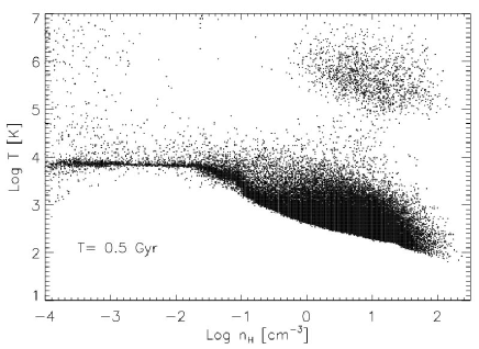
Figure 6: $n_{\mathrm{H}}$–$T$ diagram of gas particles at $T=0.5$ Gyr. All gas particles are irradiated by UV backgrounds because we assume that there is no self-shielding in this test. Thus, most of simulated particles are distributed along the equilibrium temperature line. The scatters around the equilibrium temperature is mainly due to adiabatic expansion and contraction. Points in the upper-right corner are the shock-heated gas particles due to the nearby SN_II explosions. After a transient period, their density will drop due to expansion and points will move to the upper-left corner of the box.

Now, we investigate the stability of galaxy disk and the star formation rate on the disk plane using the isolated galaxy model. The initial conditions of a multi-component galaxy were generated according to the isolated Milky-Way model proposed by Hernquist (1993). An exponential gas disk is arranged with a characteristic mass $M_{g}=4.125\times 10^{9}\mathrm{M}_{\odot}$, disk scale height $z=0.3$ kpc, and disk scale length of $h=3.33$ kpc. An exponential stellar disk is built with $M_{s}=3.715\times 10^{10}~{}\mathrm{M}_{\odot}$, $z=0.3$ kpc, and $h=3.33$ kpc. The bulge component follows Hernquist profile with $M_{b}=1.375\times 10^{10}~{}\mathrm{M}_{\odot}$ and scale length of $a=0.8$ kpc. The halo component follows the Hernquist model with parameters $M_{h}=2.2\times 10^{11}~{}\mathrm{M}_{\odot}$ and $a=10$ kpc. The three-dimensional locations and velocities of particles are calculated by ZENO software package developed by Joshua E. Barnes. The gas and stellar disks are composed of 983,040 particles with particle mass of $M_{p}=4.196\times 10^{4}~{}\mathrm{M}_{\odot}$ while the bulge and halo structures are treated as fixed external potentials. We set the initial temperature of gas particles to be $10^{4}$ K.

Figure 5 shows the density-weighted temperature map of the gas disk at $t=0.5$ Gyr. Gas particles of $T<10^{4}$ K are distributed along spiral structures, where density is so high that the gas is able to cool down to lower temperature through efficient radiative cooling. Density-temperature distribution of gas particles under radiative heating and cooling process are shown in Figure 6. We can see that gas particles in the low density regions keep the initial temperature of $T\sim 10^{4}$ K, while the gas particles in the higher density regions may cool down to lower temperature toward the equilibrium state. Stars form in the high-density and low-temperature regions along the spirals. Tens of million years after star formation, the SN_II explosions of the massive stars redistribute thermal energy into the surrounding interstellar medium. The red clumps in Figure 5 represent the highly heated gas particles near the supernova explosion sites.

Finally, we compare the simulated star formation rate with the observed value in Figure 7. The projected star formation rates on the gas disk $\Sigma_{\mathrm{SFR}}$ for a given column density $\Sigma_{\mathrm{gas}}$ well reproduce the observed Schmidt-Kennicutt relation (Kennicutt, 1998).

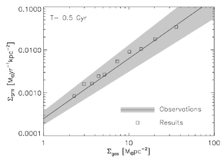
Figure 7: Projected star formation rate $\Sigma_{\mathrm{SFR}}$ versus the column density $\Sigma_{\mathrm{gas}}$ on the simulated disk at 0.5 Gyr. The solid line enclosed by the gray-shaded region represents the observed Kennicutt relation with errors (Kennicutt 1998), and squares are the simulation results.

6.5 Cosmological Model

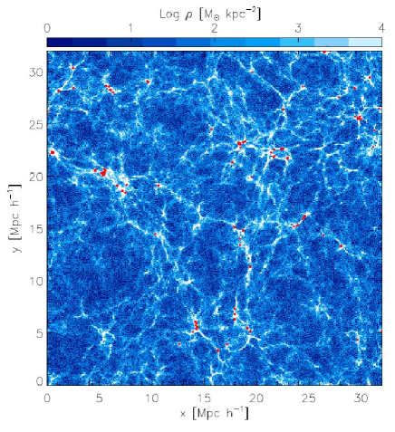
Figure 8: Projected density map of gas particles in a $z$-directional slab with a width equal to three times of the mean particle separation at the epoch of $z=6$. Red dots represent newly formed star particles, and they are located in cluster regions.

Figure 9: $n_{\mathrm{H}}$–$T$ diagram of gas particles at $z=6$. The solid line marks the UV-background shielding density of $n_{\mathrm{H}}=0.014~{}\mathrm{cm}^{-3}$.

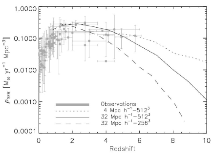
Figure 10: Comparison of star formation histories of the universe between the simulation results (three different lines) and the observations (shaded symbols with error bars). The simulation results are differed by resolutions, different box size and particle number. The observed data is compiled by Hopkins & Beacom (2006).

Now, we turn our attention to the application of EU$N$HA to cosmological star formation. We solve the equation of motion of the gas and dark matter particles in a cubic simulation box of a side length $L_{\rm box}=32~{}h^{-1}{\rm Mpc}$. The total number of gas and dark matter particles is $512^{3}$. The cosmological model adopted in the simulation is the WMAP-5 year cosmology with parameters of $\Omega_{m}=0.26$, $\Omega_{\Lambda}=0.74$, $\Omega_{b}=0.044$, $\sigma_{8}=0.76$, $n_{s}=0.96$, and $h=72~{}\mathrm{km~{}s^{-1}~{}Mpc^{-1}}$. The simulation starts with glass-like pre-initial condition, which has a virtually null net gravitational force. To perturb pre-initial particle distribution, we applied the second-order linear perturbation method described in Jenkins (2010). The initial power spectra for baryonic and dark matter at redshift $z=150$ are calculated by the CAMB package (http://camb.info/sources). The initial background temperature of gas is calculated using the RecFast package (Seager, Sasselov, & Scott, 1999). In generating initial conditions, the density fluctuations of the gas particles may create temperature fluctuations. We determine the temperature fluctuation for each gas particle using the adiabatic model as

$$\Delta\ln~{}T=(\gamma-1)\Delta\ln\rho.$$ (36)

Figure 8 is an example of the gas density at $z=6$. The distribution of gas particles by and large follow those of dark matter particles such as clusters, filamentary structures, and cosmic voids. After the predefined cosmic reionization epoch at $z_{re}=8.9$, most of gas particles in low density regions of $n_{\mathrm{H}}<0.014~{}\mathrm{cm}^{-3}$ are heated up to $T_{g}\sim 10^{4}$ K, thus the distribution of the gas particles is more diffuse than dark matter particles. Meanwhile, gas particles located in high density regions ($n_{\mathrm{H}}>0.014~{}\mathrm{cm}^{-3}$), which are optically thick to the cosmic UV background, may cool down to lower temperature and, thus, settle down to the inner region of dark matter halos. The detailed density-temperature relation of gas particles are shown in Figure 9. Due to the gas inflow to the halo center, typically halo regions have $\nabla\cdot\mathbf{v}<0$. And as the inner regions of the halo have a high hydrogen density and low temperature, gas particles are able to cool and finally form stars therein. The red dots in Figure 8 represent the newly generated stars in clustered regions.

The observed global star formation rate ($\rho_{\mathrm{SFR}}$) of the Universe is known to be a function of redshift with a peak located among $z=2$–3. In Figure 10, we compare the star formation history of simulations (lines) with observations (symbols, Hopkins & Beacom 2006). The overall star formation history agrees with each other.

However, there are differences in the gradient of star formation rate ($\dot{\rho}_{\mathrm{SFR}}$) between three different simulations, and it is because of the different resolution. Choi & Nagamine (2012) reported that the lower mass galaxies are preferred sites for star formation in the higher redshift, thus slope of $\rho_{\mathrm{SFR}}(z)$ for the finer resolution is shallower than others. Among cosmological simulations, the highest resolution simulation with $L_{\rm box}=4~{}h^{-1}{\rm Mpc}$ and $512^{3}$ particles show the lowest $\dot{\rho}_{\mathrm{SFR}}$ but highest $\rho_{\mathrm{SFR}}$.

7 Summary and Conclusion

We have developed a new cosmological hydrodynamic simulation code (EU$N$HA) by combining the pre-existing $N$-body code of GOTPM (Dubinski et al., 2004) with the standard smoothed particle hydrodynamics (SPH). This code fully exploits the advantage of the Oct-Sibling Tree (OST) of the GOTPM to identify the $N$ nearest neighbors.

For astrophysical evolution of gas particles, we also implemented the processes of (1) non-adiabatic evolution of the gas particles through radiative heating/cooling, (2) global reionization, (3) star formation, and (4) energy and metallicity feedbacks by supernova type II explosion. To demonstrate our new implementations of the SPH and the astrophysical processes, we made five test simulations: (1) one-dimensional Riemann problems, (2) Kelvin-Helmholtz instability, (3) three-dimensional blast shock wave, (4) star formation on the isolated galactic disk, and (5) global star formation history in the cosmological context.

It is interesting to see the growth of the shear vortex in the Kelvin-Helmholtz instability test because the only difference in EU$N$HA from other standard SPH methods is the neighbor searching. Even though it is premature to conclude in this simple test, we may get a hint from Price (2008), who showed that the particle noise on the shear contact plane may be one of the possible causes to the suppressed KH instabilities. Our improved neighbor searching method may reduce this kind of neighboring noise in the predict-correct method. The SPH measures hydrodynamic quantities of a gas particle using nearby interacting neighbors contained by a finite smoothing length. Therefore, the gas density, pressure, and corresponding acceleration may change for different smoothing lengths. It means that during a simulation run a sudden change in the number of interacting neighbors may also have a sudden impact on the gas motion. Then, small perturbations may be buried in the numerical noise and may be suppressed from developing on the contact layer. However, it is too hasty to jump to the conclusion with this simple result because some authors already showed that with different initial conditions the KH vortex can grow even in the standard-SPH test (Hopkins, 2013) but with much less surface mixing than shown in other grid-based tests. Also Price (2008) showed that a standard SPH test may yield a small KH vortex by adjusting the test parameters. So, it is unclear whether our implementation of the advanced neighbor searching solves the KH instability problem in the Lagrangian code. Our tentative conclusion is that our code may develope the KH vortex but the surface mixing on the contact plane seems to be not so strong as other improved versions of the SPH or Eulerian codes. More rigorous tests will be necessary to draw any conclusion on this issue.

The EU$N$HA code is originally intended to serve as the basis for the further development of the cosmological hydrodynamic simulation code. Most hydrodynamic routines are built for fast and efficient communication between the parallel ranks, and the SPH functions is carefully organized to be isolated (or modularized) for flexibility in case of future updates. Therefore, we may be able to easily exchange the SPH routines with those of another type of the particle-based hydrodynamic algorithms.