Stabilizing Sparse Cox Model using Clinical Structures in Electronic Medical Records

Abstract

Stability in clinical prediction models is crucial for transferability between studies, yet has received little attention. The problem is paramount in high-dimensional data which invites sparse models with feature selection capability. We introduce an effective method to stabilize sparse Cox model of time-to-events using clinical structures inherent in Electronic Medical Records (EMR). Model estimation is stabilized using a feature graph derived from two types of EMR structures: temporal structure of disease and intervention recurrences, and hierarchical structure of medical knowledge and practices. We demonstrate the efficacy of the method in predicting time-to-readmission of heart failure patients. On two stability measures – the Jaccard index and the Consistency index – the use of clinical structures significantly increased feature stability without hurting discriminative power. Our model reported a competitive AUC of 0.64 (95% CIs: [0.58,0.69]) for 6 months prediction.

1 Introduction

Heart failure is a serious illness which demands frequent hospitalization. It is estimated that 50% of heart failure patients are readmitted within 6 months after their discharge [4]. A significant amount of these readmissions can be predicted and prevented. Existing readmission prediction models use diverse subsets of clinical variables from prior hypotheses or medical literature [9], making it hard to reach a consensus of what are predictive and what are not. With the emergence of electronic medical records (EMR), it is now possible to obtain data on all aspects of patient care over time. A typical EMR database contains full details about demographics, history of hospital visits, diagnosis, procedures, physiological measurements, bio-markers and interventions that are recorded over time [5]. Such high-dimensional data is comprehensive but calls for robust feature selection when deriving prediction models. Unfortunately, automatic feature selection, particularly in clinical data, has been known to cause instability in features against data sampling, and thus limiting the reproducibility of the model [1]. Improving stability of model estimation is crucial, but it has received little attention.

We investigate time-to-readmission due to heart failure using a sparsity-inducing Cox model [10] on high-dimensional EMR data. Our objective is to improve the stability of this sparse model by exploiting clinical structures inherent in the EMR data. Specifically, we make use of (i) temporal relations in diagnosis, prognosis and intervening events, and (ii) hierarchical structures of disease family through semantics in ICD-10 tree and procedure pool (ACHI) . These structures are encoded into a feature graph with its edges representing the relation between features. The application of feature graph ensures sharing of statistical strength among correlated features, thereby promoting stability. The proposed stabilized sparse Cox model is trained and validated using retrospective data from a local hospital in Australia. Model stability is validated using measures of Jaccard index [8] and Consistency index [6]. We demonstrate that by exploiting inherent clinical structures in EMR, the stability of our regularized Cox model is improved without loss in performance.

2 Method

We describe a method to utilize inherent structures in data to stabilize sparse Cox model derived from EMR databases. To start with, we employed the one-sided convolutional filter bank introduced in [11] to extract a large pool of features from EMR databases. The filter bank summarizes event statistics over multiple time periods and granularities.

2.1 Sparse Cox Model

We use Cox regression to model risk of readmission due to heart failure (hazard function) at a future instant, based on data from EMR. Unlike logistic regression where each patient is assigned a nominal label, Cox regression models the readmission time directly [12]. The proportional hazards assumption in Cox regression assumes a constant relationship between readmission time and EMR-derived explanatory variables. Let $\mathcal{D}=\left\{\boldsymbol{x}_{\ell},y_{\ell}\right\}_{\ell=1}^{n}$ be the training dataset, ordered on increasing $y_{\ell}$, where $\boldsymbol{x}_{\ell}\in\mathbb{R}^{p}$ denotes the feature vector for $\ell^{th}$ index admission and $y_{\ell}$ is the time to next unplanned readmission. When a patient withdraws from the hospital or does not encounter readmission in our data during the follow-up period, the observation is treated as right censored. Let $q$ observations be uncensored and $R(t_{\ell})$ be the remaining events at readmission time $t_{\ell}$.

Since the data $\mathcal{D}$ is high dimensional (possibly $p\gg n$), we apply lasso regularization for sparsity induction [10]. The feature weights $\boldsymbol{w}\in\mathbb{R}^{p}$ are estimated by maximizing the $\ell_{1}$-penalized partial likelihood:

$$\mathcal{L}_{1}^{reg}=\frac{1}{n}\mathcal{L}\left(\boldsymbol{w};\mathcal{D}\right)-\alpha\|\boldsymbol{w}\|_{1}$$ (1)

where $\|\boldsymbol{w}\|_{1}=\sum_{i}\left|w_{i}\right|$, $\alpha>0$ is the regularizing constant, and $\mathcal{L}\left(\mathbf{w};\mathcal{D}\right)$ is the log partial likelihood [3] computed as:

$$\overset{{}_{q}}{\underset{{}_{\ell=1}}{\sum}}\left\{\boldsymbol{w}^{\top}\boldsymbol{x}_{\ell}-\log\left[\underset{\jmath\in R(t_{\ell})}{\sum}\exp\left(\boldsymbol{w}^{\top}\boldsymbol{x}_{\jmath}\right)\right]\right\}$$

The lasso induces sparsity by driving the weights of weak features towards zero. However, sparsity induction is known to cause instability in feature selection [13]. Instability occurs because lasso randomly chooses one in two highly correlated features. Each training run with slightly different data could result in a different feature from the correlated pair. The nature of EMR data further aggravates this problem. The EMR data is, by design, highly correlated and redundant. Also, features in the EMR data maybe weakly predictive for some task, thereby limiting the probability that they are selected. These sum up to lack of reproducibility between model updates or external validations, hindering the method credibility and adoption by clinicians.

2.2 Stabilizing with Clinical Structures

A natural solution to the instability problem is to ensure that correlated features are assigned with similar weights. We exploited two clinical structures inherent in the EMR data for this purpose. The first is temporal structure of diagnosis, hospital interaction and intervening events recorded over time. The second is code structure based on hierarchies in medical knowledge and practices such as International Classification of Disease, $10^{th}$ revision (ICD-10) and procedure codes. Two codes are considered to be correlated if they share the same prefix. Using the temporal structure of events, and the hierarchical structure of code trees, we built an undirected graph with features as nodes and edges representing the relation between features. Let $\mathbf{A}\in\mathbb{R}^{p\times p}$ be the incidence matrix of the feature graph with $A_{ij}=1$ if features $i$ and $j$ share a temporal or code relation, and $A_{ij}=0$ otherwise. We introduced a graph regularizing term to Eq. (1):

$$\mathcal{L}_{2}^{reg}=\mathcal{L}_{1}^{reg}-\frac{1}{2}\beta\underset{{}_{ij}}{\sum}A_{ij}(w_{i}-w_{j})^{2}$$ (2)

where the term $\underset{{}_{ij}}{\sum}A_{ij}(w_{i}-w_{j})^{2}$ ensures similar weights for correlated features, and $\beta>0$ is the correlation coefficient.

The graph regularization term $\sum_{ij}A_{ij}(w_{i}-w_{j})^{2}$ can be expressed as:$\underset{{}_{i}}{\sum}\left(\underset{{}_{j}}{\sum}A_{ij}\right)w_{i}^{2}-\underset{{}_{ij}}{\sum}A_{ij}w_{i}w_{j}$. Let $\mathbf{L}$ denote the Laplacian of feature graph $\mathbf{A}$, where $L_{ii}=\Sigma_{j}A_{ij}$ and $L_{ij}=-A_{ij}$ [2], the graph regularization term now becomes $\boldsymbol{w}^{\top}\mathbf{L}\boldsymbol{w}$. Eq. (2) can be rewritten as:

$$\mathcal{L}_{2}^{reg}=\frac{1}{n}\mathcal{L}\left(\boldsymbol{w};\mathcal{D}\right)-\alpha||\boldsymbol{w}||_{1}-\frac{1}{2}\beta\,\boldsymbol{w}^{\top}\mathbf{L}\boldsymbol{w}$$ (3)

The gradient of Eq.(3) becomes:

$$\frac{\partial\mathcal{L}_{2}^{reg}}{\partial\boldsymbol{w}} = \overset{{}_{q}}{\underset{{}_{\ell=1}}{\sum}}\left\{\boldsymbol{x}_{(\ell)}-\frac{\underset{\jmath\in R(t_{\ell})}{\sum}\boldsymbol{x}_{\jmath}\exp(\boldsymbol{w}^{\top}\boldsymbol{x}_{\jmath})}{\underset{\jmath\in R(t_{\ell})}{\sum}\exp(\boldsymbol{w}^{\top}\boldsymbol{x}_{\jmath})}\right\}$$ (4)

$$\quad\quad-\alpha\,\mbox{sign}(\boldsymbol{w})-\beta\boldsymbol{w}^{\top}\mathbf{L}$$

2.3 Measuring Model Stability

We used the Jaccard index [8] and the Consistency index [6] to measure stability of feature selection process. To simulate data variations due to sampling, we created $B$ data bootstraps of original size $n$. For each bootstrap, a model was trained and a subset of top $k$ features was selected. Features were ranked according to their importance, which is product of feature weight and standard deviation. Finally, we obtained a list of feature subsets $S=\left\{S_{1},S_{2},...,S_{B}\right\}$ where $\left|S_{b}\right|=k$.

The Jaccard index measures similarity as a fraction between cardinalities of intersection and union of feature subsets. Given two feature sets $S_{a}$ and $S_{b}$, the pairwise Jaccard index reads:

$$J_{C}(S_{a},S_{b}) = \frac{\left|S_{a}\cap S_{b}\right|}{\left|S_{a}\cup S_{b}\right|}$$ (5)

The Consistency index corrects the overlapping due to chance. Considering a pair of subsets $S_{i}$ and $S_{j}$, the pairwise Consistency index $I_{C}$ is defined as:

$$I_{C}(S_{a},S_{b})=\frac{rd-k^{2}}{k(d-k)}$$ (6)

in which $\left|S_{a}\cap S_{b}\right|=r$ and $d$ is the number of features. The stability for the set $S=\left\{S_{1},S_{2},...,S_{B}\right\}$ is calculated as average across all pairwise $J_{C}(S_{a},S_{b})$ and $I_{C}(S_{a},S_{b})$. Jaccard index is bounded in $\left[0,1\right]$ while Consistency index is bounded in $\left[-1,+1\right]$.

3 Results

We trained our model on 1,088 patients (1,405 index admissions) discharged from Barwon Health (a regional hospital in Australia) from Jan 2007 to Sept 2010. The model was validated on another cohort of 317 patients (369 index admissions) discharged from Oct 2010 to Dec 2011. From a total of 3,338 features, our model selected 94 features that are highly predictive of heart failure readmissions. The top predictors are listed in Table 1.

The discrimination of the model with respect to the area under the ROC curve (AUC) was investigated for various values of the hyperparameters $\alpha$ and $\beta$ (Fig. 3a). The AUC depends more on the lasso hyperparameter $\alpha$, which controls the number of features being selected. The best AUC for our model was 0.64 for $\alpha=.004$ and $\beta=.03$. Next, we investigated the role of the structure hyperparameter $\beta$ on feature stability against data resampling. For a fixed value of lasso regularization $\alpha=.004$, increase in $\beta$ resulted in increased stability of the top 90 features, confirmed by both Consistency index and Jaccard index (see Figs. 3b and c). Hence $\alpha$ affects model AUC, while $\beta$ affects feature stability.

Finally, the stability of feature subsets selected by the unregularized model and the regularized model with $\alpha=.004$ and $\beta=.03$ were compared for each bootstrap. Our proposed model regularized by clinical structures was found to be more robust to training data variations for all subset sizes when measured using both indices (Figs. 1 and 2).

Table 1: The top predictors for heart failure readmission identified by our proposed model.

Top Predictors	Importance
Male	100.0
Age > 90	86.3
Rare diagnosis in past 3 months	63.8
Past respiratory infection	55.0
Disease history in past 6-12 months	44.9
Pain in throat and chest	41.0
Chronic kidney disease	31.7
Abnormalities of heart beat	29.3
Disorders of kidney and ureter	25.2
Emerg. admits in past 1-2 years	48.1
Admissions in past 2-4 years	45.7
Emerg. admits in past 3 months	39.0
Emerg-to-ward in 0-3 months	35.3
Valvular disease past 3 months	28.8

Figure 1: Consistency index.

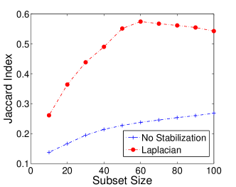
Figure 2: Jaccard index.

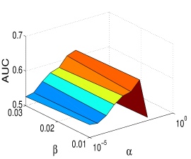
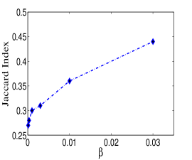
(a)	(b)	(c)

Figure 3: Effect of hyperparameters on (a) discrimination measured in AUC and (b,c) stability at 90 feature subsets.

4 Discussion

Feature stability facilitates reproducibility between model updates and generalization across medical studies. In this paper, we utilize the temporal and code structures inherent in EMR data to stabilize a sparse Cox model for heart failure readmissions. Though heart failure patients diagnosed with other comorbidities are more prone to rehospitalization [7], our model focuses on patients diagnosed solely with heart failure. When compared with similar studies, the model AUC is competitive and the top predictors including male gender, age, history of prior hospitalizations, presence of kidney disorders were found to be common [9]. Encoding clinical structures into feature graphs promotes group level selection and rare-but-important features. This resulted in our model selecting past rare diagnosis as an important predictor. On two stability measures, the proposed method has demonstrated to largely improved stability. Also, our proposed model is derived entirely from commonly available data in medical databases. All these factors suggest that our model could be easily integrated into the clinical pathway to serve as a fast and inexpensive screening tool in selecting features and patients for further investigation. Future work includes applying the same technique for a variety of cohorts and investigating other latent structures in EMR to enhance feature stability.

References

- [1] P. C. Austin and J. V. Tu. Automated variable selection methods for logistic regression produced unstable models for predicting acute myocardial infarction mortality. Journal of clinical epidemiology, 57(11):1138–1146, 2004.
- [2] F. R. Chung. Spectral graph theory, volume 92. American Mathematical Soc., 1997.
- [3] D. R. Cox. Partial likelihood. Biometrika, 62(2):269–276, 1975.
- [4] A. S. Desai and L. W. Stevenson. Rehospitalization for heart failure predict or prevent? Circulation, 126(4):501–506, 2012.
- [5] P. B. Jensen, L. J. Jensen, and S. Brunak. Mining electronic health records: towards better research applications and clinical care. Nature Reviews Genetics, 13(6):395–405, 2012.
- [6] L. I. Kuncheva. A stability index for feature selection. In Artificial Intelligence and Applications, pages 421–427, 2007.
- [7] R. Perkins, A. Rahman, I. Bucaloiu, E. Norfolk, W. Difilippo, J. Hartle, and H. Kirchner. Readmission after hospitalization for heart failure among patients with chronic kidney disease: a prediction model. Clinical nephrology, 2013.
- [8] R. Real and J. M. Vargas. The probabilistic basis of jaccard’s index of similarity. Systematic biology, 45(3):380–385, 1996.
- [9] J. S. Ross, G. K. Mulvey, B. Stauffer, V. Patlolla, S. M. Bernheim, P. S. Keenan, and H. M. Krumholz. Statistical models and patient predictors of readmission for heart failure: A systematic review. Archives of Internal Medicine, 168(13):1371–1386, 2008.
- [10] R. Tibshirani et al. The lasso method for variable selection in the cox model. Statistics in medicine, 16(4):385–395, 1997.
- [11] T. Tran, D. Q. Phung, W. Luo, R. Harvey, M. Berk, and S. Venkatesh. An integrated framework for suicide risk prediction. In KDD, pages 1410–1418, 2013.
- [12] B. Vinzamuri and C. Reddy. Cox regression with correlation based regularization for electronic health records. In Data Mining (ICDM), 2013 IEEE 13th International Conference on, pages 757–766, Dec 2013.
- [13] H. Xu, C. Caramanis, and S. Mannor. Sparse algorithms are not stable: A no-free-lunch theorem. Pattern Analysis and Machine Intelligence, IEEE Transactions on, 34(1):187–193, 2012.