Stabilized Sparse Ordinal Regression for Medical Risk Stratification

Abstract

The recent wide adoption of Electronic Medical Records (EMR) presents great opportunities and challenges for data mining. The EMR data is largely temporal, often noisy, irregular and high dimensional. This paper constructs a novel ordinal regression framework for predicting medical risk stratification from EMR. First, a conceptual view of EMR as a temporal image is constructed to extract a diverse set of features. Second, ordinal modeling is applied for predicting cumulative or progressive risk. The challenges are building a transparent predictive model that works with a large number of weakly predictive features, and at the same time, is stable against resampling variations. Our solution employs sparsity methods that are stabilized through domain-specific feature interaction networks. We introduces two indices that measure the model stability against data resampling. Feature networks are used to generate two multivariate Gaussian priors with sparse precision matrices (the Laplacian and Random Walk). We apply the framework on a large short-term suicide risk prediction problem and demonstrate that our methods outperform clinicians to a large-margin, discover suicide risk factors that conform with mental health knowledge, and produce models with enhanced stability.

1 Introduction

The recent wide adoption of Electronic Medical Records (EMRs) offers great opportunities for mining useful patterns that support clinical research and decision making [27]. The EMR contains rich information about a patient, including demographics, history of hospital visits, diagnoses, physiological measurements, bio-markers and interventions. We consider the problem of predicting risk stratification using EMR data. By ‘risk’ we mean unwanted outcomes such as readmissions, length of hospitalization, intoxication and mortality. For clinical use, the outcomes are often stratified into ordered levels such as “low”, “moderate” and “high” risk. We aim at constructing a scalable automated framework that takes entire historical medical records for each patient and predicts ordered risk within a window.

The challenges lie in effective and interpretable modeling of noisy, irregular, temporal and mixed modalities [37, 66]. An EMR can be considered as a mixture of static information and time-stamped events. Static information includes demographic variables and thus is generally moderate in dimensions. The events are, however, complex and high dimensional. For example, the current disease coding scheme ICD-10 has approximately $20,000$ entries, and the number adds up quickly if we consider multiple time scales and the combination with other event types (e.g., medications). Events are often packed into episodes of admissions and treatments, and thus are highly irregular.

The high dimensional data calls for sparse predictive models [61, 68]. Unfortunately, sparse models could be unstable against data variations. The instability can be measured as the probability that a feature is selected [41] or as the variance in model parameters. In EMR, features can be highly correlated, and thus sparse models often pick the strongest one seen in the data sample [67, 72]. Under data resampling, another feature may be chosen next time. Second, for some tasks, EMR-derived features could be weakly predictive, thus limiting the probability that they are selected. Unstable models are less useful in practice because they cannot generalize from one cohort to another, and thus undermining the research reproducibility and reducing the clinician adoption.

In this paper, we present a two-stage stabilized sparse ordinal framework that addresses these challenges [64]. The first stage extracts a large number of features from EMR. The extraction builds on a novel conceptual view in which a patient’s medical records forms a temporal image, from which filters over different time windows extract a diverse feature set. Multi-class ordinal classification is then formulated in two main ways—with and without class-specific parameters. For each set, risk is transparently modeled as either cumulative risk [40] or stagewise progression of risk [65, 63]. The ordinal classifiers are equipped a $\ell_{1}$-norm penalty which yields sparse solutions. The selection is stabilized through relational regularization, in which domain-specific feature interaction is used to promote smoothness among related parameters. Examples of interaction include the “sibling” relation between two diagnosis codes in the same disease branch, or the progression of a disease. To measure model stability, we introduce two stability indices, evaluated at any feature ranked list length, one accounts for the feature selection probability and the other computes the signal-to-noise ratio in the feature weights.

Our framework is demonstrated through a large cohort of ten of thousands of mental health patients who were under assessment for suicide risk. This problem devastates families and communities: One out of ten persons develop suicidal thoughts in their lifetime [45], and 0.3 percents attempt suicide in any given year [8]. In response, health services introduced mandatory suicide risk assessment for vulnerable populations [2]. These assessments form the basis of suicide risk stratification. But traditional suicide risk assessment lacks prediction accuracy [31, 54]. Providing more accurate solutions for suicide risk stratification will deliver immediate benefits. The challenges are that data is highly sparse; many risk factors are known, but they are weakly predictive.

The framework is evaluated against several criteria: predictive accuracy against clinicians, the degree to which discovered features conform with clinical knowledge, and model stability. In predicting risk, the framework outperforms the mental health professionals in a large margin. For moderate-risk prediction, machines improve the $F_{1}$-score by $25\%$. For the high-risk class, the improvement are as high as $200\%$. In terms of suicide detection, the machine detects $29-30$ cases, which are more than double the number detected by human ($14$ cases). The discovered features agree with most previously reported risk factors which came out of decades of extensive research. The results are significant as the framework relies entirely on data readily collected in hospitals, and the risk prediction is objective and transparent. We also demonstrate the efficacy of our feature stabilization methods vs no stabilization.

In short, this paper contains the following contributions:

• A generic and scalable risk stratification framework with three components: (i) A novel conceptual view of EMR as a temporal image so that a diverse set of features at different temporal scales can be extracted; (ii) Modeling of risk through ordinal classification, in particular the introduction of stagewise risk modeling in this context; (iii) Formulation of methods to stabilize predictive models, through appropriate relational regularization of the risk functional in ordinal classification.

• Two model stability indices over arbitrary feature rank list size, one is based on probability that a feature is selected, and the other on signal-to-noise ratio of the feature weights. A related contribution is a novel stability-based feature ranking criterion based on the signal-to-noise ratios.

• Comprehensive evaluation of methods in comparison with clinicians, demonstrating that machine learning methods outperform clinicians in risk stratification. It demonstrates the value of mining EMR data for an important problem. To the best our knowledge, this is the first study that formulates suicide risk prediction as a data mining task and leads to a solution being clinically adopted.

• The framework can be generalized to a variety of disease. Given mixed type data comprising demography, clinical history (emergency attendances, admissions and diagnostic coding), and risk assessment instruments (questions with ordinal ratings), our framework automatically extracts the most relevant features and builds stabilized risk prediction classifiers.

The paper is organized as follows. The next section reviews related work. Section 3 presents an overview of the framework. Section 4 describes EMR data representation and feature extraction. Ordinal classifiers are derived in the subsequent section, followed by the relational stabilization method in Section 6. Section 7 details implementation issues and results. Section 8 provides further discussion, followed by the conclusion.

2 Background

Risk stratification is important in medical practice and research [59]. There are two major prediction types: diagnosis (estimating the probability that a disease is present) and prognosis (predicting the outcomes given current diagnoses or intervention plan). These estimation and prediction influence clinical practices such as test ordering, treatment/discharge planning and resource allocation. In medical research, knowing the risk helps selecting cohorts for randomized trials and assessing risk aspects and confounding factors.

The established risk model construction strategy relies on small hand-picked subset of features from highly stratified cohorts [46, 59]. As a result, previous studies were fragmented where conclusion only holds under well-controlled conditions. Electronic Medical Record (EMR), on the other hand, suggests a data-centric and hypothesis-free approach from which data mining techniques can be utilized. It typically contain a diverse set of information types, including demographics, admissions and diagnoses, lab tests and treatments. Research into machine learning for EMRs is largely recent and fast growing [27]. However, automating the learning process is still limited. In our work, we generate, select and combine thousands of weak signals in an automated fashion.

Sparsity and Stability

The nature of such high-dimensional setting leads to sparse models, where only small subsets of strongly predictive signals are kept. Such sparsity leads to better interpretability and generalization; this is expected to play an important role in biomedical domains [68]. However, sparse models alone are not enough in practice. We need stable models, that is, models that do not change significantly with data sampling. Stable models are reproducible and generalizable from one cohort to another. However, sparsity and stability could be conflicting goals [67], especially when noise is present [17]. Most sparsity-inducing algorithms do not aim at producing stable models. For example, stepwise feature selection in logistic regression produces unstable models [3]. In the context of lasso, only one variable is chosen if two are highly correlated [72].

Model stability is related but distinct from prediction stability – the predictive power does not change due to small perturbation in training data [9]. It is quite possible that unstable models can still produce stable outputs. Stable models, on the other hand, lead to stable prediction under regular conditions often seen in practice. Model stability is a stronger requirement than recently studied feature selection stability issues [6, 33]. Stable feature selection algorithms produce similar feature subsets under data variation; whilst model stability also considers feature weights.

Several model stability indices have been introduced recently [23, 28, 29, 33, 57]. A popular strategy is to consider similarity between any feature set pair, each of which could be represented using the discrete set, rank, or a weight list. The mean similarity is then considered as the stability of the collection of feature sets. One problem with this approach is that the stability often increases as more features are included; and this does not reflect the domain intuition that a small subset of strong features should be more stable than large, weak subsets.

A common method to improve the stability is to exploit aggregated information such as set statistics [1], averaging [47] or rank aggregation (e.g., see [58] for a references therein). The second approach quantifies the redundancy in the feature set, i.e., exploiting feature exchangeability [58], and group-based selection [69, 70].

The stabilization method introduced in this paper relies on relations between features, i.e., similar features would have similar weights. Since this knowledge is independent of data sampling, model variation due to sampling noise will be reduced. Feature networks have been previously suggested in different contexts, e.g., for regularization or improving interpretability, but the stabilization property has been largely ignored [42, 62, 71]. Likewise, the network-based sparsity is part of a recent body of research known as structural sparsity [26, 36]. For instance, when the feature network is fragmented into tightly connected subnetworks (cliques), we yield a sparse group setting [70]. However, our work does not primarily aim to select groups of features but rather to improve the stability (hence reproducibility) of the selected subset.

Ordinal Regression

The nature of medical risk suggests the use of ordinal scales since they naturally represent human judgment [5]. The most frequently used ordinal regression model is the Proportional Odds [40], where the odds ratio of risk above a level and risk below it is proportional to risk factors. This model is a special case of the assumption that risk is cumulative, and there is a natural grouping of continuous risk into consecutive intervals, separated by thresholds. Similar ideas have been studied in machine learning under the kernel methods [13, 25, 60, 12, 14]. Kernel methods allow nonlinear modeling with well-studied generalization bounds. However, these methods could be slow for large-scale problems since the learning complexity could be cubic in number of training points and the testing complexity is linear in the number of support vectors, which could be the number of training points in the worst case. Another approach is to reduce ordinal regression to binary classification for which standard machine learning techniques can be applied [11, 35].

A sparse probabilistic model whose risk is linear in predictors would scale better in testing phase, regardless of the number of training data points. It also conforms with clinician’s reasoning strategies under uncertainty when the risk is additive and the outcomes are stated in probability.

Medical and Suicidal Risk Stratification

Like other medical problems, suicide risk analysis is often based on a small number of well-chosen risk factors [50][10]. Most clinical research, however, focuses on quantifying the risk factors rather than building a prediction model. The most common practice in risk assessment is using questionnaires to quantify aspects related to suicide ideation and attempts. Although mandatory, this practice is inadequate in predicting future suicide [31, 54]. More recently, multiple risk assessment instruments have been combined to improve the risk judgment [7].

Machine learning techniques such as SVM and neural networks applied to clinical data is typically aimed at achieving higher predictive performance, and thus interpretability may be sacrificed. The application to suicide risk prediction is limited [43]. In [16], authors use impulsiveness scale items to classify attempts from non attempts. However, it is unclear that this is prediction into the future, or just separating recorded but ambiguous facts. The work of [53] analyzes questionnaires to discover latent features from data. The study is limited to suicide ideation, which is poorly related to real attempted or completed suicides in the future. Another line of work is to analyze suicidal notes [48] using NLP techniques. While this is important to understanding suicidal drive, it may not be applicable in predicting future suicide because notes are generally not available prior to suicidal events.

3 Framework Overview

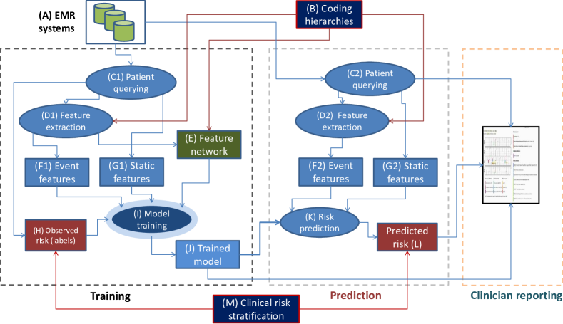
Figure 1: Overview of the automated medical risk stratification framework. Models are updated offline on a regular basis, prediction is made online at clinician’s request. The clinician reporting system is described elsewhere [52].

The framework is built on the patient-specific data queried from the relational EMR systems (denoted as A in Fig. 1). Patient data contains time-stamped events (such as emergency visits, diagnoses, and hospitalizations) and static information (such as gender, spoken language and occupation). For each patient, there are one or several evaluation points from which future risk will be predicted (Fig. 2). Often clinical risk assessments, hospital admissions or discharges serve as natural evaluation points as the outcomes will be tracked and acted upon.

The feature extraction process (D1,D2) generates event features (F1,F2) over multiple periods of times prior to an evaluation point (Section 4.2). The extraction process makes use of pre-defined coding hierarchies (B) such as the international disease coding scheme ICD-10 and the Australian intervention coding scheme ACHI. In the training phase, the process also generates a feature network (E) which encodes the temporal and semantic relations between features. For example, if depressive episodes were observed twice in the history, then the two features representing them are temporally linked. On the other hand, if another mental disorder is also observed, then the two disorders as semantically linked. The feature network will be used later on to improve the model stability.

The feature extraction process effectively flattens the structured EMRs into vectors, however temporal and hierarchical information is partially preserved. This process typically produces a large pool of features, and thus a feature selection capacity is needed. This is realized through model training (I) with lasso-style regularization [61]. More formally, let $\mathcal{D}=\left\{\boldsymbol{x}_{i},y_{i}\right\}_{i=1}^{n}$ be the training data set, where $\boldsymbol{x}_{i}\in\mathbb{R}^{d}$ denotes the feature vector of data instance $i$ and $y_{i}\in\left\{1,2,..,L\right\}$ the discrete ordinal output. We aim to learn a sparse, linear risk model parameterized by the weight vector $\boldsymbol{w}\in\mathbb{R}^{d}$. The lasso-regularized loss function is as follows:

$$\mbox{loss}_{1}(\boldsymbol{w})=\frac{1}{n}\sum_{i=1}^{n}R(\boldsymbol{x}_{i},y_{i};\boldsymbol{w})+\alpha\left\|\boldsymbol{w}\right\|_{1}$$ (1)

where $R(\boldsymbol{x}_{i},y_{i};\boldsymbol{w})$ is a convex loss function of training instance $i$ and $\alpha>0$ is the regularization parameter. To accommodate ordered risk classes, we employ several probabilistic ordinal classifiers what make different assumptions about the stratification process (Section 5). The loss function $R(\boldsymbol{x}_{i},y_{i};\boldsymbol{w})$ is therefore the negative log-likelihood of the outcomes $y_{i}$ given the features $\boldsymbol{x}_{i}$.

Model Stabilization Using Feature Network

The lasso tends to result in sparse models with few non-zeros weights. However, we observed that this sparsity typically comes with instability of the model under the random sampling of the training data $\mathcal{D}$. Model instability under feature selection is indeed a known phenomenon [6], but the theoretical study under lasso is recent [41].

The method proposed in this paper is based on the intuition that strong prior knowledge would lead to less variation due to sampling noise since prior knowledge is independent of sampling procedures. In clinical domains, prior knowledge could be realized by using feature networks, exploiting the relations between diseases and disease progression over time. In Fig. 1, the feature network (E) links related features and ensures that similar features have similar weights. This can be nicely formulated in a Bayesian regularization fashion as the feature network serves as a backbone for a precision matrix of the multivariate Gaussian prior distribution. Section 6 presents the network regularization in more details.

4 Representing Medical Data

This section describes the data and the process of transforming the temporal, hierarchical and relational EMR into flat feature vectors.

4.1 EMR Data

We are mainly interested in data on emergency department presentations (ED) and admissions to the general hospital. The most important piece of information is the diagnostic coding for any episodes. For ease of exposition we assume that the diagnosis coding conforms with the latest classification scheme, the ICD-10. Previous version or other schemes could be also be applicable. The ICD-10 scheme is a hierarchy of diseases covering almost all known conditions with approximately $20,000$ codes. The codes start with a letter followed by several digits where the digits placed later in the sequence indicate more specific conditions. For example, injuries to the head are classified into 10 groups, from S00 to S09. The group S01 means “open wound of head”, the subgroup S011 means “wound in the eyelid and periocular area”.

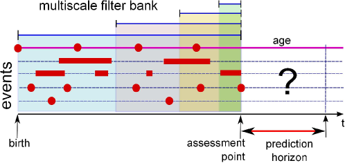
Figure 2: Clinical events represented as a temporal image, which is convoluted with one-sided filter bank.

In general, medical records for each patient contain time-stamped events of different types. Thus the EMR at a given time can be represented as a sparse 2D image (see Fig. 2). One dimension is time and the other dimension represents events. The events are sparse and irregular because clinical events are often packed into episodes. A typical episode starts with an emergency visit followed hospitalization and ends with discharge or death. For certain conditions such as mental health and cancers, formal risk assessments may be performed. Emergency visits, hospitalizations and risk assessments are major events that contain sub-events. For example, each emergency visit includes a primary ICD-10 diagnosis code, a decision to admit, transfer or return home. Hospitalization could be planned or come through the emergency department. Each admission typically contains multiple diagnoses, intervention procedures and medication prescriptions. A risk assessment may contain a check list or ordinal ratings on multiple risk-related items.

4.2 Multiscale Feature Extraction using One-Sided Filter Bank

Our prediction problem is to stratify future risk within a window of time using historical records. Thus at a prediction point, we transform the EMR into a feature vector to which risk classifiers are applied. As medical events are irregular and sparse, standard feature extraction techniques that rely on precise timing may not be robust. Instead, we exploit the 2D temporal image representation using a bank of one-sided filters. The concept resembles filters in signal processing and vision, except that the “signals” are sparse and irregular, also no future information will be used as the filter is one-sided.

Let $t$ be the time point of interest, $H$ be the maximum history length. Let $v_{j}(t)$ be the observation of the event of type $j$ at time $t$, for $j=1,2..,D$. Discrete events such as diagnosis are typically binary, i.e., $v_{j}(t)$ are the presence or absence of a code. For continuing events such as treatment episodes, $v_{j}(t)$ is the event duration. Let $\mathcal{K}^{k}(t;\sigma_{k})$ be a kernel function of $t$, parameterized by $\sigma_{k}$ and right-truncated at $0$ – that is, $\mathcal{K}^{k}(t;\sigma_{k})=0$ for $t\geq 0$. The $k$-th feature evaluated at $t$ for event $j$ is defined using the following convolution operation:

$$x_{j}^{k}(t)=\sum_{h=0}^{H}\mathcal{K}^{k}(s_{k}-h;\sigma_{k})v_{j}(t-h)$$ (2)

where $0\leq s_{k}\leq H$ denotes the delay. When $s_{k}=0$, the kernel is effective at anytime before time $t$. In effect, the event sequence of type $j$ is summarized throughout the history of length $H$ by the convolution operation. However, when $s_{k}>0$, the kernel is ineffective until $h\geq s_{k}$. This is equivalent to evaluating the feature at $t-h$, and thus this captures the temporal progression from $t-h$ to $t$.

The adjustable kernel parameter $\sigma_{k}$ controls the effective range of the kernel. This is important to differentiate acute conditions (such as suicide ideation) from chronic conditions (such as Type I diabetes). One useful kernel is the truncated Gaussian

$$\mathcal{K}^{k}(h;\sigma_{k})=\sqrt{\frac{2}{\pi\sigma_{k}^{2}}}\exp\left(-\frac{h^{2}}{2\sigma_{k}^{2}}\right)$$ (3)

where $\mathcal{K}^{k}(h;\sigma_{k})>0$ for $h\geq 0$ and $0$ otherwise. The hyper-parameter $\sigma_{k}$ defines the effective width of the kernel, i.e., the response drops drastically as $h$ goes beyond $\sigma_{k}$. The behavior is similar to the uniform kernel with specified width $\sigma_{k}$

$$\mathcal{K}^{k}(h;\sigma_{k})=\frac{1}{\sigma_{k}}\mathbf{1}\left[h\in[0,\sigma_{k}]\right]$$ (4)

This kernel counts the normalized number of events falling within a given period of time. Wavelet-like kernels could also be used to detect the trends and recurrences.

5 Modeling Ordinal Risk

We describe a set of ordinal regression models of risk associated with loss functions $R(\boldsymbol{x}_{i},y_{i};\boldsymbol{w})$ as in Eqs. (1). We assume that the observed outcomes $y\in\{1,2,...,L\}$ are the discretized version of underlying random risks $z\in\mathbb{R}^{m}$. The probabilistic models are natural to estimate the probability of a particular risk class being observed. Maximum likelihood learning leads to the risk $R(\boldsymbol{x}_{i},y_{i};\boldsymbol{w})=-\log P(y_{i}\mid x_{i};\boldsymbol{w})$. Two set of classifiers are presented: classifiers with and without shared parameters.

5.1 Models with Shared Parameters

For now we assume that all the classes share the same set of parameters $\boldsymbol{w}$. Relaxation will be considered in the next subsection.

5.1.1 Cumulative Classifier

This model assumes that the discrete outcomes $y$ are generated from the one-dimensional underlying random risk $z\in\mathbb{R}$ as follows [40]:

$$y = \begin{cases}1&\quad\mbox{if}\quad z\leq\tau_{1}\\ l&\quad\mbox{if}\quad\tau_{l-1}<z\leq\tau_{l}\\ L&\quad\mbox{otherwise}\end{cases}$$

where $\tau_{1}\leq\tau_{2}\leq...\tau_{L-1}$ are thresholds. This essentially says that the discrete outcome is a coarse version of the real-valued risk. The risk spectrum is the real line divided into intervals, each of which determines the corresponding outcome. In the form of probability distribution we have:

$$P(y=l\mid\boldsymbol{x}) = P(\tau_{l-1}\leq z\leq\tau_{l}\mid\boldsymbol{x})$$

$$= F(\tau_{l}\mid\boldsymbol{x})-F(\tau_{l-1}\mid\boldsymbol{x})$$

where $F(\tau_{l}\mid\boldsymbol{x})$ is the cumulative distribution evaluated at $\tau_{l}$. Choosing the form of $F(\tau_{l}\mid\boldsymbol{x})$ is usually the matter of practical convenience since $x$ is unobserved and we do not know the true underlying distribution. For example, the logistic distribution $F(\tau_{l}\mid\boldsymbol{x})=\left[1+\exp\left(-(\tau_{l}-\boldsymbol{w}^{\top}\boldsymbol{x})\right)\right]^{-1}$has an interesting interpretation:

$$\log\left(\frac{P(r\leq l\mid\boldsymbol{x})}{P(r>l\mid\boldsymbol{x})}\right)=\tau_{l}-\boldsymbol{w}^{\top}\boldsymbol{x}$$

i.e., the log odds at the split level $l$ is proportional to the risk factors. . The parameters to be estimated are $\boldsymbol{w}$ and $\left\{\tau_{l}\right\}_{l=1}^{L-1}$.

5.1.2 Stagewise Classifier

Cumulative models assume a single risk variable that can explain the ordinal outcomes. This assumption does not address the nature of the risk progression – for some patients, the risk may not reach a certain level immediately. It may, alternatively, start from a normal condition, and then progress upward. This suggests a stagewise model of outcomes. The next outcome level may be attained only if the lower levels have not been attained [65, 63]. The stagewise process can be formalized as follows:

$$y = \begin{cases}1\quad&\mbox{if}\quad z_{1}\leq\tau_{1}\\ l\quad&\mbox{if}\quad\left\{z_{m}\geq\tau_{m}\right\}_{m=1}^{l-1}\,\&\,z_{l}\leq\tau_{l}\\ L\quad&\mbox{otherwise}\end{cases}$$

where $m=1,2,..,l-1$ is the index of the risk levels below the current level $l$. Here, the transition from level $l$ to level $l+1$ is signified by the event that the risk value passes through the level-specific threshold $\tau_{l}$. The probability that the outcome is the lowest is then given as:

$$P(y=1) = P(z_{1}\leq\tau_{1})=F(\tau_{1})$$

If the condition $z_{1}\leq\tau_{1}$ does not hold, then we consider level $2$,

$$P(y=2\mid z\geq 2) = P(z_{2}\leq\tau_{2})=F(\tau_{2})$$

This process continues until some level has been accepted, or we must accept the last level $L$. Thus the probability of having the highest level of risk, given all the lower levels have not been accepted, is

$$P(y=L\mid y>L-1)=1-F(\tau_{L-1})$$

As all the decision steps rely on the same distribution $F(\tau)$, it is natural that $\tau_{1}<\tau_{2}<...<\tau_{L-1}$.

Note that the probabilities above are conditional. The marginal probability of selecting a particular discrete outcome is

$$P(y=l)=\begin{cases}F(\tau_{1})&\mbox{if }l=1\\ F(\tau_{l})\prod_{m=1}^{l-1}\left(1-F(\tau_{m})\right)&\mbox{if }l\in\{2,..,L-1\}\\ \prod_{m=1}^{L-1}\left(1-F(\tau_{m})\right)&\mbox{otherwise}\end{cases}$$

With the choice $F(\tau_{l})$ as a logistic distribution, we have a nice interpretation

$$\log\left(\frac{P(y=l\mid\boldsymbol{x})}{P(y\geq l\mid\boldsymbol{x})}\right)=\tau_{l}-\boldsymbol{w}^{\top}\boldsymbol{x}$$

i.e., the log odds of the probability of choosing the next level, given that all previous levels have failed, is proportional to the risk factors $\boldsymbol{x}$. Similar to the case of cumulative models, the parameters to be estimated are $\boldsymbol{w}$ and $\left\{\tau_{l}\right\}_{l=1}^{L-1}$.

5.2 Models with Separate Parameters

Models with shared parameters described in the previous subsection treat outcome risk as one-dimensional. However, risk classes could be qualitatively different – for example, some people never cross the line from an attempted suicide to a completed suicide. This suggests treating risk classes with separate parameter sets. In general, we have $L-1$ parameter sets $\mathbf{w}=\left\{\boldsymbol{w}_{1},\boldsymbol{w}_{2},...,\boldsymbol{w}_{L-1}\right\}$.

Let us return to the stagewise model studied in Sec. 5.1.2. Since there are several stages, we need not assume that there is only one underlying risk distribution. Instead, class-specific risk distribution $F_{l}(\tau_{l};\boldsymbol{w}_{l})$ can be used, where each class has their own parameter $\boldsymbol{w}_{l}$ and threshold $\tau_{l}$ for $l=1,2,...,L-1$. The marginal distribution is then:

$$P(y=l)=\begin{cases}F(_{1}\tau_{1})&\mbox{if }l=1\\ F_{l}(\tau_{l})\prod_{m=1}^{l-1}\left(1-F_{m}(\tau_{m})\right)&\mbox{if }l\in\{2,..,L-1\}\\ \prod_{m=1}^{L-1}\left(1-F_{m}(\tau_{m})\right)&\mbox{otherwise}\end{cases}$$

6 Stabilizing Predictive Models

Under lasso-regularized training (Eq. (1)), the selected features and their weights form a model. Unfortunately, under the sparsity constraints, models may be unstable under data variations. The medical domain amplifies this problem even more. First, features extracted from EMR (see Sec. 4.2) are highly redundant and correlated. Lasso-based regularization, however, tends to select only one feature between two strongly correlated ones [72]. Second, as features are often weakly predictive, their selection probability is usually less than $1$. When training data vary, this results in unstable models – the selected feature subset and their weights change significantly from one training setting to another. This instability is problematic in clinical settings because the learned model does not generalize from one cohort to another.

This section presents a remedy for this problem. First we define measures of model stability and show how to exploit existing relational structures in the data to stabilize the learned models.

6.1 Stability Indices

To quantify model stability, we assume that the models are trained on samples drawn randomly from an unknown data distribution $\hat{\mathcal{D}}\sim P(\mathcal{D})$ of the same size $n$. Each sample $b$ produces a set of features and their weights $\boldsymbol{w}^{b}$. Suppose that features are ranked through some criteria $\pi$, that is we have a sequence of features $\left\{x_{\pi(1)},x_{\pi(2)},...,x_{\pi(d)}\right\}$, we suggest two model stability indices:

• Averaged selection probability (ASP) at length $T$. This measures how strong the features are against both selection and ranking criteria, where $T\leq d$ is the length of the selected rank list:

  $$ASP@T=\frac{1}{T}\sum_{t=1}^{T}\sum_{\mathcal{D}}\mathbb{I}\left(w_{\pi(t)}^{\mathcal{D}}\neq 0\right)P(\mathcal{D})$$ (5)

  The term $\sum_{\mathcal{D}}\mathbb{I}\left(w_{\pi(t)}^{\mathcal{D}}\neq 0\right)P(\mathcal{D})$ is probability that a feature is selected [41]. This index is bounded within $\left[0,1\right]$.

• Averaged signal-to-noise ratio (SNR) at length $T$. Assume that the mean and standard deviation of feature weights are $\left\{\left(\bar{w}_{j},\sigma_{j}\right)\right\}_{j=1}^{d}$. The average SNR at $T$ is defined as:

  $$SNR@T=\frac{1}{T}\sum_{t=1}^{T}\frac{\left|\bar{w}_{\pi(t)}\right|}{\sigma_{\pi(t)}}$$ (6)

  When no regularization is imposed, the SNR square is the well-known Wald statistic.

In practice, since $P(\mathcal{D})$ is unknown, we propose to draw $B\gg 1$ random sets from the original set $\mathcal{D}$. One way is using bootstrap [18] in that each set is resampled with replacement. Alternatively, we can subsample $50\%$ of the data [41]. The $ASP@T$ reduces to $ASP@T=\frac{1}{TB}\sum_{t=1}^{T}\sum_{b=1}^{B}\mathbb{I}\left(w_{\pi(t)}^{b}\neq 0\right)$. The $SNR@T$ stays in the same form given that mean and standard deviations $\left\{\left(\bar{w}_{j},\sigma_{j}\right)\right\}_{j=1}^{d}$ are estimated from the samples.

The next issue is the ranking criteria $\pi$. Selection probability [41] and the individual SNR $\frac{\left|\bar{w}_{j}\right|}{\sigma_{j}}$ could be natural criteria. Under the regression framework, one can also employ the importance score [21] as:

$$I_{j}=\left|\bar{w}_{j}\right|\mbox{std}(x_{j})$$ (7)

where $\mbox{std}(x_{j})$ is the standard deviation of $x_{j}$. The importance is largely scale-invariant.

6.2 Stabilizing Sparse Models using Relational Structures

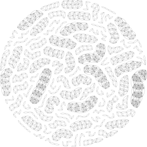
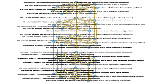
(a) ICD-10 code network	(b) Mental health sub-network

Figure 3: (a) Feature sub-networks for ICD-10 diagnoses from a mental health cohort when a $2$-character sharing is counted as a link. (b) Subnet of mental health diagnoses. Fully connected cliques are for related codes in the same extraction period. As example, one clique in (b) represents the group (F10-F13,F15,F17,F19) (Mental and behavioral disorders due to psychoactive substance use). Rare diagnoses are not presented. See Section 7.1 for data description.

To stabilize models, we exploit known structures in the features. The first structure is temporal, wherein each event type is evaluated at different time-scales and points, as parameterized by the kernel width $\sigma_{k}$ and the delay $s_{k}$ in Eq. (2) respectively. The other structure is the coding hierarchy, where the code is either a diagnostic code, procedure, DRG or medication class. The common property of the two structures is the relation among features of the same type. For simplicity, we do not distinguish between relations due to time-scale and those due to delay. Further, any two codes that share the same prefix are considered to be correlated. See Fig. 3 for the sub-network of diagnostic codes used in the experiments.

Let $W\in\mathbb{R}^{n\times n}$ be the nonnegative matrix that encodes the relation between features, i.e., $W_{ij}>0$ if features $i$ and $j$ are related and $W_{ij}=0$ otherwise. Let $S=g(W)\in\mathbb{R}^{n\times n}$ be some transform of the relation matrix into the correlation matrix. When all classes share the same parameter set (Section 5.1), the loss function in Eq. (1) is modified as follows:

$$\mbox{loss}_{2}(\boldsymbol{w})=\frac{1}{n}\sum_{i}R(\boldsymbol{x}_{i},y_{i};\boldsymbol{w})+\alpha\left\|\boldsymbol{w}\right\|_{1}+\beta\boldsymbol{w}^{\top}S\boldsymbol{w}$$ (8)

where $\beta>0$ is the correlation parameter.

When $S$ is semi-definite positive, this is equivalent to a compound prior of a Laplace and a Gaussian of mean $\boldsymbol{0}$ and covariance matrix of $\beta S^{-1}$. Minimizing the loss could be interpreted as finding maximum a posterior (MAP) solution. Let $\Omega(\boldsymbol{w};S)=\boldsymbol{w}^{\top}S\boldsymbol{w}$, we discuss two interesting transforms from $W$ to $S$:

• Linear association. This assumes that correlation is a linear function of relation, that is $S=D-W$, where $D$ is a positive diagonal matrix. This translates to the regularizer:

  $$\Omega(\boldsymbol{w};S)=\sum_{j}D_{jj}w_{j}^{2}-\sum_{j}\sum_{k}W_{jk}w_{j}w_{k}$$

  Thus minimizing the loss tends to encourage positive correlation between paired feature weights. The quadratic term in the left hand side is needed to prevent the weights from going too large. One special case is the Laplacian smoothing [34, 20], where $D_{jj}=\sum_{k}W_{jk}$, and the above equation can be rewritten as:

  $$\Omega(\boldsymbol{w};S) = \sum_{j}\left(\sum_{k}W_{jk}\right)w_{j}^{2}-\sum_{j}\sum_{k}W_{jk}w_{j}w_{k}$$ (9)

  $$= \frac{1}{2}\sum_{jk}W_{jk}\left(w_{j}-w_{k}\right)^{2}$$

  This regularizer treats all the relations equally.

• Random walk. Assume that $W$ is a probabilistic matrix, i.e., $\sum_{k}W_{jk}=1$ for all $j$, $W_{jk}$ is the probability of random walk from “state” $j$ to state $k$. This suggests the following regularizer [56]:

  $$\Omega(\boldsymbol{w};S) = \sum_{j}\left(w_{j}-\sum_{k}W_{jk}w_{k}\right)^{2}$$ (10)

  $$= \boldsymbol{w}^{\top}(I-W)^{\top}(I-W)\boldsymbol{w}$$

  where $I$ is the identity matrix. That is, $S=(I-W)^{\top}(I-W)$, which is symmetric nonnegative definite. This regularizer distributes the smoothness equally among all features.

The Laplacian and random walk regularizations encourage correlated features to have similar weights. This prevents the cases where only one in a group of strongly correlated, predictive features is selected by sparsity methods [67]. The $\ell_{1}$ regularizer, however, effectively pushes weaker feature groups toward zero weights. The overall effect is that strong feature groups are more frequently selected, but weak feature groups have less chance compared to the case without network regularization. Thus the effect bears some similarity with the sparse group methods [70]. The difference is that our method is much more flexible with correlation structures such as non-overlapping grouping.

The extension to the case of class-specific parameters (Section 5.2) is straightforward:

$$\mbox{loss}_{3}(\mathbf{w})=\frac{1}{n}\sum_{i}R(\boldsymbol{x}_{i},y_{i};\mathbf{w})+\sum_{l=1}^{L-1}\left(\alpha\left\|\boldsymbol{w}_{l}\right\|_{1}+\beta\boldsymbol{w}_{l}^{\top}S_{l}\boldsymbol{w}_{l}\right)$$ (11)

For simplicity we assume that $S_{l}=S$ for all $l=1,2,...,L-1$ although $S_{l}$ can encode class-specific prior knowledge (e.g., diabetes and hypertension are correlated under the high-risk scheme).

7 Implementation and Results

This section details an real-world application of the proposed framework for suicide risk prediction. The cohort under study consists of mental health patients who were under suicide risk assessments. Suicide stratification has been widely acknowledged to be extremely difficult for clinicians as there are a large number of possible risk factors but none of them are strong enough [55]. This has led to recent doubts that predictive models may not be useful at all [31].

7.1 Data

7.1.1 Mental Health Dataset

We collected the EMR data from Barwon Mental Health, Drugs and Alcohol Services, the only provider in the region of 350,000 people in the central western region of Victoria in South-eastern Australia. For emergency attendances (ED), there are $42K+$ recorded mental cases for $8K+$ patients in the period of 2005–2012. For hospital admissions (HA), there are approximately $67K$ recorded mental cases in the period of 1995–2012. The number of recorded emergency attendances and admissions has increased over the years, e.g., from 7,068 admissions in 2009 to 8,143 in 2010 and 8,956 in 2012. The hospitals perform suicide risk assessments for every mental patient under its care. The instrument has ordinal assessments for 18 items covering all mental aspects such as suicidal ideation, stressors, substance abuse, family support and psychiatric service history. The system recorded approximately $25K$ assessments on $10K$ patients in the period of 2009-2012. The majority of patients have only one assessment (62%), followed by two assessments (17%), but there are about 3% patients who have more than 10 assessments. For those with more than one assessment, the time between two successive assessments are: 30% within one week, 64% within 3 months.

We focus our study on those patients who have had a least one event prior to a risk assessment. The dataset then has $7,578$ patients and $17,566$ assessments. For each patient, we collect age, gender, spoken language, country of birth, religion, occupation, marital status, indigenous status, and the postcodes over time. Among patients considered, $49.3\%$ are male and $48.7\%$ are under 35 of age at the time of assessment.

The risk assessments are natural evaluation points for future prediction within a given window. Future outcomes are broadly classified into three levels of risk, based on a senior psychiatrist at Barwon Health: class $C_{1}$ refers to low-risk outcomes, class $C_{2}$ refers to moderate-risk (low lethality attempts), and class $C_{3}$ the high-risk (high lethality outcomes). The classes are assigned using a look-up table from the diagnosis codes.

The convention is that among all events occurring within the prediction period, the class of the highest risk is chosen. For example, the ICD-10 coded event S51 (open wound of forearm) is moderate-risk, while S11 (open wound of neck) would be considered as high-risk. Typically the completed suicides are rare, and the class distributions are imbalanced. For example, for 1-month period following the risk assessment, there are only $24$ suicides among $409$ lethal attempts ($2.3\%$), and $834$ moderate-risk attempts ($4.8\%$). Further class distributions are summarized in Table 1.

Horizon (day)	30	60	90	180
$C_{1}$	16,323	15,750	15,272	14,291
$C_{2}$	834	1,172	1,436	19,25
$C_{3}$	409	644	8,58	1,350
Suicide	24	32	41	63

Table 1: Outcome class distribution following risk assessments.

7.1.2 Data Preprocessing

The filter bank technique (Sec. 4.2) assumes that the discrete events are given. In addition to primitive events such as emergency visits, we use several derived events. First, ICD-10 codes and intervening procedures are mapped into their higher level codes in their corresponding hierarchies. For example, the code “F32.2” (Severe depressive episode without psychotic symptoms) would be mapped into “F32” if level 3 in the ICD-10 hierarchy is used. This is to make the feature list robust by reducing the number of rare codes. Second, diagnosis-related groups (DRGs) are computed from diagnoses and interventions taking into account of disease severity and treatment complexity. Following [44], we derive Mental Health Diagnosis Groups (MHDGs) from ICD-10 codes using the mapping table. The MHDGs offer an alternative view to the mental health code groups in the ICD-10 tree. Likewise, we also map diagnoses into 30-element comorbidities [19], as they are known to be predictive of mortality/readmission risk. From demographic data, postcode changes are tracked on the hypothetical basis that a frequent change could signify socio-economic problems.

For robustness we only consider separate items (e.g., codes) with more than $100$ occurrences. Other items that do not satisfy these conditions are considered rare events. Such rare events, though statistically less important, are critical in identifying risks if combined. We empirically find that using diagnostic features at level $3$ in the ICD-10 hierarchy gave the best result as they appears to balance generality and specificity. Similarly, for intervention procedures, we use code blocks instead of detailed codes.

The convolution operators in the filter bank (Section 4.2) could be applied several times to obtain compound sum/mean statistics. The filters, however, do not support min/max statistics. Medical risks, on the other hand, are of great importance at the extreme, suggesting the use of max operators. For example, out of risk items in an assessment, an extreme risk would be sufficient to raise the alarm. Similarly, for an item, an extreme value within the last 3 months would suggest serious surveillance even though the current assessment is moderate. Thus we create an extra subset of features with the max statistics, as listed in Table 2.

(i)	Max of (overall ratings) over time
(ii)	Sum of (max ratings over time) over 18 items
(iii)	Sum of (mean ratings over time) over 18 items
(iv)	Mean of (sum ratings over 18 items) over time
(v)	Max of (sum ratings over 18 items)

Table 2: Derived features from risk assessments. Features (iii,iv) can be obtained by applying the filters twice, one over time, the other over items.

7.2 Implementation

#Ordered levels	3
#Patients	7,578
#Data points	17,566
#Features	5,376
#Edges in feature network	79,072

Table 3: Data statistics.

7.2.1 Feature Extraction and Network Construction

We choose uniform kernels for ease of interpretation with the following scale/delay pairs: $\left(\sigma_{k};s_{k}\right)\in\left\{\left(3,0\right);\left(3,3\right);\left(6,6\right);\left(12,12\right);\left(24,24\right)\right\}$ (months), see also Eq. (2). This means that the $4$-year history is divided into non-overlapping segments: {$[0-3]$,$[3-6]$,$[6-12]$,$[12-24]$,$[24-48]$} (months). The segment size increases from the most recent to the distant past, and this encodes the belief that old information is less specific to the current health state. Filter responses are then normalized into the range [0,1] and then squared.

The construction of feature network follows feature extraction. We consider two types of network relations: Same-Code (any two features corresponding to the same code at different extraction periods), and Shared-Ancestor (any two codes that belong to the same branch in their code hierarchy and the same extraction period). There are four coding types: diagnoses, intervention procedures, MHDGs, DRGs, and medications. For each coding type, the first two characters and digits are used to identify the Shared-Ancestor relation. For example, diagnosis code F31 (Bipolar affective disorder) and F32 (Depressive episode) would be linked, but F31 and F20 (Schizophrenia) would not. The resulting network has $5.4K$ nodes and $97.1K$ edges. Fig. 3(a) shows the entire ICD-10 network (less the rare diagnoses), and Fig. 3(b) displays the sub-network corresponding to mental health diagnoses. Table 3 summarizes the statistics of the data.

7.2.2 Learning Classifiers

For cumulative and stagewise classifiers (Sec. 5.1.1 and Sec. 5.1.2), logistic distributions for the underlying random risks are used. We approximate the $\ell_{1}$-norm $|x|$ in Eqs. (1,8,11) by the Huber-like loss function, where $H(w)=0.5w^{2}/\epsilon$ if $|w|\leq\epsilon$ and $H(w)=|w|-0.5\epsilon$ otherwise for some small $\epsilon>0$. This loss function behaves like $|w|$ when $|w|$ is large compared to $\epsilon$. However, the gradient is smooth: $H^{\prime}(w)=w/\epsilon$ if $|w|\leq\epsilon$ and $H^{\prime}(w)=\mbox{sign}(w)$ otherwise. This makes it possible to use fast large-scale optimization algorithms such as L-BFGS. Once the optimization has converged, features are selected if their absolute weights are larger than $10^{-3}$.

7.2.3 Evaluation Protocol

We use $10$-fold cross-validation in the patient space, that is, the set of unique patients is divided in to subsets of equal size. Classifiers are trained on data for $9$ subsets and tested on the remaining subset. The results are reported for all validation subsets combined. Note that this can be a stronger test than the cross-validation in the data space because it removes any potential patient-specific correlation (also known as random-effects). We employ several performance measures: For each outcome class, we use recall $R$ – the portion of groundtruth class that is correctly identified; the precision $P$ – the portion of identified class that is actually correct; and the F-score – their harmonic mean $F_{1}=2RP/(R+P)$. While these measures are appropriate for class-specific performance, they do not represent misclassification in the ordinal setting well. For that reason, we also use Macro-averaged Mean Average Error (Macro-MAE) [4] – the discrepancy between the true and the predicted risk levels, adjusted for data imbalance.

7.3 Risk Prediction

7.3.1 Sensitivity to Hyperparameters

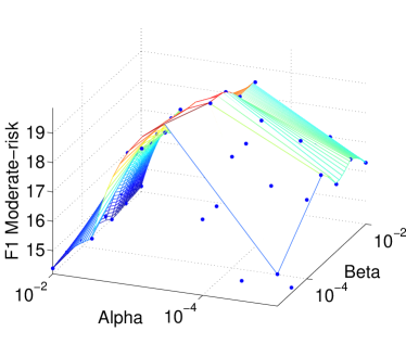
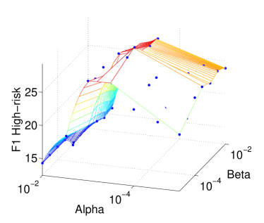
(a) Moderate-risk	(b) High-risk

Figure 4: Performance ($F$-scores) of the cumulative classifier (Section 5.1.1) against hyperparameters in Eq. (8): $\alpha$ (sparsity) and $\beta$ (stability, using Laplacian methods, Eq. (9)). $\beta=0$ reduces to standard lasso-based sparse models. Similar behaviors are also observed with other classifiers.

There are two hyperparameters in our objective function in Eq. (8): the $\ell_{1}$-norm regularization factor $\alpha$ and the network regularization factor $\beta$. These two factors serve different purposes: The $\ell_{1}$-norm regularization as an embedded feature selection mechanism, and the network regularization for stabilizing the models. To investigate the sensitivity of the final performance against these hyperparameters, we perform a grid search in the set {$10^{-5},$$3\times 10^{-5}$,$10^{-4}$,$3\times 10^{-4}$,$10^{-3}$,$3\times 10^{-3}$,$10^{-2}$} for each. Figs. 4(a,b) report the $F_{1}$-score measures for the moderate-risk ($C_{2}$ class) and high-risk ($C_{3}$ class) outcomes within $3$ months under cumulative classifiers (Section 5.1.1). The $F_{1}$-scores in both risk classes critically depends on $\alpha$ but are relatively stable against $\beta$. The former dependency is expected: large $\alpha$ generally leads to sparser models, and thus less overfitting. When the sparsity reaches the right level – at $\alpha=3\times 10^{-4}$ – the predictive power peaks. The small effect of $\beta$ on the performance is interesting but not surprising. As large $\beta$ forces linked features to have similar weights, the feature influence is rearranged but overall their total effect remains largely unchanged. Thus in what follows, unless specified otherwise, we fix the sparsity hyperparameter as $\alpha=3\times 10^{-4}$ for all classifiers.

7.3.2 Comparison Against Clinicians

		$C_{2}$				$C_{3}$
	Macro-MAE	Cases	$R$	$P$	$F_{1}$	Cases	$R$	$P$	$F_{1}$
Clinician	0.826	338	23.5	11.7	15.6	70	8.2	12.9	10.0
CUMUL	0.675	429	29.9	14.8	19.8	282	32.9	26.0	29.0
STW (Shared)	0.681	417	29.0	14.4	19.3	263	30.7	25.6	27.9
STW (Multi)	0.672	418	29.1	14.5	19.3	289	33.7	26.7	29.8

Table 4: Predicting 3-month risk on EMR data without model stabilization (standard sparse models). $C_{2}$ = moderate-risk, $C_{3}$ = high-risk, $R$ = Recall, $P$ = Precision, in percentages. CUMUL = Cumulative model, STW = Stagewise model.

We first evaluate the predictive power of the mandatory risk assessments being performed by Barwon Health. Using the overall assessment (risk ratings of $3$ and $4$ are high-risk, $2$ moderate-risk, and ratings of $1$ and $0$ are low-risk), the performance on the high-risk class for $3$ month horizons is quite poor: $R=8.2\%$, $P=12.9\%$, $F_{1}=10.0\%$. There are $14$ suicide cases ($34\%$) detected from the $C_{2}$ and $C_{3}$ assignments. Tab. 4 lists more details. Machine learning algorithms applied to EMR data significantly outperform the mental health professionals to a large margin. For moderate-risk prediction, the $F_{1}$-score by machines reach roughly $19.5\%$, which are $25\%$ improvement over the score by clinicians. The differentials are even better for the high-risk class: the improvement are more than $180\%$. When accounting for class imbalance (Table 1), machine learning models win by roughly $18\%$ on the Macro-averaged MAE measure.

	Suicide	Resource	FN
	(out of 41)	cost ($\uparrow\%$)	($\downarrow\%$)
Clinician	14	3,444 (0.0)	1,530 (0.0)
CUMUL	30	3,821 (10.1)	1,309 (29.5)
STW (Shared)	29	3,920 (13.8)	1,138 (38.8)
STW (Multi)	29	3,973 (15.4)	1,108 (40.4)

Table 5: Predicting 3-month risk on EMR data without model stabilization (standard sparse models). CUMUL = Cumulative model, STW = Stagewise model. Resource cost is the total number of cases assigned as moderate/high-risk. FN = false negatives, which are the risky cases wrongly classified as low-risk. The symbols $\uparrow$ and $\downarrow$ denote the amount increase or decrease relative to the reference figures by clinicians.

The practical significance of the difference is remarkable. Assuming for simplicity that the management cost, on average, is similar for both the moderate and high risk classes. Thus a detection of moderate or high risk costs one basic resource unit. The machine algorithms typically use slightly more resource units than clinicians but with less false negatives (Table 5). For example, the stagewise classifier with shared parameters (Sec. 5.1.2) leads to $3,920$ resource units ($13.8\%$ higher than those by clinicians), but with $1,138$ false negatives ($25.6\%$ lower than those by clinicians). The significance may be amplified considering that the social cost for false negatives is much more serious than hospital resources. In terms of suicide detection, the machine detects $29-30$ cases, which are more than double the number detected by human ($14$ cases).

Next we examine whether using machine learning can improve the prediction using the risk assessments itself. We ran all classifiers on both assessment-based features, and EMR-based features using the Laplacian stabilization. The prediction horizons were 1,2, 3 or 6 months. As reported in Tables 6 and 7, machine learning methods trained on risk assessments consistently outperform clinicians. The results also demonstrate that using EMR alone is even better. This is significant because EMRs already exist in the data warehouse, that is, we can make predict without any extra cost.

		$C_{2}$				$C_{3}$
Classifier	Data	1mm	2mm	3mm	6mm	1mm	2mm	3mm	6mm
Clinician	RA	11.9	14.7	15.6	15.7	9.0	9.1	10.0	10.0
CUMUL	RA	13.1	16.0	17.4	19.3	13.3	16.2	20.0	25.3
	EMR	13.8	17.7	19.0	20.1	16.5	22.1	27.9	27.7
STW (Shared	RA	11.9	15.68	16.9	19.0	13.6	18.3	22.2	27.2
	EMR	13.8	18.4	19.2	19.9	16.7	25.4	29.4	30.9
STW (Multi)	RA	13.0	16.1	17.1	19.6	14.2	17.1	21.9	26.7
	EMR	14.0	17.4	19.5	20.6	16.7	22.5	28.4	29.7

Table 6: $F_{1}$-scores (%) at different prediction horizons (1,2,3,6 months). $C_{2}$ = moderate-risk, $C_{3}$ = high-risk, CUMUL = Cumulative model, STW = Stagewise model, RA = Risk assessments, EMR = Electronic Medical Record. Laplacian stabilization was used, $\alpha=3\times 10^{-3}$.

Classifier	Data	1mm	2mm	3mm	6mm
Clinician	RA	0.786	0.811	0.826	0.852
CUMUL	RA	0.727	0.735	0.735	0.745
	EMR	0.688	0.677	0.675	0.712
STW (Shared	RA	0.722	0.720	0.724	0.737
	EMR	0.671	0.655	0.681	0.704
STW (Multi)	RA	0.721	0.726	0.725	0.740
	EMR	0.670	0.682	0.672	0.705

Table 7: Macro-MAE at different prediction horizons (1,2,3,6 months). CUMUL = Cumulative model, STW = Stagewise model, RA = Risk assessments, EMR = Electronic Medical Record. Laplacian stabilization was used, $\alpha=3\times 10^{-3}$.

7.4 Model Stability

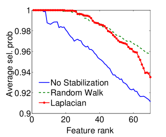
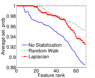
(a) Cumulative, $C_{2}+C_{3}$	(b) Stagewise (Shared), $C_{2}+C_{3}$
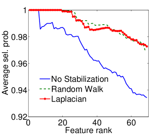
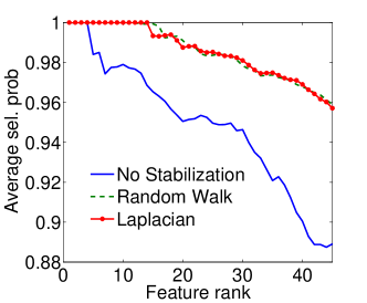
(c) Stagewise (Separate), $C_{2}$	(d) Stagewise (Separate), $C_{3}$

Figure 5: Average selection probability ($ASP@T$ – see Eq. (5)), evaluated at different rank list sizes (the larger probability, the more stable models). “No Stabilization” means the standard lasso framework with $\beta=0$. For others, $\alpha=3\times 10^{-4},\beta=3\times 10^{-3}$.

We now examine the models stability against data sampling and evaluate the stabilizing property of the proposed method (Sec. 6.2). For each fold, we generated $30$ samples, each of which was drawn randomly from $50$% of training data. Each example resulted in a model, and the feature weights were recorded and finally the results of all $10$ folds – $300$ models – were combined. Figs. 5(a–d) show the $ASP@T$ indices (Eq. (5)) as functions of the rank list size $T$, for all ordinal classifiers. The instability is clearly an issue – the average selected probability drops as more features are included. Using both the Laplacian and random walk regularization methods (Eqs. (9,10)), the improvement in stability is evidenced in all settings. The instability and stabilizing effect were similarly obtained with the $SNR@T$ indices (Figs. 6(a–d)).

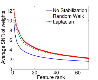
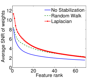
(a) Cumulative, $C_{2}+C_{3}$	(b) Stagewise (Shared), $C_{2}+C_{3}$
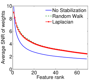
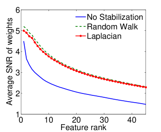
(c) Stagewise (Separate), $C_{2}$	(d) Stagewise (Separate), $C_{3}$

Figure 6: Average signal-to-noise ratio ($SNR@T$– see Eq. (6)), evaluated at different rank list sizes (the larger average SNR, the more stable model). “No Stabilization” means the standard lasso framework with $\beta=0$. For others, $\alpha=3\times 10^{-4},\beta=3\times 10^{-3}$.

7.5 Discovered Features

Feature	($\sigma_{k};s_{k}$)	Importance	SNR
Number of EDs	($3;0$)	59.6	8.5
Number of EDs	($3;3$)	32.5	6.6
Moderate-lethality attempts ($C_{2}$)	($12;12$)	10.9	5.1
Moderate-lethality attempts ($C_{2}$)	($6;6$)	9.1	4.1
High-lethality attempts ($C_{3}$)	($3;0$)	14.6	4.4
Moderate-lethality attempts ($C_{2}$)	($24;24$)	12.1	4.4
Number of EDs	($6;6$)	22.6	4.3
Number of postcode changes & Male	($3;0$)	26.0	4.0
High-lethality attempts ($C_{3}$)	($3;3$)	10.3	4.0
ICD code: F19 (Mental disorders due to drug abuse)	($6;6$)	9.8	3.8
ICD code: Z91 (History of risk-factors, unclassified)	($24;24$)	9.0	3.6
High-lethality attempts ($C_{3}$)	($6;6$)	8.0	3.3
ICD code: T50 (Poisoning)	($3;0$)	14.6	3.2
ICD code: Z29 (Need for other prophylactic measures)	($3;0$)	24.0	3.2
Number of postcode changes & Male	($3;3$)	10.8	3.0
Comorbidity: Alcohol abuse	($6;6$)	5.2	2.9
Number of EDs	($12;12$)	12.6	2.8
ICD code: S06 (Intracranial injury)	($3;0$)	2.9	2.7
ICD code: U73 (Other activity)	($3;0$)	6.8	2.5
ICD code: T43 (Poisoning by psychotropic drugs)	($3;0$)	7.4	2.5

Table 8: Top $20$ predictive and stable features associated with risky outcomes in the next $3$ months, ranked by signal-to-noise ratios, as produced by the stagewise classifier with shared parameters (Sec. 5.1.2), under Laplacian regularization (Eq. 9). The uniform kernel width $\sigma_{k}$ and the delay $s_{k}$ are measured in months; ED = Emergency Attendance, MHDG = Mental Health Diagnosis Group.

Cumulative classifiers and stagewise classifiers with shared parameters do not distinguish the parameters between classes and thus we have a single list of features at the end of the training phase. Tab. 8 presents top $20$ features ordered by their SNRs, as produced by the stagewise classifier with shared parameters (Sec. 5.1.2). Predictive features include: Recent emergency visits, recent high-risk attempts ($C_{3}$), moderate-risk attempts ($C_{2}$ & self-poisoning) within 24 months, recent history of mental problems and of drug abuse, socioeconomic problems (frequent home moving).

Feature		($\sigma_{k};s_{k}$)	Importance	SNR
Moderate-risk class $(C_{2})$
	Number of EDs	($3;0$)	59.1	9.0
	Number of EDs	($3;3$)	32.9	7.3
	Moderate-lethality attempts ($C_{2}$)	($6;6$)	13.6	5.6
	Moderate-lethality attempts ($C_{2}$)	($12;12$)	13.7	4.9
	Number of EDs	($6;6$)	18.3	4.6
	Moderate-lethality attempts ($C_{2}$)	($24;24$)	15.6	4.3
	ICD code: Z91 (History of risk-factors, unclassified)	($24;24$)	8.5	4.1
	Comorbidity: Alcohol abuse	($6;6$)	7.0	4.1
	Moderate-lethality attempts ($C_{2}$)	($3;3$)	9.4	3.6
	Comorbidity: Alcohol abuse	($3;3$)	8.1	3.6
	Number of postcode changes & Male	($3;0$)	20.0	3.4
	ICD code: Z29 (Need for other prophylactic measures)	($3;0$)	28.2	3.3
	Moderate-lethality attempts ($C_{2}$)	($3;0$)	9.7	3.3
	Comorbidity: Alcohol abuse	($3;0$)	9.0	3.2
	ICD code: F19 (Mental disorders due to drug abuse)	($6;6$)	7.8	3.1
High-risk class $(C_{3})$
	ICD code: T43 (Poisoning by psychotropic drugs)	($3;0$)	24.0	5.0
	High-lethality attempts ($C_{3}$)	($3;0$)	30.6	4.8
	ICD code: T43 (Poisoning by psychotropic drugs)	($3;3$)	15.2	4.1
	High-lethality attempts ($C_{3}$)	($3;3$)	24.0	4.1
	ICD code: T42 (Poisoning by antiepileptic,	($3;0$)	15.3	3.6
	sedative-hypnotic and antiparkinsonism drugs)
	ICD code: U73 (Other activity)	($3;3$)	10.6	3.4
	ICD code: T42 (Poisoning by antiepileptic,	($3;3$)	11.0	3.2
	sedative-hypnotic and antiparkinsonism drugs)
	ICD code: T50 (Poisoning)	($3;0$)	17.3	3.1
	ICD code: X61 (Intentional self-poisoning)	($3;0$)	10.0	3.0
	Occupation: student & Female	NA	69.5	2.8
	High-lethality attempts ($C_{3}$)	($6;6$)	13.3	2.7
	ICD code: U73 (Other activity)	($3;0$)	11.4	2.7
	ICD code: X61 (Intentional self-poisoning)	($3;3$)	6.3	2.7

Table 9: Top $15$ predictive and stable features associated with risk classes in the next $3$ months, ranked by signal-to-noise ratios, as produced by the stagewise classifier without parameter sharing (Sec. 5.1.2). The uniform kernel width $\sigma_{k}$ and the delay $s_{k}$ are measured in months; MHDG = Mental Health Diagnosis Group.

Stagewise classifiers with class-specific parameters can offer re-ranking of features for $C_{2}$ and $C_{3}$ separately. Tabs. 9 list top-ranked class-specific features for $C_{2}$ and $C_{3}$, respectively, under the stagewise classifiers. A noticeable aspect is the strong association between prior $C_{3}$ attempts with future $C_{3}$ outcomes.

8 Discussion

Compared against existing work in medical risk models, our machine learning method is hypothesis-free, i.e., without collection bias nor prior assumptions about specific risk factors. As the model is derived from routinely collected administrative hospital data, it can be readily embedded into existing EMR systems. Second, as all available information is utilized, there is less chance that importance risk factors will be overlooked. In fact, the features we have just discovered (Tables 8 and 9) resemble ones well-documented in the clinical literature [10]. For example, male, socio-economic issues, psychiatric factors, previous attempts are known to be positively correlated with subsequent suicide attempts [22, 24, 39]. Factors distantly related to psychological distress such as prior hospitalization, ED visits or physical illnesses were also previously reported [15, 38, 51]. Our results, however, differentiate from the previous work since they are more precise in timing, and do not rely on hand-crafted prior hypotheses.

The result is significant as the discovery is essentially free and automated, as compared to expensive and time-consuming medical studies. However, as EMR data may contain noise and depend on system implementation, discovered risk factors may not totally universal, and our system thus should be used as a fast screening tool for further in-depth clinical investigation.

Unlike existing machine learning work applied to healthcare, our goal was to achieve not only high performance but also interpretability and reproducibility. The prediction is transparent and for each patient, it explains specific risk factors involved in the risk estimate, and how stable the risk factors are (Tables 8 and 9). Although feature stability has gained significant attention recently [3, 28], this has not been studied in the context of clinical prediction models. Further, we contribute to the literature two new stability indices, the ASP@T and SNR@T, where the SNR@T measures not only the feature stability but also its statistical significance (the Wald statistic). This statistic is largely ignored in data mining practice.

Our work demonstrated that model stability for high-dimensional problems could be significantly enhanced by exploiting known relations between features. This validates our intuition that prior knowledge would help as it is independent of data sampling procedures. Consistent with prior studies, our results confirm that such prior relations, as realized in feature network regularization, improve the generalization when no other regularization schemes are in place [20][56]. However, interestingly, when combined with lasso, their effect on predictive performance is insignificant, as shown in Fig. 4. It is surprising because model stability could potentially lead to better prediction stability, and which is a sufficient condition for generalization [9, 49]. This suggests that the two stability concepts may not be strongly correlated, as it is known that random forests, for example, can generate very different tree ensembles (model instability) but the end results can be quite stable (prediction stability).

This paper grew from an effort to predict suicide, following difficulty in practice at Barwon Health, Australia. However, this goal was quickly deemed impossible, partly because of the long-standing conjecture that suicide is clinically unpredictable [32, 30]. From the machine learning perspective, suicide is a rare event, and thus a robust estimation would require detailed clinical data from millions of mental health patients, which is an impractical task. Instead, the mental health literature has concentrated on predicting suicide attempts without stratifying lethality. However, it is possible that the mental processes in low-lethality attempts differ significantly from those in high-lethality attempts, as suggested in Table 9. In practice, clinicians would want to target the latter group because of the high chance of subsequent death. Thus our paper contributes to the literature by separating the lethality classes in an ordinal regression framework. The lesson is that when facing rare events, instead of predicting the events itself, we should target regions where the events are likely to occur. Another finding is that, in medical domains, machine learning systems are most useful when data is large, comprehensive and complex, the risk factors are abundant, time-sensitive but weakly predictive. This is because clinicians, in their busy practice, may not able to consider a large number of relevant factors in the distant history.

This study has several limitations. First the framework has only been validated on data from a single hospital and has not been independently tested by external investigators. However, the framework has been tested on a variety of medical problems and cohorts (results are reported elsewhere), and the results so far have been encouraging: The predictive performance either matches or exceeds the state-of-the-arts in the clinical literature, and the discovered features resembles most important reported risk factors from multiple prior studies. Second, our labels were not perfect: (i) labels were collected at Barwon Health alone and we did not track transfers or readmissions to other institutions; (ii) labels were based on ICD-10 diagnosis codes and these may not be perfectly accurate due to the coding practices. This suggests that our performance estimates are conservative.

9 Conclusion

We have proposed a stabilized sparse ordinal regression framework for future risk stratification. The objectives are deriving and validating predictive algorithms from the rich source of electronic health records, and at the same time, offering clear explanation on how prediction is made. Central to the work is discovery of stable subset of factors that are predictive of future risk. The framework has several novel elements: (i) two model stability indices; (ii) a stability-based feature ranking criterion; and (iii) feature network regularization where similar features are encouraged to have similar weights, under the lasso-based sparsity framework.

The framework introduced in this paper is generalizable as the information extracted from the data warehousing is standardized. The EMR-based models make no use of human resources, except for the risk definition done only once. Our framework has been validated on a challenging problem of predicting suicide risk against clinicians. We demonstrated in this paper that the proposed system could (a) discover risk factors that are consistent with mental health knowledge; (b) significantly outperform clinicians using just readily collected data in hospitals; and (c) exploit feature relations improved model stability significantly.

Work in progress is testing the framework on a series of other predictive problems: Risk of hospitalization/mortality in diabetes, stroke, COPD, mental health, heart failure, heart attack and pneumonia, and cancers. The framework has been adopted by the hospitals and deployment is underway. This poses an interesting research question: How can we deal with the situation where the physicians modify their treatment strategy based on the machine prediction, and thus alter the outcome, leading to the poorer match between the actual outcome and the predicted one?

Acknowledgments

We thank Ross Arblaster and Ann Larkins for helping data collections, Paul Cohen for providing management support for the project, Richard Harvey for risk stratification, Michael Berk and Richard Kennedy for valuable opinions, and the reviewers for helpful comments.

References

- [1] Gad Abraham, Adam Kowalczyk, Sherene Loi, Izhak Haviv, and Justin Zobel. Prediction of breast cancer prognosis using gene set statistics provides signature stability and biological context. BMC bioinformatics, 11(1):277, 2010.
- [2] Michael H Allen, Beau W Abar, Mark McCormick, Donna H Barnes, Jason Haukoos, Gus M Garmel, and Edwin D Boudreaux. Screening for suicidal ideation and attempts among emergency department medical patients: Instrument and results from the psychiatric emergency research collaboration. Suicide and Life-Threatening Behavior, 2013.
- [3] Peter C Austin and Jack V Tu. Automated variable selection methods for logistic regression produced unstable models for predicting acute myocardial infarction mortality. Journal of clinical epidemiology, 57(11):1138–1146, 2004.
- [4] Stefano Baccianella, Andrea Esuli, and Fabrizio Sebastiani. Evaluation measures for ordinal regression. In Intelligent Systems Design and Applications, 2009. ISDA’09. Ninth International Conference on, pages 283–287. IEEE, 2009.
- [5] Ralf Bender and Ulrich Grouven. Ordinal logistic regression in medical research. Journal of the Royal College of Physicians of London, 31(5):546–551, 1997.
- [6] Jinbo Bi, Kristin Bennett, Mark Embrechts, Curt Breneman, and Minghu Song. Dimensionality reduction via sparse support vector machines. The Journal of Machine Learning Research, 3:1229–1243, 2003.
- [7] Hilario Blasco-Fontecilla, David Delgado-Gomez, Diego Ruiz-Hernandez, David Aguado, Enrique Baca-Garcia, and Jorge Lopez-Castroman. Combining scales to assess suicide risk. Journal of psychiatric research, 2012.
- [8] Guilherme Borges, Matthew K Nock, Josep M Haro Abad, Irving Hwang, Nancy A Sampson, Jordi Alonso, Laura Helena Andrade, Matthias C Angermeyer, Annette Beautrais, Evelyn Bromet, et al. Twelve month prevalence of and risk factors for suicide attempts in the WHO World Mental Health Surveys. The Journal of clinical psychiatry, 71(12):1617, 2010.
- [9] O. Bousquet and A. Elisseeff. Stability and generalization. The Journal of Machine Learning Research, 2:499–526, 2002.
- [10] G.K. Brown, A.T. Beck, R.A. Steer, and J.R. Grisham. Risk factors for suicide in psychiatric outpatients: A 20-year prospective study. Journal of Consulting and Clinical Psychology, 68(3):371, 2000.
- [11] J.S. Cardoso and J.F.P. da Costa. Learning to classify ordinal data: the data replication method. Journal of Machine Learning Research, 8(1393-1429):6, 2007.
- [12] W. Chu and Z. Ghahramani. Gaussian processes for ordinal regression. Journal of Machine Learning Research, 6(1):1019, 2006.
- [13] W. Chu and S.S. Keerthi. Support vector ordinal regression. Neural computation, 19(3):792–815, 2007.
- [14] K. Crammer and Y. Singer. Pranking with ranking. In Advances in Neural Information Processing Systems, volume 14, pages 641–647. 2002.
- [15] Damian Da Cruz, Alan Pearson, Pooja Saini, C Miles, David While, Nicola Swinson, Angela Williams, J Shaw, L Appleby, and Navneet Kapur. Emergency department contact prior to suicide in mental health patients. Emergency Medicine Journal, 28(6):467–471, 2011.
- [16] David Delgado-Gomez, Hilario Blasco-Fontecilla, AnaLucia A Alegria, Teresa Legido-Gil, Antonio Artes-Rodriguez, and Enrique Baca-Garcia. Improving the accuracy of suicide attempter classification. Artificial Intelligence in Medicine, 52(3):165–168, 2011.
- [17] David L Donoho, Michael Elad, and Vladimir N Temlyakov. Stable recovery of sparse overcomplete representations in the presence of noise. Information Theory, IEEE Transactions on, 52(1):6–18, 2006.
- [18] B. Efron and R. Tibshirani. Bootstrap methods for standard errors, confidence intervals, and other measures of statistical accuracy. Statistical science, 1(1):54–75, 1986.
- [19] Anne Elixhauser, Claudia Steiner, D Robert Harris, and Rosanna M Coffey. Comorbidity measures for use with administrative data. Medical care, 36(1):8–27, 1998.
- [20] Hongliang Fei, Brian Quanz, and Jun Huan. Regularization and feature selection for networked features. In Proceedings of the 19th ACM international conference on Information and knowledge management, pages 1893–1896. ACM, 2010.
- [21] Jerome H Friedman and Bogdan E Popescu. Predictive learning via rule ensembles. The Annals of Applied Statistics, pages 916–954, 2008.
- [22] Xenia Gonda, Maurizio Pompili, Gianluca Serafini, Franco Montebovi, Sandra Campi, Peter Dome, Timea Duleba, Paolo Girardi, and Zoltan Rihmer. Suicidal behavior in bipolar disorder: Epidemiology, characteristics and major risk factors. Journal of affective disorders, 2012.
- [23] Gokhan Gulgezen, Zehra Cataltepe, and Lei Yu. Stable and accurate feature selection. In Machine Learning and Knowledge Discovery in Databases, pages 455–468. Springer, 2009.
- [24] Camilla Haw and Keith Hawton. Living alone and deliberate self-harm: a case–control study of characteristics and risk factors. Social psychiatry and psychiatric epidemiology, 46(11):1115–1125, 2011.
- [25] R. Herbrich, T. Graepel, and K. Obermayer. Large margin rank boundaries for ordinal regression. Advances in Neural Information Processing Systems, pages 115–132, 1999.
- [26] Junzhou Huang, Tong Zhang, and Dimitris Metaxas. Learning with structured sparsity. The Journal of Machine Learning Research, 12:3371–3412, 2011.
- [27] Peter B Jensen, Lars J Jensen, and Søren Brunak. Mining electronic health records: towards better research applications and clinical care. Nature Reviews Genetics, 13(6):395–405, 2012.
- [28] Alexandros Kalousis, Julien Prados, and Melanie Hilario. Stability of feature selection algorithms: a study on high-dimensional spaces. Knowledge and information systems, 12(1):95–116, 2007.
- [29] Ludmila I Kuncheva. A stability index for feature selection. In Artificial Intelligence and Applications, pages 421–427, 2007.
- [30] M. Large and O. Nielssen. Suicide is preventable but not predictable. Australasian Psychiatry, 20(6):532–533, 2012.
- [31] M. Large, C. Ryan, and O. Nielssen. The validity and utility of risk assessment for inpatient suicide. Australasian Psychiatry, 19(6):507–512, 2011.
- [32] M.M. Large and O.B. Nielssen. Suicide in Australia: meta-analysis of rates and methods of suicide between 1988 and 2007. Medical Journal of Australia, 192(8):432–437, 2010.
- [33] Ludwig Lausser, Christoph Müssel, Markus Maucher, and Hans A Kestler. Measuring and visualizing the stability of biomarker selection techniques. Computational Statistics, pages 1–15, 2013.
- [34] Caiyan Li and Hongzhe Li. Network-constrained regularization and variable selection for analysis of genomic data. Bioinformatics, 24(9):1175–1182, 2008.
- [35] Ling Li and Hsuan-Tien Lin. Ordinal regression by extended binary classification. In Advances in neural information processing systems, pages 865–872, 2006.
- [36] Dijun Luo, Chris Ding, and Heng Huang. Toward structural sparsity: an explicit approach. Knowledge and Information Systems, pages 1–28, 2012.
- [37] Dijun Luo, Fei Wang, Jimeng Sun, Marianthi Markatou, Jianying Hu, and Shahram Ebadollahi. SOR: Scalable orthogonal regression for non-redundant feature selection and its healthcare applications. In SIAM Data Mining Conference, 2012.
- [38] Jason B Luoma, Catherine E Martin, and Jane L Pearson. Contact with mental health and primary care providers before suicide: a review of the evidence. American Journal of Psychiatry, 159(6):909–916, 2002.
- [39] Carles Martin-Fumadó and Gemma Hurtado-Ruíz. Clinical and epidemiological aspects of suicide in patients with schizophrenia. Actas Esp Psiquiatr, 40(6):333–45, 2012.
- [40] P. McCullagh. Regression models for ordinal data. Journal of the Royal Statistical Society. Series B (Methodological), pages 109–142, 1980.
- [41] N. Meinshausen and P. Bühlmann. Stability selection. Journal of the Royal Statistical Society: Series B (Statistical Methodology), 72(4):417–473, 2010.
- [42] Jose Miguel Hernández-Lobato, Daniel Hernández-Lobato, and Alberto Suárez. Network-based sparse Bayesian classification. Pattern Recognition, 44(4):886–900, 2011.
- [43] Ilan Modai, Rena Kurs, Michael Ritsner, Svetlana Oklander, Henry Silver, Alexander Segal, Imri Goldberg, and Shalom Mendel. Neural network identification of high-risk suicide patients. Informatics for Health and Social Care, 27(1):39–47, 2002.
- [44] Allen Morris-Yates. Mapping ICD-10 Codes to Mental Health Diagnostic Groups. In The SPGPPS National Model for Data Collection and Analysis, chapter Appendix 11, pages 316–322. Commonwealth of Australia, Retrieved from http://www.health.gov.au, 09/09/2013, 2000.
- [45] Matthew K Nock, Jennifer Greif Green, Irving Hwang, Katie A McLaughlin, Nancy A Sampson, Alan M Zaslavsky, and Ronald C Kessler. Prevalence, correlates, and treatment of lifetime suicidal behavior among adolescentsresults from the national comorbidity survey replication adolescent supplementlifetime suicidal behavior among adolescents. JAMA psychiatry, 70(3):300–310, 2013.
- [46] MA Oquendo, E Baca-Garcia, A Artes-Rodriguez, F Perez-Cruz, HC Galfalvy, H Blasco-Fontecilla, D Madigan, and N Duan. Machine learning and data mining: Strategies for hypothesis generation. Molecular Psychiatry, 17(10):956–959, 2012.
- [47] Mee Young Park, Trevor Hastie, and Robert Tibshirani. Averaged gene expressions for regression. Biostatistics, 8(2):212–227, 2007.
- [48] John Pestian, Henry Nasrallah, Pawel Matykiewicz, Aurora Bennett, and Antoon Leenaars. Suicide note classification using natural language processing: A content analysis. Biomedical informatics insights, 2010(3):19, 2010.
- [49] T. Poggio, R. Rifkin, S. Mukherjee, and P. Niyogi. General conditions for predictivity in learning theory. Nature, 428(6981):419–422, 2004.
- [50] Alex D Pokorny. Prediction of suicide in psychiatric patients: report of a prospective study. Archives of general psychiatry, 40(3):249, 1983.
- [51] Ping Qin, Roger Webb, Nav Kapur, and Henrik Toft Sørensen. Hospitalization for physical illness and risk of subsequent suicide: a population study. Journal of internal medicine, 273(1):48–58, 2013.
- [52] Santu Rana, Truyen Tran, Wei Luo, Dinh Phung, Sunil Gupta, and Svetha Venkatesh. HealthMap: A Visual Platform for Patient Suicide Risk Review. Under submission.
- [53] F. Ruiz, I. Valera, C. Blanco, and F. Perez-Cruz. Bayesian nonparametric modeling of suicide attempts. In Advances in Neural Information Processing Systems 25, pages 1862–1870, 2012.
- [54] C. Ryan, O. Nielssen, M. Paton, and M. Large. Clinical decisions in psychiatry should not be based on risk assessment. Australasian Psychiatry, 18(5):398–403, 2010.
- [55] CJ Ryan and MM Large. Suicide risk assessment: where are we now? The Medical journal of Australia, 198(9):462–463, 2012.
- [56] Ted Sandler, John Blitzer, Partha P Talukdar, and Lyle H Ungar. Regularized learning with networks of features. In Advances in Neural Information Processing Systems, pages 1401–1408, 2008.
- [57] Petr Somol and Jana Novovicova. Evaluating stability and comparing output of feature selectors that optimize feature subset cardinality. Pattern Analysis and Machine Intelligence, IEEE Transactions on, 32(11):1921–1939, 2010.
- [58] Charlotte Soneson and Magnus Fontes. A framework for list representation, enabling list stabilization through incorporation of gene exchangeabilities. Biostatistics, 13(1):129–141, 2012.
- [59] Ewout W Steyerberg. Clinical prediction models: a practical approach to development, validation, and updating. Springer, 2009.
- [60] Bing-Yu Sun, Jiuyong Li, Desheng Dash Wu, Xiao-Ming Zhang, and Wen-Bo Li. Kernel discriminant learning for ordinal regression. Knowledge and Data Engineering, IEEE Transactions on, 22(6):906–910, 2010.
- [61] R. Tibshirani. Regression shrinkage and selection via the lasso. Journal of the Royal Statistical Society. Series B (Methodological), 58(1):267–288, 1996.
- [62] Robert Tibshirani, Michael Saunders, Saharon Rosset, Ji Zhu, and Keith Knight. Sparsity and smoothness via the fused lasso. Journal of the Royal Statistical Society: Series B (Statistical Methodology), 67(1):91–108, 2005.
- [63] T. Tran, D.Q. Phung, and S. Venkatesh. Sequential decision approach to ordinal preferences in recommender systems. In Proc. of the 26th AAAI Conference, Toronto, Ontario, Canada, 2012.
- [64] Truyen Tran, Dinh Phung, Wei Luo, Richard Harvey, Michael Berk, and Svetha Venkatesh. An integrated framework for suicide risk prediction. In Proceedings of the 19th ACM SIGKDD international conference on Knowledge discovery and data mining, pages 1410–1418. ACM, 2013.
- [65] G. Tutz. Sequential models in categorical regression. Computational Statistics & Data Analysis, 11(3):275–295, 1991.
- [66] F. Wang, N. Lee, J. Hu, J. Sun, and S. Ebadollahi. Towards heterogeneous temporal clinical event pattern discovery: a convolutional approach. In Proceedings of the 18th ACM SIGKDD international conference on Knowledge discovery and data mining, pages 453–461. ACM, 2012.
- [67] H. Xu, C. Caramanis, and S. Mannor. Sparse Algorithms are not Stable: A No-free-lunch Theorem. IEEE transactions on pattern analysis and machine intelligence, 34(1):187–193, 2012.
- [68] Jieping Ye and Jun Liu. Sparse methods for biomedical data. ACM SIGKDD Explorations Newsletter, 14(1):4–15, 2012.
- [69] Lei Yu, Chris Ding, and Steven Loscalzo. Stable feature selection via dense feature groups. In Proceedings of the 14th ACM SIGKDD international conference on Knowledge discovery and data mining, pages 803–811. ACM, 2008.
- [70] Ming Yuan and Yi Lin. Model selection and estimation in regression with grouped variables. Journal of the Royal Statistical Society: Series B (Statistical Methodology), 68(1):49–67, 2006.
- [71] Jiayu Zhou, Jun Liu, Vaibhav A Narayan, and Jieping Ye. Modeling disease progression via multi-task learning. NeuroImage, 2013.
- [72] H. Zou and T. Hastie. Regularization and variable selection via the elastic net. Journal of the Royal Statistical Society: Series B (Statistical Methodology), 67(2):301–320, 2005.