The Relation Between Star Formation Rate and Stellar Mass for Galaxies at $3.5\leq z\leq 6.5$ in CANDELS

Abstract

Distant star-forming galaxies show a correlation between their star formation rates (SFR) and stellar masses, and this has deep implications for galaxy formation. Here, we present a study on the evolution of the slope and scatter of the SFR–stellar mass relation for galaxies at $3.5\leq z\leq 6.5$ using multi-wavelength photometry in GOODS-S from the Cosmic Assembly Near-infrared Deep Extragalactic Legacy Survey (CANDELS) and Spitzer Extended Deep Survey. We describe an updated, Bayesian spectral-energy distribution fitting method that incorporates effects of nebular line emission, star formation histories that are constant or rising with time, and different dust attenuation prescriptions (starburst and Small Magellanic Cloud). From $z$=6.5 to $z$=3.5 star-forming galaxies in CANDELS follow a nearly unevolving correlation between stellar mass and SFR that follows SFR $\sim$ $M_{\star}^{a}$ with $a$$=0.54\pm 0.16$ at $z\sim 6$ and $0.70\pm 0.21$ at $z\sim 4$. This evolution requires a star formation history that increases with decreasing redshift (on average, the SFRs of individual galaxies rise with time). The observed scatter in the SFR–stellar mass relation is tight, $\sigma(\log\mathrm{SFR}/\mathrm{M}_{\odot}$ yr${}^{-1})<0.3\ -$ 0.4 dex, for galaxies with $\log M_{\star}/\mathrm{M}_{\odot}>9$ dex. Assuming that the SFR is tied to the net gas inflow rate (SFR $\sim$ $\dot{M}_{\mathrm{gas}}$), then the scatter in the gas inflow rate is also smaller than 0.3$-$0.4 dex for star-forming galaxies in these stellar mass and redshift ranges, at least when averaged over the timescale of star formation. We further show that the implied star formation history of objects selected on the basis of their co-moving number densities is consistent with the evolution in the SFR–stellar mass relation.

1. Introduction

Modern broadband photometric surveys (e.g. the Cosmic Assembly Near-infrared Deep Extragalactic Legacy Survey, hereafter CANDELS) now routinely identify thousands of galaxies at redshifts greater than $z\sim 4$ (e.g., Dickinson, 1998; Steidel et al., 1999; Giavalisco, 2002; Stark et al., 2013; Reddy et al., 2012). Such projects are able to probe the high-redshift galaxy spectral energy distribution (SED) from the rest-frame UV to the optical for galaxies with redshifts out to ${z>7}$. This information allows us to characterize galaxies by their physical properties such as stellar mass ($\mathrm{M}_{\star}$) and star formation rate (SFR) (Sawicki & Yee, 1998; Papovich et al., 2001; Shapley et al., 2001; Giavalisco, 2002; Stark et al., 2009; Förster Schreiber et al., 2004; Drory et al., 2004; Labbé et al., 2006; Maraston et al., 2010; Walcher et al., 2011; Curtis-Lake et al., 2013; Lee et al., 2012).

A correlation between the SFRs and stellar masses of galaxies exposes interesting mechanisms of the star formation history: a high scatter in this correlation implies a stochastic star formation history with many discrete “bursts”, while a tighter correlation implies a star formation history that traces stellar mass growth more smoothly (Noeske et al., 2007; Daddi et al., 2007; Renzini, 2009; Finlator et al., 2011; Lee et al., 2012). The level of scatter between the SFR–stellar mass relation can be attributed to differences in the star formation histories of galaxies, which can be caused by the variation in their gas accretion rates (SFR $\sim$ $\dot{M}_{\mathrm{gas}}$) and feedback effects, assuming the timescale for gas to form stars is small (Dutton et al., 2010; Forbes et al., 2014).

While the SFR–stellar mass relation has been well studied out to $z\lesssim 2$ (Daddi et al., 2007; Noeske et al., 2007; Dunne et al., 2009; Oliver et al., 2010; Rodighiero et al., 2010), divergent results have been observed in the literature for higher redshift ($z>2$) galaxies (see Speagle et al., 2014, for a detailed comparison of many recent studies). Many studies have argued that the correlation is tight (Daddi et al., 2007; Pannella et al., 2009; Magdis et al., 2010; Lee et al., 2011; Sawicki, 2012; Steinhardt et al., 2014), implying smooth gas accretion. This agrees with results from hydrodynamic simulations, which predict a tight relation between SFR and stellar mass (Finlator et al., 2006, 2007, 2011; Neistein & Dekel, 2008; Davé, 2008), due in large part to their consensus that mergers are subdominant to galaxy growth at high redshift $z>2$ (Murali et al., 2002; Kereš et al., 2005) and the SFR tracks the gas accretion rate (Birnboim & Dekel, 2003; Katz et al., 2003; Kereš et al., 2005; Dekel et al., 2009; Bouché et al., 2010; Ceverino et al., 2010; Faucher-Giguère et al., 2011). In contrast, other studies find no correlation or high scatter in the SFR–stellar mass relation (Shapley et al., 2005; Reddy et al., 2006; Mannucci et al., 2009; Lee et al., 2012; Wyithe et al., 2014), implying bursty star formation. As suggested by Lee et al. (2012), these differences may be physical or a result of systematics in the data analysis. If the latter, then the differences likely arise from biases in the methods of deriving stellar masses and SFRs or from inconsistent sample selections (i.e., UV color, stellar mass, flux, photometric redshift, or spectroscopic redshift selections). If physical, these differences may be due to stochasticity in the star formation history or a more complicated galaxy evolution that changes with halo mass and rest-frame UV luminosity (see Renzini, 2009; Lee et al., 2009; Wyithe et al., 2014).

Inferring stellar masses and SFRs from broadband photometry can be a convoluted process, and careful attention to the methods of SED fitting could be the key to resolve discrepant results in the SFR–stellar mass relation. Many studies have already recognized the sensitivity of the SED fitting process to assumptions on metallicity, dust attenuation prescription, nebular emission, and choice of initial mass function (IMF; Papovich et al., 2001; Zackrisson et al., 2001, 2008; Wuyts et al., 2007; Conroy et al., 2009; Marchesini et al., 2009; Ilbert et al., 2010; Maraston et al., 2010; Michałowski et al., 2012; Banerji et al., 2013; Moustakas et al., 2013; Schaerer et al., 2013; Stark et al., 2013; Mitchell et al., 2013; Buat et al., 2014). In particular, much attention has been given to varying the dust attenuation prescription beyond the typically assumed “starburst”-like attenuation (Calzetti et al., 2000). For example, the starburst attenuation has been known to produce unphysically young stellar population ages for UV selected samples, with best–fit ages often at the edge of the parameter space (Fontana et al., 2004; Reddy et al., 2012; Oesch et al., 2013; Kriek & Conroy, 2013; Chevallard et al., 2013; Buat et al., 2014).

This work aims to address the discord in the results on the scatter in the SFR and stellar mass relation, the redshift evolution of the SFR per unit stellar mass (the specific SFR, sSFR), and, in general, the nature of the star formation history at high redshift. The new Bayesian fitting method used in this work is able to recover stellar masses and SFRs of simulated galaxies with complex star formation histories, while at the same time producing realistic distributions of stellar population ages (as predicted by semi-analytic models). Thus, this work shows there is an observed relation between SFR and stellar mass with low scatter and an evolution of the sSFR that increases with redshift. Furthermore, the star formation history inferred from the progenitor-to-descendant evolution of galaxies selected by their co-moving number densities reproduces the observed SFR–mass relations over the redshift range of this work. This provides a self-consistent check on the derived star formation history.

This paper is outlined as follows. In § 2 we describe the CANDELS survey data, sample selection, and the simulated and mock catalogs from models used in this work. In § 3, we define our SED fitting assumptions, including our choices of dust–attenuation prescription, and we introduce our method to include nebular line emission to stellar population synthesis (SPS) models. In § 4 we discuss our Bayesian method to derive our stellar mass and SFR estimates from the full posterior of each galaxy, marginalizing over other nuisance parameters. We show that the quantities derived by fitting to synthetic photometry from models agree well with the true model values. In § 5 we show the inferred SFR–stellar mass relation at $z\sim$ 4, 5, and 6. We compute the slope and scatter in the SFR–mass relation, and we compare it to recent theoretical simulations. In § 6 we discuss the implications of the SFR–stellar mass relation, use an evolving number density to track the progenitor-to-descendant evolution within our sample, and measure the redshift evolution of the sSFR. Finally, in § 7 we summarize our conclusions. We also provide Appendices that support assuming a constant star formation history in the SED fitting process over histories that exponentially rise (Appendix A), argue how results using best-fit parameters from the SED fits provide less reliable conclusions due to best-fit results being (more strongly) affected by model assumptions (including nebular emission and dust attenuation, Appendix B), and outline how the adopted prior does not significantly influence the results of this work (Appendix C). Throughout, we assume a Salpeter (1955) IMF. Switching Salpeter to a Chabrier (2003) IMF would require reducing in log scale both the SFR and stellar mass by 0.25 dex. Throughout, we assume a cosmology with parameters, $H_{0}$ = 70 km s^-1 Mpc^-1, $\Omega_{\text{M,0}}$ = 0.3 and $\Lambda_{0}$ = 0.7. All magnitudes quoted here are measured with respect to the AB system, $m_{\text{AB}}$ = 31.4 – 2.5 $\log$($f_{\nu}/1$ nJy) (Oke & Gunn, 1983).

Figure 1.— Top: photometric redshift distributions for the objects used in this work. Throughout, the blue, green, and orange colors represent objects in our $z\sim 4,5,$ and 6 sample, respectively. Bottom: histograms of the photometric-redshift accuracy as compared to known highest quality (quality=1) spectroscopic redshifts. This figure shows that our $z_{\text{phot}}$ catalog well represents the “true” best quality $z_{\text{spec}}$ objects. Formally, the scatter in the photometric redshift accuracy is approximately $\sigma_{\mathrm{MAD}}/(1+z)=$ 0.016 at $z\sim 4$ to 0.028 at $z\sim 6$.

2. Observational Data and Simulations

2.1. CANDELS GOODS-S Multi-wavelength Data

This work uses multi-wavelength photometry from the CANDELS GOODS-S field (Grogin et al., 2011; Koekemoer et al., 2011). In addition to CANDELS, this work includes the Early Release Science (ERS), Hubble Ultra Deep Field (HUDF), and deep IRAC imaging in all four IRAC channels (3.6–8.0 $\mu$m) from the Spitzer Extended Deep Survey (Ashby et al., 2013) programs. Throughout, we denote magnitudes measured by HST passbands with the ACS F435W, F606W, F775W, F814W and F850LP as $B_{435}$, $V_{606}$, $i_{775}$, $I_{814}$, and $z_{850}$, and with the WFC3 F098M, F105W, F125W, F140W, and F160W, as $Y_{098}$, $Y_{105}$, $J_{125}$, $JH_{140}$, and $H_{160}$, respectively. Similarly, bandpasses acquired from ground-based observations include the CTIO/MOSAIC U-band; VLT/VIMOS U-band; the VLT/ISAAC $K_{s}$; and VLT/HAWK-I $K_{s}$.

We use fluxes from the catalog constructed by Guo et al. (2013). Guo et al. selected objects via SExtractor in dual-image mode with $H$-band as the detection image. As described in Guo et al., two versions of the catalog were constructed using SExtrator parameters that were (1) optimized in detection threshold and object deblending to identify faint, small galaxies (the “hot” catalog) and (2) optimized to keep large, resolved galaxies from being subdivided into multiple objects (the “cold” catalog). Both catalogs are then merged whereby any object in the “hot” catalog that falls within the isophote of a galaxy in the “cold” catalog is removed in favor of the “cold”-catalog object.

The HST bands were point spread function (PSF)-matched and the photometry is measured on the HST bands using the SExtractor double-image mode described above. For the ground-based and IRAC bands, the catalog uses TFIT (Laidler et al., 2007) to measure photometry of these lower-resolution images using the HST WFC3 imaging as a high-resolution template for the galaxies. We use the final version of the GOODS-S TFIT catalog which includes the new $I_{814}$ (CANDELS) and $JH_{140}$ (HUDF12) photometry.

In addition to the flux densities and uncertainties provided in this catalog, we include an additional uncertainty, defined to be 10% of the flux density of each object in band. This additional uncertainty accounts for any systematic uncertainty that may be related to the source fluxes themselves. This includes, for example, flat-field variations, PSF and aperture mismatching, and local background subtraction, many of which will be (to first order) proportional to the flux itself. The value of 10% was chosen such that the distribution of reduced $\chi^{2}$ is $\geq 1$, and is justified based on arguments in Papovich et al. (2001). We add this uncertainty in quadrature to the measured uncertainties to estimate a total uncertainty on the flux density in each band for each object.

2.2. CANDELS GOODS-S Redshifts

We use results from the recent CANDELS GOODS-S photometric-redshift project (Dahlen et al., 2013) which we briefly summarize here. A team of eleven investigators tested their individual photometric redshift fitting codes on blind control samples provided by the CANDELS team. A hierarchical Bayesian approach was then performed to combine the seven investigators’ individual $P(z$) distributions to a final $P(z$) distribution for each object. The photometric-redshift ($z_{\text{phot}}$) is thereafter derived as the weighted mean of this distribution. Another sample was constructed as the median $z_{\text{phot}}$ of all eleven individual results. The $z_{\text{phot}}$ distributions from the medians and the combined $P(z$) methods both retained a lower scatter and outlier fraction than the results of any single investigator. Tests by Dahlen et al. (2013) showed that the hierarchical Bayesian $z_{\text{phot}}$ method produces the best (smallest) scatter between the $z_{\text{phot}}$ and spectroscopic redshifts. Finally, these methods were applied to the same CANDELS TFIT catalog (Guo et al., 2013) from which our data were obtained.

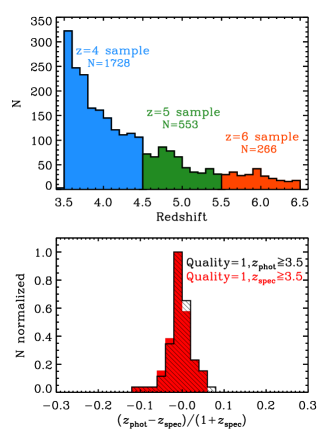
Figure 1 compares redshifts from the combined $P(z$) method with their highest-quality spectroscopic counterparts. The top panel exhibits a histogram of the number of objects used in our samples as a function of their photometric redshift. The bottom panel shows the ability of the photometric redshifts to recover known spectroscopic redshifts in the redshift range of this work.

Unless otherwise specified, we use the median absolute deviation (MAD) to compute the equivalent standard deviation, $\sigma_{\mathrm{MAD}}$, as the measure of scatter in given quantities (Beers et al., 1990), including the quoted scatter for redshift, stellar mass, and SFR. The $\sigma_{\mathrm{MAD}}$ is an analog for the 68% confidence, $\sigma$, if the error distribution were Gaussian and is therefore less sensitive to outliers (see Brammer et al., 2008). The MAD standard deviation in the photometric redshift accuracy ranges from $\sigma_{\mathrm{MAD}}/(1+z)$ = 0.016 at $z\sim 4$ to 0.028 at $z\sim 6$, indicating that these photometric redshifts reliably recover known spectroscopic redshifts at high redshift.

Even in the highest quality spectroscopic redshift sample, there is a non-zero chance that some objects will have a misidentified $z_{\text{spec}}$ due to a misinterpreted emission line or Lyman break (see discussion in Dahlen et al., 2013). So it is likely that some outliers are actually due to a misidentified $z_{\text{spec}}$ rather than a poorly fit $z_{\text{phot}}$ fit. The number of outliers where $|z_{\text{spec}}-z_{\text{phot}}|/(1+z_{\text{spec}})>$ 0.1 are 2, 1, and 1 for $z\sim$ 4, 5, and 6, respectively (only 5, 5, and 11% of each sample). For the remainder of this work we use the $z_{\text{phot}}$ catalog derived from the combined $P(z$) method, and substitute for high-quality ($z_{\text{qual}}=1$) spectroscopic redshifts when available.

2.3. Sample Selection

We selected objects according to their photometric-redshift ($3.5\leq z_{\text{phot}}\leq 6.5$). This redshift range was chosen to be close to the redshift range of the traditional $B$, $V$, and $i$ -drop samples. The lower redshift bound was chosen to avoid higher photometric redshift uncertainties, which may be due to a weaker Lyman break signal at $z<3.7$ (see Dahlen et al., 2013, their Fig. 11). Our samples have been cleaned from a total of 46 objects from X-Ray (Xue et al., 2011), IR (Donley et al., 2012), and radio (Padovani et al., 2011) detected AGN, as flagged by the Dahlen et al. (2013) photo-$z$ catalog.

Objects with a best-fit SED with $\chi^{2}>50$ are omitted from all samples. This cut removes objects with particularly poor fits, which comprise less than 4% of all objects. We interpret these objects as poor detections that do not well represent the data, and note that the removal of these objects do not impact the results of this work. The final sample includes 1728 objects with $3.5<z<4.5$, 553 objects with $4.5<z<5.5$, and 266 objects with $5.5<z<6.5$, as illustrated in Figure 1. We refer to these as the $z\sim 4$, 5, and 6 samples, respectively.

2.4. Galaxy Photometry from Models and Simulations

This work takes advantage of recent mock catalogs with synthetic photometry for galaxies from semi-analytic models (SAMs), as well as a semi-empirical dark matter and hydrodynamic simulation. We collectively refer to these as “the models”. The benefit of comparing our derived results against these model galaxies is that the models incorporate realistic star formation histories and galaxy physics. Here we use these models for two comparisons. First, in § 4.4 we derive stellar population parameters (SFRs and stellar masses) from the synthetic photometry for the model galaxies and compare to their “true” values as a test of our SED fitting procedures. Second, in § 5.2.2 we use our derived SFRs and stellar masses from the CANDELS samples to compare to the models and interpret the SFR–mass relation and its scatter.

2.4.1 SAMs of Somerville et al. and Lu et al.

This work uses the results of two SAMs that were specifically designed for the CANDELS GOODS-S field (Somerville et al., 2008, 2012; Lu et al., 2014, 2013, hereafter referred to as Somerville et al. and Lu et al. respectively), which we summarize here. Areas where the two SAMs differ are highlighted to emphasize the assumptions that lead to different SFR and stellar mass results. A more detailed comparison of the Somerville et al. and Lu et al. models can be found in Lu et al. (2013).

The mock catalogs produced by the SAMs are based on the Bolshoi $N$-body simulation (Klypin et al., 2011) for the same field-of-view size and geometry as the CANDELS GOODS-S field. The two SAMs are applied on the halo merger trees for halos in the mock catalogs. The models adopted a cosmology favored by WMAP7 data (Jarosik et al., 2011) and WMAP5 data (Dunkley et al., 2009; Komatsu et al., 2009) with $\Lambda$CDM cosmology. The mass resolution of the simulation is $1.35\times 10^{8}h^{-1}\hbox{M${}_{\odot}$}$, which allows the SAMs to track halos and subhalos with mass $\sim 2.70\times 10^{9}h^{-1}$ M_⊙.

The SAMs make explicit predictions for gas cooling rates, star formation, outflows induced by star formation feedback, and galaxy-galaxy mergers for every galaxy in the mock catalog. Both models assume that gas follows dark matter to collapse into a dark matter halo. When the gas collapses into the virial radius of the halo, it is heated by accretion shocks and forms a hot gaseous halo that cools radiatively. If the cooling timescale is longer than the halo dynamical time, both models follow the treatment that the halo gas cools gradually and settles on a central disk. The central disk of cold gas in both models is assumed to have an exponential radial profile, where stars form in regions where the surface density of the cold gas is higher than a threshold.

In the Somerville model, the SFR is predicted based on the cold gas surface density using the Schmidt–Kennicutt law (Kennicutt, 1998) explicitly. In the Lu et al. model, the star formation efficiency is assumed to be proportional to the total cold gas mass for star formation and inversely proportional to the dynamical time-scale of the disc, with an overall efficiency that matches observations (Lu et al., 2014).

Star formation feedback is assumed in both models, but the implementations are slightly different. Both models assume that the feedback reheats a fraction of the cold gas in the galaxy and a fraction of the reheated gas leaves the host halo in a strong outflow. However, the Lu et al. model allows a fraction of the kinetic energy of supernovae (SN) to drive an additional outflow to expel a fraction of hot halo gas. Nevertheless, the mass loading of the outflow in both models is assumed to be proportional to the SFR, and inversely proportional to a certain power of the halo maximum velocity. In the Somerville model, the mass-loading factor is assumed to be inversely proportional to the second power of the halo maximum velocity, mimicking the so-called “energy driven wind.” In the Lu et al. model, a much stronger power law of the halo circular velocity dependence is adopted. Both models assume a fraction of the ejected baryonic mass comes back to the halo as hot halo gas on a dynamical time-scale with different efficiencies.

The model parameters governing Star formation and feedback are tuned to match the local galaxy stellar mass function (Moustakas et al., 2013). The Lu et al. model is tuned using a Markov Chain Monte Carlo (MCMC) algorithm to find plausible models in the parameter space. The model precisely reproduces the local galaxy stellar mass function between $10^{9}$ and $10^{12}$ M_⊙, within the observational uncertainty. The Somerville model is further tuned based on a previously published model (Somerville et al., 2008) against the new data. In spite of different parameterizations adopted by the two models, they yield qualitatively similar predictions for the assembly histories of galaxy stellar mass and SFR over cosmic time.

2.4.2 Semi-empirical Matching of Observed Galaxies to Dark Matter Halos of Behroozi et al.

The semi-empirical model employed by (Behroozi et al., 2013b, BWC13 hereafter) uses a flexible fitting formula for the evolution of the stellar mass–halo mass relation with redshift, ($SM(M_{h},z)$; see BWC13 for further definition). This formula includes parameters for the characteristic stellar and halo masses, faint-end slope, massive-end shape, and scatter in stellar mass at fixed halo mass, as well as the redshift evolution of these quantities. Given halos from a dark matter simulation, each point in the $SM(M_{h},z)$ function parameter space represents an assignment of galaxy stellar masses to every halo at every redshift; the simulation and halo catalogs used by BWC13 are detailed by Klypin et al. (2011) and Behroozi et al. (2013c, d). The abundance of halos as a function of redshift can then be used to calculate the implied stellar mass function; the buildup of stellar mass over time in halos’ main progenitor branches can be used to calculate implied galaxy SFRs. BWC13 compares these predicted observables to published results from $z$ = 0 to $z$ = 8 and employs an MCMC algorithm to determine both the posterior distribution for $SM(M_{h},z)$ and the implied $SFR(M_{h},z)$. The resulting best-fits are consistent with all recent published observational results in this redshift range, including galaxy stellar mass functions, cosmic SFR, and sSFRs. Full details, including comparisons with other techniques for deriving the stellar mass–halo mass relation, are presented by BWC13.

2.4.3 Hydrodynamic Simulation of Davé et al.

This simulation was run with an extended version of the cosmological smooth particle hydrodynamic code Gadget-2 (Springel et al., 2005) described by Oppenheimer & Davé (2008). The simulation includes metal cooling and heating following Wiersma et al. (2009), star formation and a multi-phase interstellar medium model following Springel & Hernquist (2003), and galactic outflows assuming momentum-driven wind scalings which have been shown to be crucial for providing a reasonable match to a variety of intergalactic medium (IGM) and galaxy properties from $z\sim 0-4$ and beyond (see Davé et al., 2011b, a). The simulation employs a WMAP-7 concordant cosmology within a co-moving cube of length 48 Mpc/h per side with $2\times 384^{3}$ particles and 2.5 kpc/$h$ (co-moving) resolution. Mass growth in galaxies is resolved down to stellar masses of approximately $10^{9}\mathrm{M}_{\odot}$. See Davé et al. (2013) for a full description.

Table 1SED Fitting Parameters

Parameter	Quantity	Prior	Relevant Sections
Redshift	fixed	photometric redshifts, 3.5 $\leq z\leq$ 6.5	§ 2.2
Age	74	see equation C1 [$\log$, 10 Myr - $t_{\mathrm{max}}$]	§ 3, Appendix C
Metallicity	fixed	20% Z${}_{\sun}\ (Z=4\times 10^{-3})$	§ 3
Star formation history	fixed	100 Gyr (constant)	§ 3.1, Appendix A
$f_{\text{esc}}$	fixed	0 or 1	§ 3.2, Appendix B
$E(B-V)$	29	see equation C1 [Linear, 0.0 - 0.7]	§ 3.3, Appendix C
Attenuation prescription	fixed	starburst (Calzetti et al. 2000) or SMC (Pei et al. 1992)	§ 3.3, Appendix B
Stellar Mass	–	$\mathrm{M}_{\star}$$>0$, see equation C1	Appendix C

3. Stellar population synthesis fitting: Methods

This section describes the methods and assumptions used by our SED fitting procedure to derive physical quantities. This work uses a custom fitting procedure, using an updated version of the methods described by Papovich et al. (2001, 2006).

We utilize the Bruzual & Charlot (2011, private communication) SPS models, which are created with an updated version of the Bruzual & Charlot (2003) source code (BC03 hereafter) modified to accept rising star formation histories, $\Psi\sim\exp(+t/\tau)$, where $\tau$ is the $e$-folding timescale. We opt to use the libraries included with the BC03 models, as recent results have suggested the alternative 2007 libraries (similar TP-AGB contribution as Maraston (2005)) overestimate the contribution from TP-AGB stars in the near infrared (NIR), and the original BC03 version is likely to be more realistic (Kriek et al., 2010; Conroy & Gunn, 2010; Melbourne et al., 2012; Zibetti et al., 2013). Therefore, the remainder of this work uses the BC03 models. As mentioned above, we use a Salpeter (1955) IMF throughout which ranges in mass from 0.1–100 M_⊙.

Although we include the effects of H I absorption from IGM clouds along the line-of-sight to each galaxy (using the prescription of Meiksin (2006)), the true contribution of H I clouds to each galaxy will be highly stochastic. Therefore, we only include bands with wavelengths red-ward of the observed wavelength of Lyman-$\alpha$, given the galaxy redshift in our SED modeling. The redshift is fixed to the photometric redshift (or spectroscopic if available; see § 2.2), so fitting to bands blue-ward of Lyman-alpha offers no improvement in determining redshift.

Table 1 shows a list of the explored parameter space, as well as the degree to which each parameter is explored. The metallicity of all objects is fixed as 20% solar metallicity, partly due to a lack of confidence to accurately fit to this parameter given the degeneracies between fits to age and attenuation. The choice of 20% $Z_{\sun}$ is supported by recent work that suggests the metallicity of high-redshift ($z>2$) galaxies is low (Erb et al., 2006a; Maiolino et al., 2008; Erb et al., 2010; Finkelstein et al., 2011, 2012b; Song et al., 2014, see also Mitchell et al. (2013) for a discussion on the effects of metallicity in SED fitting).

Objects are fit to all available ages between 10 Myr and the age of the Universe at the redshift of the object, which is at maximum 1.8 Gyr at $z=3.5$. The age resolution of the BC03 models is quasi-logarithmic, with an average log difference in age steps of $\Delta t_{\text{age}}$/yr = 0.02 dex. We adopt a lower limit on the stellar population age of 10 Myr in order to avoid galaxies with ages younger than the minimum dynamical timescale of a galaxy at our specified redshifts (Papovich et al., 2001; Wuyts et al., 2009, 2011). In practice, we find that this minimum age has no impact on the fully marginalized parameter distributions.

Figure 2.— Four example galaxies from our sample with SED fits that do include nebular emission lines (blue curves) and do not include emission lines (black curves). Circles are the observed photometry and diamonds (squares) are the fluxes of the best-fit SED with (without) emission lines. The legends indicate the parameters of the best-fit model for both the case where the nebular emission is excluded and included, as labeled. All objects were fit assuming a constant star formation history and starburst-like dust attenuation. At certain redshifts (including the objects with $z=4.1$, 5.8, and 6.2), the IRAC 3.6 µm and 4.5 µm bandpasses may be enhanced by H$\beta$, [O III], or H$\alpha$ emission lines, as indicated. In contrast, the IRAC bands for the object with $z=5.1$ do not include of these prominent emission lines.

3.1. Star Formation History

One of the aims of this paper is to constrain the star formation history of the average population of galaxies at high redshift, $z>3.5$. Previous works have shown that broadband SED fitting offers no statistical preference between constant, rising, or declining star formation histories, even with broadband coverage spanning to the IR (Reddy et al., 2012). Furthermore, the star formation histories assumed in the templates can have non-negligible effects on the inferred SFRs, stellar masses, and ages (Lee et al., 2010). We addressed the shape of the star formation history as constrained by individual galaxies by running three separate fits using templates that assumed constant, declining and rising star formation history. The rising and declining star formation history templates (“$\tau$” models) included a suite of $e$-folding times. We ultimately found no obvious $\chi^{2}$ preference on the shape of the star formation history for individual galaxies.

Qualitatively, there has been some evidence to reject high-redshift star formation histories that decline with time. Previous studies have shown that high-redshift declining star formation histories would under-predict the sSFR at lower redshifts (Stark et al., 2009; González et al., 2010; Maraston et al., 2010). In addition, the instantaneous SFRs derived when assuming a declining star formation history will be under-produced by a factor of 5-10 as compared to direct estimates based off of UV-to-mid-infrared emission (Reddy et al., 2012). Other evidence against declining star formation histories comes independently from the SFR evolution of UV-luminous galaxies selected at fixed number density (Papovich et al., 2011). Finally, Pacifici et al. (2012) introduced a state-of-the-art SED fitting procedure with realistic, hierarchical mass-assembly histories and showed that declining $\tau$-model histories do not well represent galaxies even at ${z<2.}$

Although galaxies at $z>3$ likely have star formation histories that increase monotonically with time, we found it was impractical to use such models as the derived results are less physical. Our full justification for fitting individual galaxies with a constant star formation history is provided in Appendix A. Briefly, the BC03 stellar populations currently only allow for star formation histories that rise exponentially with time using simple parameterizations. At late times, such histories increase their SFR much faster than supported by observations. In Appendix A, we show that our modeling of synthetic photometry for galaxies from semi-analytic models recovers the most accurate stellar masses and SFRs when we adopt constant star formation histories. We interpret this as due to the fact that the SFRs in the models are approximately constant over the past $\sim$100 Myr (see, e.g., Finlator et al., 2006), and not consistent with exponentially increasing SFRs. Therefore, we fix the fitting templates to have a constant star formation history in our analysis of the CANDELS data for the remainder of this work. In a future work, we will explore possible improvements in parameters using models with star formation histories that increase as a power law in time ($\Psi\sim t^{\gamma}$).

3.2. Nebular Emission

This section presents our method of incorporating nebular emission. Nebular emission is important because many galaxies at high redshift are observed to have intense star formation and high equivalent widths (EW) from emission lines (Erb et al., 2010; van der Wel et al., 2011; Atek et al., 2011; Brammer et al., 2013). Such strong nebular emission is able to enhance broadband flux by up to a factor of $\sim 2-3$ in IRAC 3.6 and 4.5 µm bands (Shim et al., 2011). Previous studies have shown that the flux excess from high EW emission lines causes a systematic decrement in stellar mass and SFR inferred from SED fitting (Schaerer & de Barros, 2009, 2010; Ono et al., 2010; Finkelstein et al., 2011; de Barros et al., 2014; Reddy et al., 2012; Stark et al., 2013).

Figure 3.— Best-fit SED model fluxes with and without emission lines are shown as ratios for ISAAC K${}_{\text{s}}$, IRAC 3.6, and IRAC 4.5 bands as a function of redshift. Horizontal lines describe the redshift at which a strong emission is in the bandpass. The effect of adding emission lines is an increase to the model fluxes by as much as a factor of 2–3, especially in case of strong emission lines, such as [O III] or H$\alpha$.

3.2.1 Nebular Lines

The strength of a given emission line is dependent on the properties of both the gas cloud and the incident ionizing source. These properties include metallicity, ionization parameter, electron density, and number of ionizing photons. Inoue (2011) explored these parameters and the resulting strength of nebular emission in the regime of high-redshift galaxies by utilizing CLOUDY 08.00(Ferland et al., 1998), which we use in our incorporation method.

After modeling a wide parameter space of seven metallicities, five ionization parameters and five Hydrogen densities, Inoue (2011) reports 119 sets of metallicity-dependent emission line strength relative to H$\beta$. These line ratios, ranging from 1216 Å to 1 $\micron$, are in close agreement with empirical metal line ratios (Anders & Fritze-v. Alvensleben, 2003; Maiolino et al., 2008). We use the Inoue (2011) line ratios and include Paschen and Bracket series lines from Osterbrock & Ferland (2006) and Storey & Hummer (1995). Following Inoue (2011), we relate the H$\beta$ line luminosity to the incident number of Lyman-continuum photons as

$$\text{L}_{\text{H}\beta}\ =\ 4.78\times 10^{-13}\frac{1-f_{\mathrm{esc}}}{1+0.6f_{\text{esc}}}\text{N}_{\text{LyC}}\ [\text{ergs}^{-1}],$$ (1)

where $f_{\text{esc}}$ is the fraction of ionizing Lyman continuum (LyC) photons escaping the galaxy into the IGM and $\text{N}_{\text{LyC}}$ is the production rate of Hydrogen-ionizing photons (see also Osterbrock & Ferland, 2006; Ono et al., 2010). The number of ionizing Lyman-continuum photons, $N_{\mathrm{LyC}}$, depends on the age of the stellar population, and we take $N_{\mathrm{LyC}}$ from each BC03 SPS model for each age. It follows that $1-f_{\mathrm{esc}}$ is the fraction of LyC photons that ionize gas within the galaxy, which then produce the emission lines. The additional factor in the denominator of equation 1 comes from a ratio of recombination coefficients (see Inoue, 2011). Here, we equate the metallicity of the nebular gas to the metallicity of the SPS template (set as $Z=20\%\ Z_{\sun}$ for all models, see above). Following the results of Erb et al. (2006b), we attenuate both nebular and stellar emission in the same manner (see § 3.3 for details on attenuation).

The escape fraction has been measured to be low, i.e., $f_{\text{esc}}\approx 0$ at low redshift $z\sim$1 (see Malkan et al., 2003; Siana et al., 2007, 2010; Bridge et al., 2010). At $z\gtrsim 4$, the IGM imparts a large optical depth to ionizing photons, making it difficult to constrain $f_{\text{esc}}$. Nestor et al. (2011) used $z\sim 3$ Lyman Break Galaxies to study the high-redshift escape fraction, finding it to be consistent with $f_{\text{esc}}\approx 0.1$. Finkelstein et al. (2012a) concluded that if galaxies are the main contributors to reionization, then the escape fraction must be $f_{\text{esc}}<0.34$, or $f_{\text{esc}}<0.13$ (2$\sigma$) at $z\sim 6$ if the luminosity function extends to fainter galaxies than those observed, in order for the inferred ionization from galaxies to be consistent with the ionization background inferred from quasar spectra (Bolton & Haehnelt, 2007). In addition, Jones et al. (2013) reinforced this claim by finding the covering fraction of neutral hydrogen in $z\sim$4 galaxies to be lower by 25% compared to $z\sim$2-3. From these results, it seems reasonable to assume a low, but non-zero, escape fraction at high redshift.

Figure 4.— Four example galaxies with the largest differences in the SFR derived from the best-fit models using SMC and starburst attenuations. For each galaxy, the best-fit SEDs are shown for SMC (red) and starburst (black) attenuations. Circles are the observed photometry and squares (diamonds) are the fluxes of the best-fit SED with SMC (starburst) attenuation assumed. The legends indicate the derived properties when assuming each attenuation. All objects were fit assuming a constant star formation history with nebular emission lines. Objects may have similarly shaped SEDs, but the difference in $A_{V}$ drives the change in the inferred parameters. In all cases, the $\chi^{2}$ values are equal or exhibit no preference for the SMC or starburst attenuations.

Here we consider two limiting cases. The first has $f_{\mathrm{esc}}=1$, for which all LyC photons escape the galaxy, preventing the creation of nebular emission and reverting the spectrum to the output of the SPS model. The second case has $f_{\mathrm{esc}}=0$, for which all LyC photons are absorbed and their energy is converted into the nebular emission spectrum. These two cases span the range of possibilities and allow us to study the effects of nebular emission on the inferred physical parameters. Nevertheless, given current constraints of $f_{\mathrm{esc}}\sim 0.1$ (see above), we expect the $f_{\mathrm{esc}}=0$ case will provide a more physical model for galaxies in our sample.

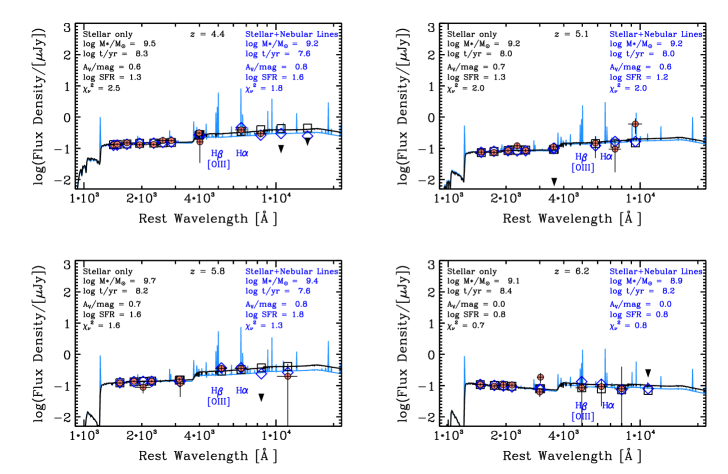
To illustrate the effect of nebular emission, Figure 2 displays four examples that include the best-fit SED models with and without nebular emission lines for galaxies. Depending on the redshift, emission from H$\alpha$ and/or [O III] will enhance the IRAC flux and can lead to highly different model-parameter values. The effect of nebular emission lines on the inferred stellar mass has a simple, qualitative explanation: the flux excess to the optical bands from nebular emission mimics a strong Balmer break that is typical for massive, older stellar populations. In this sense, when it is assumed that all of the observed broadband flux is produced by stars when much of it is produced by nebular emission, the inferred stellar mass will be over-estimated.

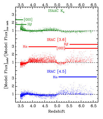
Similarly, Figure 3 illustrates how the specific emission lines ([O III], H$\beta$ , and H$\alpha$ ) affect the bandpass-averaged flux densities for the observed $K_{s}$ and IRAC [3.6] and [4.5] bands from the best-fit SED models. The inclusion of [O III], H$\alpha$, and H$\beta$ lines raise the flux of these bands by up to a factor of $\sim$2. In Appendix B, we explore how the effects of nebular emission lines change the best-fit stellar masses and SFRs. However, as we show below, these changes are largely mitigated using our Bayesian formalism.

3.2.2 Nebular Continuum

Evolutionary synthesis modeling suggests that nebular continuum emission can impact broadband photometry (Leitherer & Heckman, 1995; Mollá et al., 2009; Raiter et al., 2010). In addition, recent observational evidence has discovered the presence of strong nebular continuum in star-forming galaxies (Reines et al., 2010). The inverse Balmer and Paschen breaks (Balmer and Paschen “jumps”), may contribute additional flux red-ward of rest-frame optical wavelengths (Guseva et al., 2006). We currently omit these effects, as the strongest nebular continuum is present at wavelengths redder than rest-frame 8 µm (observed-frame $36-60~{}\micron$ for the redshift range investigated here), where the objects in this work are not well observed (see Zackrisson et al., 2008).

3.3. Dust Attenuation Prescriptions

Recent work has suggested that the typically assumed Calzetti et al. (2000) attenuation prescription for star-forming galaxies is not ubiquitous (Reddy et al., 2012; Oesch et al., 2013; Chevallard et al., 2013; Kriek & Conroy, 2013). The slope of the attenuation curve or presence of the UV dust bump at 2175  Å may be dependent on the galaxy type, geometry, metallicity, or inclination. However, galaxies at $z>4$ currently lack sufficient observations to quantify these effects, so some attenuation prescription must be assumed. This work aims to test the effects of changing the type of assumed attenuation in order to gauge its impact on our broadband SED fitting procedure. In this subsection, we describe the two different attenuation prescriptions used in this work: the Calzetti et al. (2000) attenuation prescription (“starburst”-like attenuation, hereafter), and the Pei (1992) attenuation prescription derived for the SMC (“SMC”-like attenuation, hereafter).

Figure 5.— Examples of the posterior cumulative probability densities on a given model parameter value, $\Theta$, for a galaxy with higher extinction (solid lines) and one with lower extinction (dashed lines), with $z_{\text{spec}}=4.142$ and 3.791, respectively. The posteriors in age are often broad, as it is the least constrained parameter. The posteriors in stellar mass are typically narrower. Throughout, we assign the medians of each parameter’s posterior (taken as the 50th percentile, shown as vertical lines) as the accepted value, with the 68% confidence range as the region that spans the 16th to 84th percentiles.

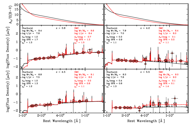
Figure 4 shows four example best-fit SEDs of objects that emphasize the difference in SFRs for best-fit models using the SMC and starburst dust prescriptions. The starburst attenuation has a much “grayer” wavelength dependence in the UV than the SMC-like attenuation. This means the SMC-like attenuation curve has a much stronger attenuation at rest-frame, far-UV wavelengths $\lambda\lesssim 1200$ Å, and a weaker attenuation across near-UV-to-near-infrared wavelengths $\lambda\gtrsim 1200$ Å, as shown in the top two panels of Figure 4. As stated above, bands shortward of Ly$\alpha$ are omitted in our procedure, so we do not fit where the difference between attenuation prescriptions is strongest.

We find no obvious preference in $\chi^{2}$ between the best-fit models for an SMC-like or starburst-like attenuation, and thus cannot as yet promote the use of one prescription over the other from this data set. However, we argue that the SMC-like attenuation could be invoked as a physical prior to reconcile the unphysical, extremely young stellar population ages that result from assuming a starburst-like attenuation. This method is preferred over, for example, increasing the minimum allowed age in the models (e.g., from $\geq$ 10 Myr to $\geq$ 60 Myr), which will not remove the preference of the fit to choose the youngest available age. A similar line of reasoning is used by Tilvi et al. (2013) to argue for SMC-like attenuation over starburst-like attenuation. Nevertheless, as we will show in § 4.3, in our Bayesian formalism these differences arising from changes in the dust prescription are mitigated, and the dust attenuation prescription has negligible impact on the results here.

4. A Bayesian approach to determine physical parameters

This section describes our method to measure the posterior probability density for each object and shows how the likelihoods for each stellar population parameter were determined during the SED fitting. For the remainder of this work, we consider the fully marginalized posterior probability density functions to derive constraints on physical quantities such as stellar population age, galaxy attenuation (i.e., dust extinction), SFR, and stellar mass.

Figure 6.— An example of the posterior, joint probability density between stellar mass and $M_{1500}$ for a single object (where here $M_{1500}$ is the observed value derived from the model parameters analogous in the way for the stellar mass, and is uncorrected for dust attenuation). Darker blue regions show higher probability density, and the yellow star denotes the accepted (median) values. The lower left to upper right covariance is typical for most objects and results from covariances between the extinction and age parameters. It is noteworthy that the scatter in $\mathrm{M}_{1500}$-$\mathrm{M}_{\star}$ for a single object is roughly orthogonal to the direction of the $\mathrm{M}_{1500}$-$\mathrm{M}_{\star}$ “main sequence” as derived from the full sample (see Fig. 10). Therefore, this scatter in $\mathrm{M}_{1500}$-$\mathrm{M}_{\star}$ likely contributes to the scatter in the SFR–mass sequence discussed later.

4.1. Probability Density Functions: Methods

Given a set of data for an individual galaxy which is a function of flux densities, D${(f_{\nu})}$, we derive the likelihood,

$$P(D|\Theta^{\prime})\ \propto\ \exp(-\chi^{2}/2)$$ (2)

where $\chi^{2}$ is measured between the data, $D$, and a model in the usual way for a given set of model stellar population parameters, ${\Theta^{\prime}=(\Theta\{t_{\text{age}},\tau,A_{\text{V}}\},\hbox{$\mathrm{M}_{\star}$})}$. Note that the likelihood in equation 2 is constructed based on linear fluxes. We then find the posterior probability density for any parameter given an observed set of data, $D$, and probability density using Bayes’ theorem (see also, Moustakas et al., 2013),

$$P(\Theta^{\prime}|D)=\ P(D|\Theta^{\prime})\times p(\Theta^{\prime})/\eta$$ (3)

where $\Theta^{\prime}$ represents the fitted parameters $\Theta$ and $\mathrm{M}_{\star}$, and $\eta$ is a constant such that $P(\Theta^{\prime}|D)$ will normalize to unity when integrated over all parameters (see Kauffmann et al., 2003). $p(\Theta^{\prime})$ represents the priors on the model parameters, and is described further in Appendix C. As described in § 3 and Table 1, we have adopted a prior (quasi-logarithmic) on the age from 10 Myr to the age of the Universe for a galaxy’s redshift, and we have adopted a prior (linear) that the attenuation is non-negative up to a maximum value. Further details on these priors and their effect on the fitting can be found in Appendix C.

Figure 7.— An example of the posterior joint probability between the SFR and stellar mass for one object. Darker blue regions show higher probability density and the yellow star denotes the accepted (median) values. The range in SFR is driven nearly entirely by the posterior probability density for attenuation, as described in the text (see equation 5). The covariance in SFR and stellar mass is mostly orthogonal to the “main sequence” as derived from the full sample (see Fig. 11), which implies that the scatter in the SFR–$\mathrm{M}_{\star}$ relation for individual galaxies translates to scatter in the SFR–$\mathrm{M}_{\star}$ relation for the galaxy population.

We then derive posterior probability densities on individual parameters such as $t_{\text{age}}$, $A_{\text{UV}}$, etc. For example, the posterior on the age can be written as,

$$P(t_{\text{age}}|D)\ =\int_{A_{\text{UV}},\tau}P(t_{\text{age}},A_{\text{UV}},\tau|D)\ dA_{\text{UV}}\ d\tau,$$ (4)

where the integration is a marginalization over “nuisance” parameters, dust attenuation, $A_{\text{UV}}$, and possible star formation histories/$e$-folding timescales, $\tau$.

The stellar mass must be treated differently because it is effectively a scale factor in the fitting process. In order to derive its posterior probability density we must integrate over all parameters, $P(\hbox{$\mathrm{M}_{\star}$}|$D$)\propto\int P($D$|\Theta^{\prime})*p(\Theta^{\prime})d\Theta.$ The mean and variance of the stellar mass can be computed as the first and second moments of the posterior. Similarly, the median stellar mass is defined as the value of $\mathrm{M}_{\star}$ such that the integral over the posterior from negative infinity to $\mathrm{M}_{\star}$ is equal to 50%, while the 68% confidence range can be calculated by integrating the posterior from the 16th to 84th percentiles.

4.2. Probability Density Functions: Results

We computed the posterior probability densities for all galaxies in our sample, including posteriors for the stellar mass, age, and attenuation, using the methods described above. Figure 5 shows examples of the cumulative posteriors on age, attenuation (or color excess, $E(B-V)$), and stellar mass for two galaxies in our sample: a relatively un-extincted and a relatively extincted galaxy. These objects are typical of those in the sample, where the posterior for age is typically broad, while that for the stellar mass is relatively tighter.

Figure 8.— The change in SFRs and stellar masses derived from the galaxy posteriors using different model assumptions. The top panels compare the SFRs and stellar masses derived using models that include and exclude nebular emission lines. The inclusion of nebular emission lines has minimal effect on the SFRs ($\lesssim 0.1$ dex), and the stellar masses have a slight decrease ($0.1-0.2$ dex) when nebular emission lines are included. The bottom panels compare SFRs and stellar masses derived using models with SMC-like and starburst-like dust attenuation. Here, varying the dust attenuation prescription has a negligible impact on the derived SFRs and stellar masses. These results can be directly compared to the results derived from best fits, which show much stronger differences in these quantities derived from these models (see Appendix B).

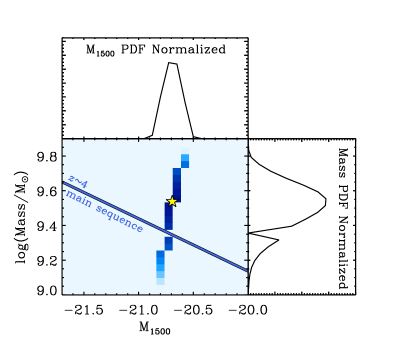
In our analysis below, we will consider the relation between stellar mass and UV magnitude, as well as stellar mass and SFR for our full galaxy sample. Here, we discuss the relation between stellar mass and these quantities for an individual object, as it is illustrative. Figure 6 shows a two-dimensional probability density function between stellar mass and UV absolute magnitude. Here we take the $\mathrm{M}_{1500}$ from the conditional posterior on age and attenuation (similar to way we derive the posterior for stellar mass given the model parameters and data). Figure 6 also shows the posterior for $\mathrm{M}_{1500}$ and stellar mass individually.

There is a weak covariance between $\mathrm{M}_{1500}$ and $\mathrm{M}_{\star}$, which results from the degeneracy in dust attenuation and age. A galaxy with a redder rest-frame UV continuum has near equal likelihood to a model with an older, less extincted stellar population as to a model with younger, higher extinction. The two models produce a joint posterior that is anticorrelated between $\mathrm{M}_{1500}$ and stellar mass. The figure also shows the “main sequence” of the $\mathrm{M}_{1500}$–$\mathrm{M}_{\star}$ relation as derived from the full sample (see Fig. 10). The joint posterior is approximately orthogonal to the main sequence, which implies that the likelihood scatter in each galaxy’s $\mathrm{M}_{1500}$–$\mathrm{M}_{\star}$ plane will lead directly to scatter in the main sequence of the sample. We return to this point in the discussion of the SFR-$\mathrm{M}_{\star}$ relation below.

Figure 9.— Tests of the derived SFRs and stellar masses from the posteriors of our SED fitting to synthetic photometry of mock catalogs from the SAM of Somerville et al. The top panels show the log difference of measured-to-true SFRs. The derived SFRs show a weak trend in that our fits overestimate the SFRs of low-SFR objects and underestimate the SFRs of high-SFR objects. The middle panels show the ratio of the measured-to-true stellar masses. The scatter in the derived stellar masses from their true values likely arises from our simple prescription for the star formation histories (similar offsets are observed by Lee et al. (2010)). The bottom panels show that our derived SFRs and stellar masses recover the SFR–mass relation in the models, though with a more shallow slope. The legend to the lower right indicates the slope, zero point, and scatter of the SFR–mass relation for the SAMs and those recovered using best-fit values or our preferred marginalized values. The main point of the figure is that the bayesian method does better at recovering both the SFRs and stellar masses and the SF main sequence.

We derive the SFR from the model parameters in the following manner. We first determine the rest-frame UV luminosity at 1500 Å. At these redshifts, a large sample of detections red-ward of the rest-frame optical are unavailable, which can cause age and attenuation inferred from SED fitting to be degenerate quantities. These degeneracies can bias the $\mathrm{M}_{1500}$ inferred from the model parameters, especially if limited to best-fit values (see the discussion above and Appendix B). For this reason, we choose the closest observed band to rest-frame 1500 Å as a more observationally motivated value of $\mathrm{M}_{1500}$ because the broad-band photometry well samples the rest-frame UV portion of the SED. Galaxies have relatively blue rest-frame UV colors, so any corrections between the band closest to 1500 Å and the interpolated magnitude at 1500 Å are small (in the “extreme” examples of Figure 4 the differences are $<$ 0.1 mag). Furthermore, our tests show that none of our conclusions depend strongly on the manner we use to obtain $\mathrm{M}_{1500}$.

The 1500 Å luminosity is corrected for dust attenuation using the median from the posterior of the attenuation at 1500 Å, or $A_{\text{UV}}$. The dust-corrected UV luminosity is converted to the SFR${}_{\text{UV}}$ using the ratio $\kappa(t,\tau)=$ SFR${}_{\text{UV}}$$/L_{1500}$. This is similar to the conversion given by Kennicutt (1998), but we account for variations in SFR${}_{\text{UV}}$$/L_{1500}$ owing to the age ($t$) and star formation history ($\tau$) of the stellar population (see, Reddy et al., 2012). For each object, we use the median stellar population age from the posterior to calculate SFR${}_{\text{UV}}$$/L_{1500}$. However, we note that because most of these median ages from posteriors are $>$100 Myr for the galaxies in our sample and we have assumed constant star formation histories, in most cases $\kappa(t,\tau)$ is very similar to that of Kennicutt (1998).

We summarize the derivation of our SFR${}_{\text{UV}}$ mathematically as follows.

$$\mathrm{SFR}_{\text{UV}}=f_{\text{CB}}\cdot\frac{4\pi D_{L}^{2}}{1+z}\cdot 10^{0.4\ A_{\text{UV}}}\cdot\kappa(t,\tau)$$ (5)

where $f_{\text{CB}}$ is the flux of the closest band to rest-frame 1500 Å, $D_{L}$ is the luminosity distance, $A_{\text{UV}}$ is the median, marginalized attenuation at 1500 Å, and $\kappa$ is the modified Kennicutt (1998) conversion that depends on age ($t_{\mathrm{age}}$) and star formation history ($\tau$).

The differences between the SFRs derived using equation 5 and other common methods are described in Appendix B. In summary, methods that derive the SFR using the best-fit or direct UV luminosity slope exhibit higher scatter when compared to the marginalized SFR method from this work. This scatter stems from degeneracies between the young, dusty and old, dust-free solutions of a given SED, and photometric uncertainties (which affect the accuracy of measuring the UV spectral slope). We find the results of our method more robust as it reproduces SFRs from SAMs (see § 4.4), and our method is relatively unaffected by model variations such as extinction prescription and/or nebular emission lines.

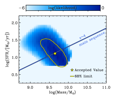
Figure 7 shows the SFR–stellar mass joint posterior for one object from our sample. As with the $\mathrm{M}_{1500}$–$\mathrm{M}_{\star}$ example, the covariance is roughly orthogonal to the star formation main-sequence, but there is more scatter because of the range in dust attenuation (and, to a lesser extent, the stellar population age). The errors on the measured (extrinsic, or attenuated) $\mathrm{M}_{1500}$ are relatively small as they stem from photometric errors only, whereas the SFR depends on the UV luminosity corrected by the UV extinction, $A_{\mathrm{UV}}$.

SED models with higher $A_{\mathrm{UV}}$ have higher stellar-mass–to–light ratios (and therefore higher stellar masses at fixed UV luminosity). This induces some correlation in the SFR–stellar mass plane for each object. However, the covariance is mostly orthogonal to the expected direction of the SFR–stellar mass correlation, which implies that it contributes mostly to the scatter of the SFR–stellar mass relation and less to the correlation itself. In our analysis we take this covariance into account using Monte Carlo simulations (see § 5.2.1).

4.3. Impact of SED Fitting Assumptions on Marginalized Values

Here we discuss our SED model assumptions and their impact on derived quantities such as SFR and stellar mass using our Bayesian method. In Appendix B, we show that these model choices have a significantly stronger impact on best-fit results, while the results using medians derived from posteriors are relatively unaffected.

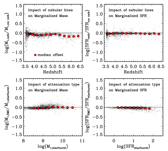
The panels of Figure 8 show that the SFRs and stellar masses derived from the posteriors for the galaxies in our sample are rather insensitive to the choice of dust-attenuation prescription or the presence/exclusion of nebular emission (where we compare the results with $f_{\text{esc}}$=0 or 1). In general, varying the assumed dust attenuation prescription has a negligible impact on the derived SFRs and stellar masses (differences are $<$0.1 dex over the redshift range of our sample). Similarly, including emission lines has minimal effect on the SFRs ($\lesssim 0.1$ dex).

There is some evidence that the stellar masses are reduced slightly when the models include nebular emission lines. This is in the same direction but weaker in magnitude as seen in comparisons of the best-fit models (e.g., see Appendix B). However, the effect is only a slight decrease of $<0.25$ dex, and is typically less than the measurement errors on mass derived from the posteriors. Therefore, the inclusion of nebular emission does not strongly impact the SFRs or stellar masses. For this reason, we have neglected exploring nebular emission over the full range of $f_{\mathrm{esc}}$ values in our analysis, and instead report results assuming $f_{\mathrm{esc}}=0$ (all ionizing radiation is absorbed and produces emission lines).

The results from Figure 8 can be directly compared to the results derived from best-fits, which show stronger differences in these quantities when switching between the above model assumptions (see Appendix B). In contrast to using best-fit values, the Bayesian method uses the likelihood of all the models, and so even if there is a “highest likelihood” solution of low age, there are many good solutions with larger ages, and when marginalized, the latter dominate the posterior.

Figure 10.— The closest band to rest-frame UV magnitude ($\mathrm{M}_{1500}$) versus stellar mass. Darker-shaded regions indicate a higher number of individual objects in bins of stellar mass and $\mathrm{M}_{1500}$. Yellow circles are the medians of stellar mass in a given $\mathrm{M}_{1500}$ bin and error bars are the $\sigma_{\mathrm{MAD}}$ confidence range (analogous to the 68% confidence, $\sigma$, if the error distribution were Gaussian, see § 2.2). Red triangles, white triangles, and white diamonds are medians from Lee et al. (2011), Lee et al. (2012), and Stark et al. (2013) respectively. Bottom right: For reference, this cartoon shows the strength and direction of galaxy evolution over 590 Myr from $z\sim 6$ to $z\sim 4$ under an assumed star formation history. This plot implies that there is a weak relation between UV magnitude and stellar mass in place up to $z\sim 6$ with significant scatter, and that rising star formation histories offer a simple explanation of how galaxies may evolve along this relation.

4.4. Tests of Derived SFR and Stellar Masses using Semi-Analytic Models

We tested the ability of our SED fitting procedure to reproduce accurately the SFRs and stellar masses in mock galaxy catalogs. We used synthetic galaxy photometry in the CANDELS bandpasses derived from the Somerville et al. SAM discussed in § 2.4.1. The advantage of using synthetic catalogs from a SAM is that the models include realistic (and complex) star formation histories, as well as more sophisticated treatments of extinction (e.g., Charlot & Fall, 2000). Therefore, the mock catalog from the SAM acts as a realistic observation where many of the model parameters (star formation history, extinction prescription) are known, and are distinct from the simpler models used in SED fitting to fit to the galaxy photometry. Comparing to the SAMs therefore provides a powerful test of our method to recover physical stellar population parameters, even when the physical details are unknown, such as the case of our observed galaxies. A similar but more comprehensive study was conducted among many CANDELS team members which compared the estimated and expected parameters from galaxies measured using SED fits (see Mobasher et al., in prep.).

Table 2M₁₅₀₀ – Stellar Mass Relation Median Values

$z\sim 4$

$\mathrm{M}_{1500}$	-21.5	-21.0	-20.5	-20.0	-19.5	-19.0	-18.5
$\log$(Median Mass/M⊙)	9.61	9.50	9.21	9.13	8.96	8.81	8.75
$\sigma_{\text{MAD}}$	0.39	0.57	0.47	0.51	0.56	0.53	0.57

$z\sim 5$

$\mathrm{M}_{1500}$	-21.5	-21.0	-20.5	-20.0	-19.5	-19.0	-18.5
$\log$(Median Mass/M⊙)	9.67	9.44	9.18	9.07	8.88	8.91	8.76
$\sigma_{\text{MAD}}$	0.35	0.43	0.52	0.52	0.50	0.66	0.53

$z\sim 6$

$\mathrm{M}_{1500}$	-21.5	-21.0	-20.5	-20.0	-19.5	-19.0	-18.5
$\log$(Median Mass/M⊙)	9.34	9.23	9.21	9.14	8.90	8.77	—
$\sigma_{\text{MAD}}$	0.44	0.38	0.41	0.38	0.38	0.47	—

The mock catalog from the SAM was filtered to a sample of 6000 simulated galaxies, evenly distributed across the mass and redshift range of our CANDELS sample. We took the synthetic photometry from the models and randomly perturbed them according to a Gaussian error distribution with a similar $\sigma$ as the CANDELS data at a given band and magnitude. This process accounts for any systematic errors in creating the mock catalogs, and we process these fluxes the same way we process the data, even when fluxes are perturbed to negative values. These fluxes were used as input to the same SED-fitting procedure we applied to the real CANDELS samples. The masses and SFRs in the SAM were scaled to a Salpeter IMF, to match our procedure. We also fit to templates that exclude the effects of nebular emission (using $f_{\mathrm{esc}}=1$) because the SAMs also exclude nebular effects. For the test here, we show only the case where we fix the star formation history to be constant. Our tests (discussed in Appendix A) show that we recover the most accurate SFRs and stellar masses using constant star formation histories. Appendix A discusses how including additional star formation histories affects the SFRs and stellar masses.

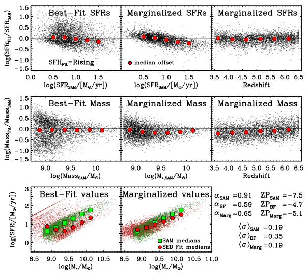
Figure 9 compares the “true” stellar masses and SFRs from the SAM with those derived from using either the “best-fit” values or our method of taking the median, marginalized value from the posterior. This figure shows that taking advantage of the whole posterior with marginalized values produces less scatter in the recovering the “true” SAM values. This is because the maximum likelihood can be more sensitive to template assumptions than the median posterior values, as shown in Figure 8 and discussed in Appendix B. We note that there is a weak systematic where the fits slightly overestimate objects with low SFRs and slightly underestimate objects with high SFRs. The effect is mild, ranging by $\pm 0.25$ dex. This systematic could be due to differences in the extinction prescription and assumed star formation history between models used in the fit and those in the SAM.

The bottom panel of Figure 9 shows that the offsets in stellar mass and SFRs conspire to reproduce the accurate SFR–mass relation as expected from the SAMs. The parameters derived from our fits better reproduce the zero point, scatter, and slope of the relation than when using best-fit values. We also find no appreciable difference in the ability to recover the SFR–stellar mass relation across redshift. Our ability to test the success of our procedure, however, is limited to the maximal level of stochasticity in the star formation histories of the SAMs and we have not tested our procedure to observe its sensitivity to very bursty star formation histories. Nevertheless, these tests give us confidence that even in the presence of realistic photometric errors, we are able to derive a SFR–stellar mass relation from high-redshift galaxies in the CANDELS data that reproduces the intrinsic relation within these $\sim$ 0.25 dex uncertainties in SFR or stellar mass.

Figure 11.— The SFR–stellar mass relation for the CANDELS galaxy samples. The darker-shaded regions indicate a higher number of individual objects in bins of stellar mass and SFR. Yellow circles are medians in bins of mass and yellow error bars are their $\sigma_{\mathrm{MAD}}$ confidence range (see Table 3). The median SFR of a wider, high-mass bin is also shown by the dashed black circle. The white hatched regions mark the limit above which completeness effects become negligible. We measure a slope of $\sim$0.6 (see Table 4), with no evidence for evolution over the redshift range $z\sim$6 to 4. The purple error bars show the 68% range of errors from the Monte Carlo simulations described in § 5.2.1.

Table 3SFR – Stellar Mass Relation Median Values

$z\sim 4$

$\log$($\mathrm{M}_{\star}$/M⊙)	9.00	9.25	9.50	9.75	10.00	10.25	$>$ 10.375
$\log$(Median SFR/M⊙ yr-1)	0.71	0.90	1.01	1.04	1.35	1.51	1.87
$\sigma_{\text{MAD}}$	0.36	0.41	0.35	0.24	0.27	0.25	0.24
Monte Carlo $\sigma$	0.26	0.33	0.31	0.31	0.27	0.29	—

$z\sim 5$

$\log$($\mathrm{M}_{\star}$/M⊙)	9.00	9.25	9.50	9.75	10.00	10.25	$>$ 10.375
$\log$(Median SFR/M⊙ yr-1)	0.88	1.04	1.12	1.23	1.46	1.62	1.85
$\sigma_{\text{MAD}}$	0.42	0.38	0.41	0.43	0.31	0.37	0.33
Monte Carlo $\sigma$	0.25	0.33	0.36	0.28	0.27	0.25	—

$z\sim 6$

$\log$($\mathrm{M}_{\star}$/M⊙)	9.00	9.25	9.50	9.75	10.00	$>$ 10.125	—–
$\log$(Median SFR/M⊙ yr-1)	0.92	1.07	1.27	1.40	1.47	1.79	—–
$\sigma_{\text{MAD}}$	0.19	0.21	0.35	0.26	0.07	0.35	—–
Monte Carlo $\sigma$	0.43	0.34	0.32	0.36	0.27	—–	—–

5. Evolution of SFR and Stellar Mass at $3.5<{z}<6.5$

This section describes the relations between the observed rest-frame UV magnitude, $\mathrm{M}_{1500}$, and stellar mass, and the SFR and stellar mass of galaxies in our CANDELS sample from $z$ = 3.5 to 6.5. All SFRs and stellar masses are derived from the posteriors from the SED fits.

5.1. $M_{1500}$–Stellar Mass Relation

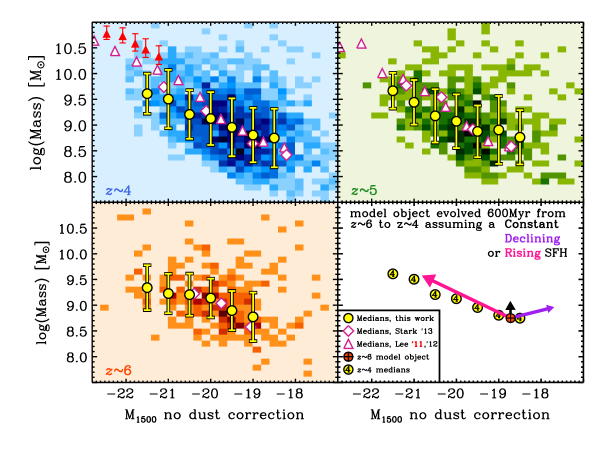
The panels of Figure 10 show the relation between the observed magnitude of the band closest to 1500 Å at the redshift of the galaxy (the rest-frame UV magnitude) and stellar mass at each redshift as two-dimensional histograms for our CANDELS sample. The median and $\sigma$ of stellar mass in each bin of $\mathrm{M}_{1500}$ are given in Table 2. Here we show the observed UV absolute magnitude with no dust corrections in order to easily compare against previous studies (Stark et al., 2009, 2013; Lee et al., 2011, 2012). As discussed above, quantities used in this figure are median stellar masses derived from the marginalized PDF of each object (see § 4 for details).

We find a correlation between UV absolute magnitude and stellar mass, though this relation retains significant scatter. Recent evidence has suggested a relation with significant scatter between $\mathrm{M}_{1500}$ and stellar mass at high redshift, $z\gtrsim 2$ (Reddy et al., 2006; Daddi et al., 2007; Stark et al., 2009; González et al., 2011; Reddy et al., 2012; Schaerer et al., 2013; Stark et al., 2013). The $\mathrm{M}_{1500}$–stellar mass trend in this work is weaker than the literature because we use an $H_{160}$-band selected catalog, which is closer to stellar mass than optically selected samples, as were used in the previous works listed above. This means that at fixed UV luminosity (or SFR) we are less sensitive to blue sources, which have higher mass-to-light ratios. Therefore, below our limiting stellar mass ($10^{9}$/M_⊙) we may be missing the bluer sources, as seen in Figure 10. At bright magnitudes (SFRs) our results agree with previous studies (that usually used $z_{850}$-band selected catalogs). It is at fainter magnitudes where our sources have fewer low-mass objects compared to the literature. Our results are also consistent with an independent analysis of the CANDELS catalogs, which used the same $H_{160}$-band selection (Duncan et al., 2014).

Regardless of the median relation, we consider the large scatter in $\mathrm{M}_{1500}$ at fixed stellar mass to mean one or both of the following. First, it could mean gas accretion is low such that galaxies undergo recurrent and stochastic star formation that leads to a range of $\mathrm{M}_{1500}$ at a fixed stellar mass (Lee et al., 2006, 2011). Second, galaxies at a fixed redshift and fixed stellar mass could exhibit a range of $A_{\text{UV}}$ attenuations. In the second scenario, the observed scatter in the plane of $\mathrm{M}_{1500}$–$\mathrm{M}_{\star}$ would be largely diminished once we apply corrections for dust attenuation. As discussed in the next subsection, the simulations favor the latter scenario.

The bottom right panel of Figure 10 illustrates an evolutionary cartoon depicting a model z$\sim$ 6 object of a given mass that is evolved forward $\approx$ 600 Myr to $z\sim 4$. This is done by assuming an initial stellar mass (10⁸ M_☉), age ($\sim$ 500 Myr, the average marginalized age of our entire sample), and zero dust ($A_{\text{UV}}$= 0). The strength and direction of three different star formation histories with the Bruzual & Charlot (2003) SPS code are shown: a constant SFR, a declining SFR (where $\Psi\sim\exp(-t/\tau)$, with $\tau=$ 1 Gyr), or a rising SFR (where $\Psi\sim t^{\gamma}$ using our results derived below from § 6.2). As illustrated in Figure 10, only a rising star formation history naturally evolves galaxies along the median relation between stellar mass and $\mathrm{M}_{1500}$. Though this simple explanation does well to explain the UV-faint to UV-bright evolution, it offers little insight to the fate of the UV-bright galaxies at later epochs. It remains to be seen if some population of massive, UV-bright galaxies at $z\sim 6$ quench their SFR such that we are missing a population of massive UV-faint galaxies at $z\sim 4$.

5.2. SFR–Stellar Mass Relation

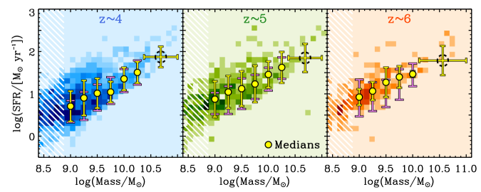
Figure 11 shows the relation between the (dust-corrected) SFR and the stellar mass, where both parameters are derived from the fully marginalized probability density functions. Table 3 shows the median and $\sigma$ scatter of $\log$ SFR in bins of stellar mass from Figure 11. We measure a tight SFR–stellar mass relation (a “main sequence”) for galaxies with $\log M_{\star}/$M_⊙$>9$, the mass completeness limit (e.g., Duncan et al., 2014). We explore how our SED fitting process could contribute to the correlation between SFR and stellar mass in Appendix C. This main-sequence in the SFR–mass relation has received much attention in the literature, and its existence implies that stellar mass and star formation both scale with the star formation history (Stark et al., 2009; González et al., 2010; Papovich et al., 2011). If true, then it follows that the gas accretion onto dark-matter halos at higher redshift is smooth when averaged over large timescales and stellar mass growth at high redshift is not driven by mergers (Cattaneo et al., 2011; Finlator et al., 2011). Our results support this picture.

We fit a linear relation to the SFR–stellar mass relation as

$$\log(\mathrm{SFR}/\mathrm{M}_{\odot}\ \mathrm{yr}^{-1})=a\ \log(M_{\star}/\mathrm{M}_{\odot})+b$$ (6)

where $a$ is the slope of the relation and $b$ is a zero point. The fitted values for $a$ and $b$ are given in Table 4. We also show the fitted values for $b$ when the slope is fixed to be $a=1$, since the slope and intercept are often degenerate. We find that the slope and normalization in the SFR–mass relation shows no indication for evolution, with slopes of $a$ $=0.54\pm\ 0.16$ at $z\sim 6$ and $0.70\pm\ 0.21$ at $z\sim 4$. Furthermore, the scatter in SFR at fixed stellar mass shows no evidence for evolution, with a range of $\sigma(\log\mathrm{SFR/\mathrm{M}_{\odot}\mathrm{yr}^{-1}})=0.2-0.4$ dex from the median.

Figure 12.— The SFR–stellar mass relation predicted from the models. Each set of lines or shaded swatch shows the $\pm\sigma$-range of galaxies from each model as given in the inset. The yellow points and errors bars show the measured relation for the CANDELS samples and are identical to the points in Figure 11. The zero point, scatter and slope of the SFR–stellar mass relation from the models is consistent with the measured values over this redshift range.

Table 4SFR–Stellar Mass Best-Fit Parameters

$z\sim 4$

	Slope $a$	Zero Point $b$	$b$ when $a\equiv 1$	$\langle\sigma_{\mathrm{MAD}}\rangle$	$\chi^{2}$
This work	0.70 $\pm$ 0.21	-5.7 $\pm$ 2.1	-8.64 $\pm$ 0.11	0.35 (0.31)	0.38
Somerville et al.	1.1 $\pm$ 0.13	-9.0 $\pm$ 1.3	-8.47 $\pm$ 0.05	0.18	0.06
Behroozi et al. 2013	1.1 $\pm$ 0.07	-9.2 $\pm$ 0.7	-8.47 $\pm$ 0.03	0.10	0.17
Lu et al.	0.80 $\pm$ 0.11	-6.5 $\pm$ 1.1	-8.45 $\pm$ 0.04	0.14	0.44
Dave et al. 2013	0.80 $\pm$ 0.05	-6.8 $\pm$ 0.6	-8.95 $\pm$ 0.03	0.16	2.1

$z\sim$5

	Slope $a$	Zero Point $b$	$b$ when $a\equiv 1$	$\langle\sigma_{\mathrm{MAD}}\rangle$	$\chi^{2}$
This work	0.59 $\pm$ 0.26	-4.4 $\pm$ 2.6	-8.49 $\pm$ 0.14	0.41 (0.29)d	0.05
Somerville et al.	1.0 $\pm$ 0.09	-8.6 $\pm$ 0.9	-8.29 $\pm$ 0.03	0.13	0.07
Behroozi et al. 2013	1.0 $\pm$ 0.05	-8.6 $\pm$ 0.5	-8.32 $\pm$ 0.02	0.07	0.35
Lu et al.	0.79 $\pm$ 0.07	-6.3 $\pm$ 0.7	-8.29 $\pm$ 0.02	0.10	0.78
Dave et al. 2013	0.80 $\pm$ 0.07	-6.7 $\pm$ 0.7	-8.72 $\pm$ 0.02	0.15	1.5

$z\sim$6

	Slope $a$	Zero Point $b$	$b$ fwhen $a\equiv 1$	$\langle\sigma_{\mathrm{MAD}}\rangle$	$\chi^{2}$
This work	0.54 $\pm$ 0.16	-3.9 $\pm$ 1.6	-8.45 $\pm$ 0.06	0.21 (0.34)d	0.10
Somerville et al.	1.0 $\pm$ 0.06	-8.5 $\pm$ 0.6	-8.16 $\pm$ 0.02	0.10	0.47
Behroozi et al. 2013	0.96 $\pm$ 0.05	-7.8 $\pm$ 0.5	-8.21 $\pm$ 0.02	0.07	0.81
Lu et al.	0.77 $\pm$ 0.07	-6.0 $\pm$ 0.7	-8.15 $\pm$ 0.02	0.10	1.3
Dave et al. 2013	1.1 $\pm$ 0.10	-9.6 $\pm$ 0.9	-8.29 $\pm$ 0.03	0.15	6.7

We must consider the possibility that the scatter in SFR at fixed mass is higher, and we are simply missing galaxies with low SFR due to incompleteness. We consider this unlikely because even if star formation ceased in some fraction of the galaxies, the galaxies would require $0.5-1$ Gyr to have their SFR drop below a detectable threshold in the WFC3 IR data. These timescales are comparable to the period of time spanned by our subsamples (i.e. the lookback time between $z=4.5$ and 3.5 is only 480 Myr), so it seems unlikely galaxies would “instantly” move from the observed SFR–mass sequence to undetectable values. For example, if such low-SFR objects existed at $z=4$ their progenitors should be seen at $z=5$ and 6 as they are fading, inducing a larger scatter in SFR–stellar mass. This work finds no evidence for such a population in our sample. Parenthetically, we note that some studies report evidence for massive, $\log M_{\star}/\mathrm{M}_{\odot}>10.6$ dex, quiescent galaxies at $z\sim 3-4$, but this population lies at stellar masses above those in our sample (Straatman et al., 2014; Muzzin et al., 2013; Spitler et al., 2014).

We note that our SFR–stellar mass relation is tighter than our $\mathrm{M}_{1500}$–stellar mass relation (Fig. 10), and we find that this can be explained by a correlation between stellar mass and our derived dust attenuation (there is no correlation between derived attenuation and $\mathrm{M}_{1500}$). For example, objects at masses of $10^{8.5}$, $10^{9.5}$, and $10^{10.5}$ M_⊙ have median marginalized $E(B-V)$ values of 0.05$\pm$0.03, 0.13$\pm$0.07, and 0.32$\pm$0.18 respectively. This relation accounts for the differences in the scatter seen in Figures 10 and 11.

5.2.1 Constraints on the Intrinsic Scatter in the SFR–Mass Relation

Before comparing against models, it is necessary to understand how much of the scatter in the SFR–mass relation is intrinsic to the galaxy population and how much is a result of observational errors in SFR and stellar mass. To a simple approximation, the observed scatter (yellow in Fig. 11) is a combination of the intrinsic (true) scatter and the measurement errors added in quadrature,

$$\sigma_{\mathrm{observed}}=(\sigma_{\mathrm{intrinsic}}^{2}+\sigma_{\mathrm{errors}}^{2})^{1/2}.$$ (7)

The SFR–mass joint probability density is broad, with covariance between the SFR and stellar mass (e.g., Fig. 7). Because we calculate the posterior probability density functions for both the stellar mass and SFR for galaxies in our samples, we are able to estimate how correlations in these parameters contribute to the scatter and slope of the SFR and stellar mass relation. Here we use a Monte Carlo simulation to estimate $\sigma_{\mathrm{errors}}$, and to determine how these errors affect the slope of the SFR–stellar mass relation.

We set up the Monte Carlo as follows. As discussed above, the SFR and stellar mass posteriors are covariant because both involve the dust attenuation, $A_{\mathrm{UV}}$, where models with higher $A_{\mathrm{UV}}$ have higher SFR from dust corrections, and higher mass-to-light ratios, which produce higher stellar masses. For each galaxy in each subsample at $z=4$, 5 and 6, we randomly sample the galaxy’s posterior density function of $A_{\text{UV}}$ to find a new UV attenuation, $A_{\text{UV},i}$. We then compute the conditional posterior for the stellar mass, $P($$\mathrm{M}_{\star}$$|A_{UV,i})$. Next, we derive the SFR from equation 5 and the medians of SFR in bins of stellar mass are re-calculated. This process is repeated $10^{4}$ times for each galaxy to generate $10^{4}$ new realizations of our galaxy sample. We then calculate at each stellar mass the median SFR and compute the $\sigma_{\mathrm{MAD}}$ from the distribution of medians. The scatter in $\log$ SFR from this Monte Carlo is shown in Figure 11 and Table 3.

The $\sigma_{\mathrm{MAD}}$ scatter in the SFR from the Monte Carlo simulations is comparable to the observed SFR scatter, $\sigma_{\mathrm{observed}}$, in most bins of mass and redshift. The scatter in the SFRs at fixed stellar mass from the Monte Carlo are shown in Figure 11 and given in Table 3. We make the approximation that $\sigma_{\mathrm{errors}}=\sigma_{\mathrm{MAD}}$ from the Monte Carlo. We subtract these in quadrature from the observed SFR scatter to estimate the intrinsic scatter in SFR at fixed mass using equation 7. We find that the average intrinsic scatter in SFR across the mass bins to be $\sigma=0.26\pm 0.04,0.23\pm 0.10,$ and $0.34\pm 0.11$ at $z\sim 4,5,$ and 6, respectively. In some instances, the measurement errors from the Monte Carlo accounts for more scatter than the observed scatter, in which case there is no meaningful constraint on the intrinsic scatter. In this case, we take the Monte Carlo measurement scatter alone as a conservative limit on the intrinsic scatter (as some of the errors on the derived quantities must arise from the intrinsic scatter). This has implications for the gas accretion rate that we discuss below in § 6.1.

The above test ignores the effects of our photometric redshift uncertainties since redshift is a fixed parameter during the fitting process. We constructed the following test to determine the effects of redshift uncertainties on SFR and stellar mass. We randomly selected 100 objects from each redshift sample and performed a Monte Carlo on their redshift uncertainty. In the Monte Carlo, each object’s redshift was re-assigned according to a Gaussian error distribution with a sigma equal to the object’s 68% photometric redshift uncertainty. Then, we derived the stellar masses and SFRs in the same manner as with the data, fixing the redshifts to be the new redshift values. We calculated the medians in the SFR–stellar mass relation, as in as in Figure 11, for each of $10^{4}$ realizations of this process. Finally, we found the median and $\sigma$ of SFR in each stellar mass bin from the distribution of SFR medians that each Monte Carlo realization produced.

Redshift errors produce a higher median $\log$ SFR of $<$0.1 dex per stellar mass bin, and the redshift errors can contribute as much as $\sim$0.1 dex to the scatter in every stellar mass bin (usually it is much smaller, contributing $<$0.03 dex for 50% of the stellar mass bins). Therefore the redshift uncertainties do not significantly contribute to the error budget of the SFR–stellar mass relation.

We cannot rule out the possibility that a population of dusty, low-SFR galaxies are missing from our sample, which would attribute more scatter to the SFR–stellar mass relation. Indeed, some recent studies find evidence that such a population may exist at high redshift, at least at high stellar masses (Spitler et al., 2014; Man et al., 2014). Furthermore, at low stellar masses, our sample may be biased toward objects experiencing recent “bursts” of star formation (Schreiber et al., 2014). A deep investigation with ALMA is needed for further confirmation (Schaerer et al., 2014). However, our redshift range limits the data to rest-frame UV-to-optical wavelengths, and we defer the search for such a population for future work.

5.2.2 Comparison to the SFR–Stellar Mass Relation in Models

This subsection compares the results of the SFR–stellar mass relation in the previous section to results of recent SAM (Somerville et al., Lu et al.) semi-empirical dark matter abundance matching (Behroozi et al., 2013b), and hydrodynamic (Davé et al., 2013) simulations. Each of these simulations were briefly summarized in section 2.4 and are collectively referred to as “the models”.

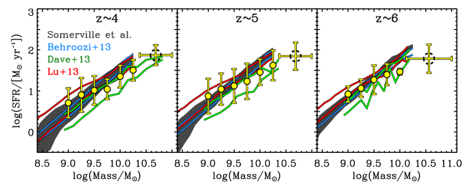
Figure 12 shows the scatter in the SFR–stellar mass relation for each of the models as compared to the observed median and scatter in the SFR at fixed stellar mass (with data and errors bars identical to those in Figure 11). For each model, the median and scatter in the SFR at fixed mass was computed in the same way as the data (with all models converted to a Salpeter (1955) IMF, as assumed in this work).

The SFR–mass relations from each model are in general agreement with each other and imply a tight relation between SFR and stellar mass exists for galaxies at high redshift. The SFR–mass relations from the models are also very similar to the observed relation derived from the data. Though some models predict a steeper slope of near unity ($a$$\simeq 1$), higher than measured in this work ($a$$\simeq 0.6$), the difference is negligible as it is within the errors. The observed offset in the zero point between the models and observations is likewise insignificant as the zero point is strongly anticorrelated with the slope in the linear fits of this work. In addition, from Figure 9 it was shown that the recovered SFRs from tests with the mock data tended to under- (over-) estimate the SFR of model galaxies with high (low) SFRs. No attempt was made to correct this for systematic. Therefore the similar offsets seen in Figure 12 between the high-SFR objects may imply that the data and SAMs are in even closer agreement.

As listed in Table 4, the scatter in the SFR at fixed mass is typically $0.1-0.2$ dex in the models, whereas the limits on the intrinsic scatter from the data are $\sigma(\log\mathrm{SFR})<0.2-0.3$ dex (see S 5.2.1). Therefore, both the observations and models support the conclusion that the SFR in galaxies at $3.5<z<6.5$ at fixed mass (for $\log M_{\star}/\mathrm{M}_{\odot}>9$ dex) scales nearly linearly with increasing stellar mass and does not vary by more than a factor of order 2. We explore the implication this has for the net gas accretion rate below in § 6.1.

6. Discussion

6.1. Implications of the SFR–Stellar Mass Relation

The fact that there is a tight SFR–stellar mass relation implies that the SFR scales almost linearly with stellar mass for the galaxies in our sample at $3.5<z<6.5$. Because the SFR is (to a coarse approximation) the time derivative of the stellar mass, this implies that the SFR is an increasing function with time. We explore this further below in § 6.2. Furthermore, the tightness of the scatter indicates that there is little variation in the SFR at fixed stellar mass. One caveat is that the SFRs are based on the galaxies’ UV luminosity. Therefore, the SFRs that we measure are the “time-averaged” over the time it takes for the UV luminosity in galaxies to respond to changes in their instantaneous SFR. For the UV luminosity this timescale is approximately 30-100 Myr (e.g., Salim et al., 2009). Recent simulations have shown that the scatter is highly sensitive to the timescale of the SFR indicator (Hopkins et al., 2014; Domínguez et al., 2014). Therefore, the tightness in the SFR–mass relation of this work is conditional on the timescale associated with UV SFRs. With that in mind, the scatter observed in this work implies that galaxies at fixed mass in our sample have similar star formation histories when averaged over this timescale.

The scatter in the SFR–mass relation has important implications for net interplay between gas accretion into halos and galaxy feedback and outflows at these redshifts. The gas-accretion rate is a crucial piece of physics in galaxy formation models, and measures of the scatter in the SFR–mass relation are therefore an important test to constrain simulations and SAMs. As discussed above, the SFR is expected to track the net accretion rate/outflow rate of baryonic gas into the galaxies’ dark-matter halos (Kereš et al., 2005; Dekel et al., 2009; Bouché et al., 2010; Lu et al., 2014). Because the SFR–mass relation is tight, it then follows that the gas accretion rate has little variation ($\sigma\sim 0.2-0.3$ dex, or a factor of $<$ 2) at fixed stellar mass. Therefore, this favors a relatively smooth gas accretion process for galaxies at $3.5<z<6.5$, at least above $\log M_{\star}/\mathrm{M}_{\odot}>9$ dex.

6.2. Evolution of the SFR

Figure 13.— Cumulative stellar mass functions in bins of redshift. No corrections have been applied for completeness, but Duncan et al. (2014) show these corrections are negligible for $\log M_{\star}/\mathrm{M}_{\odot}>9$ dex. The arrows and circles indicate the stellar mass evolution of the progenitors of galaxies with an evolving number density with $\log n(>M_{\star})$/Mpc${}^{-3}=-4$ at $z=3.5$ using the evolution parameterized by Behroozi et al. (2013a). We measure the SFR evolution of these galaxies. As we discuss below, we would have inferred a very similar evolution in SFR for galaxies selected at constant number density, with $\log n(>M_{\star})/$Mpc${}^{-3}=-3.7$, at all redshifts.

Figure 14.— The selection of galaxies according to the Behroozi et al. (2013a) evolving number density of $\log n(>M_{\star}$)/Mpc${}^{-3}=-4$ at $z=3.5$. The large salmon-colored circles show the median stellar mass evolution, and the dashed lines illustrate our sample selection of $\pm 0.25$ dex in stellar mass about these median values. We select all galaxies within these lines, and use them to derive the star formation history.

Figure 15.— The SFR history (the SFR as a function of redshift) for galaxies selected by their (evolving) number density to track the evolution in the progenitors of galaxies at $z=3.5$ with $\log n/\mathrm{Mpc}^{-3}=-4$. The galaxies from each redshift subsample $z=$ 4, 5, and 6 are indicated as blue, green, and orange points respectively. The larger salmon-colored circles and error bars show the median SFR and $\sigma_{\mathrm{MAD}}$ in bins of $\Delta z=0.5$. An average rising star formation history is derived for this redshift range that can be represented by a power law $\Psi=t^{\gamma}$ where $\gamma=1.4\pm 0.1$. This evolution is somewhat shallower than that found by Papovich et al. (2011), but consistent within the error budget.

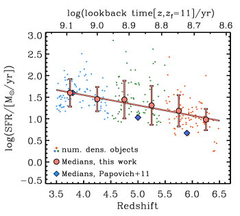
As discussed above, a tight, linear relation between SFR and stellar mass implies an SFR that increases with time. In this section, we study the SFR history directly to see if it is consistent with the observed SFR–stellar mass relation. This is achieved by tracking the evolution of the progenitors of $z=4$ galaxies by selecting galaxies at different redshifts based on their number density.

Many studies have shown that a constant (comoving) number-density selection can trace the progenitor and descendant evolution both to relatively low and high redshifts (e.g., van Dokkum et al., 2010; Papovich et al., 2011; Lundgren et al., 2014; Leja et al., 2013b; Patel et al., 2013; Tal et al., 2014). In addition, recent studies have suggested using an evolving number-density selection to better track the progenitor populations of galaxies (e.g., Leja et al., 2013a; Behroozi et al., 2013a). Here, we use the parameterization of Behroozi et al. (2013a), who provide simple functions to track the number density evolution of the progenitors of galaxies.

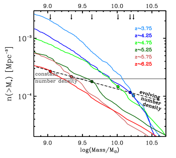
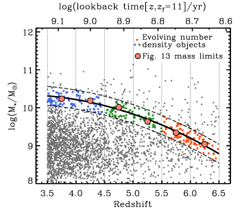
This number density evolution is used to select the progenitors of galaxies in our sample. Figure 13 shows the cumulative stellar mass functions for the galaxies in our $3.5<z<6.5$ CANDLES samples in bins of redshift. The results of Duncan et al. (2014) show that the objects in this field are complete for masses greater than $\log M_{\star}/\mathrm{M}_{\odot}=$ 8.55, 8.85, and 8.85 dex at $z\sim$ 4, 5 and 6 respectively. We assume a survey area of 170 arcmin² as described by Koekemoer et al. (2011) and the co-moving volume is calculated at each redshift assuming an uniform depth across each field. These cumulative functions are used to determine the stellar mass at which the galaxies of that redshift range achieve a given evolving number density as described by Behroozi et al. (2013a). As indicated in the figure, we take the galaxies with stellar mass $\log M_{\star}/\mathrm{M}_{\odot}=10.2$ dex at $z=3.75$, which have a number density of $\log n/\mathrm{Mpc}^{-3}=-4$, and identify the galaxies at higher redshift that have a stellar mass that corresponds to the appropriate (de-evolved) number density at that redshift.

Figure 14 illustrates our criteria to select objects according to an evolving number density. We use the Figure 13 stellar mass limits to find a best-fit curve across 3.5 $<z<$ 6.5. Then, we select objects from our data that are $\pm$ 0.25 dex in stellar mass about this relation. For the remainder of this work, we refer to these objects as “evolving number density–selected”. We will later compare these briefly to objects selected at “constant number density” as such samples have received attention in the recent literature.

Figure 15 shows the average SFR as a function of redshift for the evolving number density–selected galaxies. The SFR clearly increases as a function of time (decreasing redshift). We fit this evolution with a power law, $\Psi(t)\sim(t/\tau)^{\gamma}$ where $\gamma$ = 1.4 $\pm$ 0.1 and $\tau=92\pm 14$ Myr. If our sample is incomplete at low stellar masses ($\log M_{\star}/\mathrm{M}_{\odot}<9.5$ dex), then this would influence the measured power, $\gamma$. Based on Figure 13, the lower-mass objects will suffer greater incompleteness for objects of low SFR. This could mean that the intrinsic power-law slope is steeper than the one we measure here. We also note that we observe little difference between this evolution and that derived from using a constant-number density-selection.

Figure 16.— The median values of SFR and stellar mass relation from Figure 11 are shown, color coded by redshift. The gray region line is not a fit to the points, but is instead the implied relation (with errors) using the measured SFR history (from Fig. 15) derived by integrating that SFR history with the Bruzual & Charlot SPS models. For the $z=4$ galaxies with $\log M_{\star}/\mathrm{M}_{\odot}=10.2$ dex there is good agreement between the observed SFR–mass relation and the implied value from the SFR history. This is reassuring as the derived star formation history corresponds to the progenitors of galaxies of this mass at this redshift. At lower stellar masses, the SFR–mass relation implied from the derived star formation history underproduces the SFR, but we attribute this to the fact that the SFR history of lower-mass galaxies evolves less steeply with time.

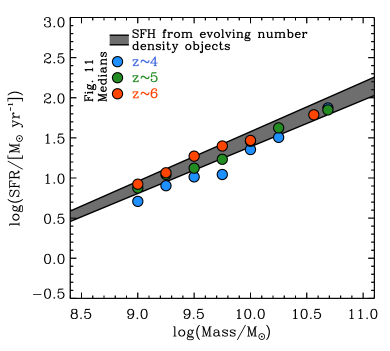
Lastly, we can explore whether the SFR evolution derived above produces an average SFR–mass relation as measured from the data. We took the SFR history derived above and compute the resulting stellar mass and SFR for a stellar population starting at $z=6$ and evolving to $z=4$ using the BC03 SPS models (see discussion in § 5.1 and bottom right panel of Figure 10). We plot the resulting SFR–mass relation in Figure 16 along with the medians derived above in Figure 11. Formally, the star formation history derived here corresponds to a galaxy with stellar mass $\log M_{\star}/\mathrm{M}_{\odot}=10.2$ dex at $z=3.75$. Looking only at that point, the SFR–mass relation inferred from the SFR history matches the SFR–mass relation at $z\sim 4$ remarkably well. (This is not circular because the stellar mass evolution is measured from the SFR evolution and not from the data itself.)

6.3. Evolution of the sSFR

Figure 17.— The evolution of the sSFR as a function of redshift for galaxies selected with constant stellar mass ($\pm$0.5 dex of $\log{}M_{\star}/\mathrm{M}_{\odot}=9$ dex). Grey points represent individual objects, while salmon-colored circles are medians in $\Delta z=0.5$ bins of redshift. The cyan curve shows a fit to the literature medians across all redshift. We find that at constant stellar mass, the sSFR gradually decreases over our redshift range. The other lines and shaded region correspond to model predictions as listed in the legend. The zero point and rate of evolution between the models and data are similar.

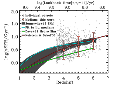
Lastly, we use our derived SFRs and stellar masses to study the evolution of the sSFR. We first explore the evolution with redshift at fixed stellar mass as this has received attention in the literature (even though it is clear that galaxies with such high SFRs will not remain at the same stellar mass over this redshift range). We then consider the evolution in sSFR for the evolving number density-selected sample described above, as this will better track the evolution in galaxy progenitors across this redshift range.

Figure 17 shows the evolution of the sSFR for objects selected with constant stellar mass: within $\pm$0.5 dex of $\log M_{\star}/\mathrm{M}_{\odot}$ = 9. The sSFR for objects at this stellar mass increases with increasing redshift, with high scatter. This evolution is consistent with hydrodynamic simulations (Davé et al., 2011b), SAMs (Somerville et al., Lu et al.), and other recent observational results from the literature (Stark et al., 2013; González et al., 2014).

Figure 18.— The evolution of the sSFR as a function of redshift for galaxies selected by their evolving number density to track the progenitors of galaxies at $z=3.5$ with $\log n/\mathrm{Mpc}^{-3}=-4$. The larger salmon-colored circles and error bars show the medians of $\log$ sSFR in bins of redshift. The other lines and shaded region correspond to model predictions as listed in the legend¹⁹.

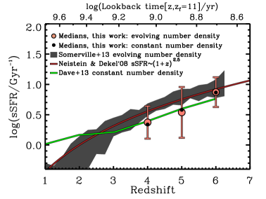
Figure 18 shows that the sSFR increases with redshift when galaxies are selected with an evolving number density. The evolution of the simple cosmological accretion models where sSFR$\sim\ (1+z)^{\phi=2.5}$ (e.g., Neistein & Dekel, 2008) is consistent with the sSFR evolution found in this work (Fig. 18), which has $\phi=3.4\pm 2.5$ from $z$=3.5 to $z$=6.5. There is a weak difference between the evolution of the evolving number density-selected sample and the sample at constant mass in Figure 17; the sSFR evolution for the evolving number density–selection is shifted to lower values as a function of redshift. This is basically a confirmation of the fact that the SFR–mass relation produces an sSFR that is nearly independent with stellar mass: sSFR = SFR / $M$ $\sim$ $M^{a-1}$, where sSFR $\sim M^{-(\approx 0.4)}$ using our results in Table 4. This implies that samples selected at constant stellar mass or an evolving stellar mass (from a number density selection) return only slightly different sSFR values because the sSFR is a slowly changing function with stellar mass, as recently found by Kelson (2014). Consequently, this permits mass-independent modeling of the specific accretion rate, and therefore the sSFR (see Dekel & Mandelker, 2014, for a detailed discussion).

One way to explain the slight offset of the observed sSFR to lower values than the predictions from the SAMs is that some feedback mechanism may be present to hinder SFR from tracing halo or stellar mass growth. Gabor & Bournaud (2014) recently showed that cold streams of gas can increase the velocity dispersion in star-forming disks. They show that at $z>$ 3 this increased turbulence causes the gas-mass to stay higher, but reduces the SFR / gas-mass by a factor of two. Assuming gas-mass traces the baryonic-mass in galaxies at $z>$ 3, then this could explain why the observed median sSFRs of this work are lower by about a factor of order two compared to other models.

7. Conclusions

In this work we use a photometric-redshift sample selected from the CANDELS GOODS-S field to study the average population of galaxies across the redshift range $3.5<z<6.5$. We present a Bayesian SED fitting procedure that takes advantage of the full posterior to determine the physical properties (stellar mass, SFR) of each galaxy. Our method incorporates effects of nebular emission lines and different dust attenuations, although we show that the effects of these different models are largely mitigated when the parameters are derived from posterior probability densities. This method is shown to have several advantageous over using best-fit parameter values from SED fits, including the fact that our method recovers stellar masses and SFRs from a SAM mock catalog.

We use the stellar masses and SFRs derived from the CANDELS photometry to study the evolution in the SFR–mass relation, SFR evolution, and sSFR evolution for galaxies at $3.5<z<6.5$. Our conclusions are the following:

• The ability to recover the slope, normalization, and scatter of the SFR–stellar mass relation is tested by taking advantage of mock catalogs and synthetic photometry of SAM galaxies. With a control sample of simulated data, we show that our Bayesian SED fitting procedure can well recover the SFR–stellar relation from complex star formation histories, although these tests are limited to the stochasticity of the histories in the simulations. Moreover, our procedure is less sensitive to stellar population template assumptions (such as the inclusion of nebular emission and the type of assumed attenuation prescription) than traditional methods.

• We find that from $3.5<z<6.5$ the star-forming galaxies in CANDELS follow a nearly unevolving correlation between SFR and stellar mass, parameterized as SFR $\sim$ M^a with $a$ = $0.54\pm 0.16$ at $z\sim 6$ and $0.70\pm 0.21$ at $z\sim 4$. The observed scatter in the SFR–stellar mass relation is small for galaxies with $\log M_{\star}/\hbox{M${}_{\odot}$}>9$ dex at all redshifts, at least on timescales associated with UV SFRs. This evolution requires a star formation history that increases with decreasing redshift (on average, the SFRs of individual galaxies rise with time). We note that our redshift range limits the data to cover rest-frame UV-to-optical wavelengths, and we defer the search for an underlying dust obscured population for future work.

• Comparing the observed $\log$ SFR scatter at fixed stellar mass with the scatter due to measurement uncertainties, the true intrinsic scatter is as much as $\sigma(\log$ SFR$)=$ 0.2$-$0.3 dex at all masses and redshifts. Assuming that the SFR is tied to the net gas inflow rate (including gas accretion and feedback), then the scatter in the gas inflow rate for star-forming galaxies over our stellar mass and redshift range is equally smooth, $\sigma$($\log$ Ṁ${}_{\text{gas}})<0.2-0.3$ dex, at least when averaged over the timescale of UV SFRs ($\sim$ 100 Myr).

• We measure the evolution in the SFR for galaxies from $z=6.5$ to 3.5 using an evolving number density selection to measure the evolution in galaxy progenitors that accounts for mergers between halos and variations in halo growth factors. For galaxies with $\log M_{\star}/\mathrm{M}_{\odot}=10.2$ dex at $z=4$, the star formation history follows $\Psi$/M_⊙  yr^-1 = $(t/\tau)^{\gamma}$ with $\gamma=1.4\pm 0.1$ and $\tau=92\pm 14$ Myr from $z=6.5$ to $z=3.5$. We further show that this star formation history reproduces the measured SFR–mass relation for galaxies at this mass and redshift.

• We show that the sSFR gradually increases with increasing redshift from $z=4$ to $z=6$, with only small qualitative differences if galaxies are selected at fixed stellar mass or by using an evolving number density. Broadly, the evolution in the sSFR is consistent with the theory of cosmological gas accretion where the SFR follows the net gas accretion rate.

Appendix A A. Changing the Assumed Star Formation History

Figure 19.— Results of SED fitting to synthetic photometry of recent SAM mock catalogs (Somerville et al)., now fitting to templates with exponentially rising star formation histories (similar to Fig. 9). The top panels show the log difference of measured-to-true SFRs. The derived SFRs are systematically higher than the true values, with high scatter. The middle panels show the ratio of the measured-to-true stellar masses. The stellar masses are systematically lower. The bottom panels show that the derived SFRs and stellar masses do not well recover the SFR–mass relation in the models when using exponentially rising star formation histories.

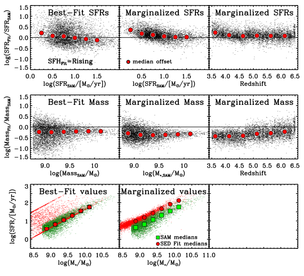
The SFRs and stellar masses used in this work are derived using SPS models with constant SFRs. In contrast, one of the main results of this work is that the high-redshift galaxies experience SFRs that increase monotonically with time, $\Psi\propto t^{1.4\pm 0.1}$. Naively, it would seem these statements are in conflict. Here we discuss how the star formation history affects the model interpretation, and we offer justification for the use of models with constant SFRs.

First, we tested SED fits with our Bayesian formalism that marginalize over a range of star formation histories, including those that rise with time, with $e$-folding times, $\tau=50$, 100, 300 Myr, and 100 Gyr (the long $e$-folding time approximates a constant SFR and keeps all the models handled identically in normalization by the BC03 software), where the star formation history is then defined as $\Psi\sim\exp^{t/\tau}$. We then use our Bayesian formalism to derive model parameters using the synthetic photometry from the galaxy mock catalog using the Somerville et al. SAM.

Figure 19 shows the SFRs and stellar masses measured from the synthetic photometry compared to the true model values using this large range of model parameters. This figure can be compared directly to Figure 9 above, which used models assuming only a constant star formation history. In comparison, the model parameters derived using the suite of histories that include rising SFRs produce stellar masses that are skewed low and SFRs that are skewed high compare to the true values. This appears to be unphysical.

Figure 20.— Top: The ratio of the best-fit stellar masses from model fits that include the effects of nebular emission lines (e.g., $f_{\mathrm{esc}}=0$) and exclude emission lines (e.g., $f_{\mathrm{esc}}=1$) for the objects in our CANDELS sample. Black points show the ratio of the best-fit values as a function of redshift, and the large red points show the medians in bins of redshift. Bottom: Ratio of best-fit SFRs from model fits with and without nebular emission lines. For galaxies with redshifts that place strong emission lines in one or more of the bandpasses (see Fig. 3), the best-fit SFRs and stellar masses can be reduced by up to 0.5 dex (factor of 3), with a median of 0.3 dex (factor of 2). In contrast, our Bayesian formalism finds that including nebular emission has only a small effect on the derived stellar masses and SFRs (Fig. 8).

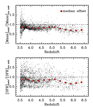
In hindsight, the reason for this is the following. In the BC03 models, the star formation history parameterization uses $e$-folding timescales (motivated by the exponentially decreasing models pioneered by Tinsley (1980)) and therefore the SFRs rise exponentially in time. Therefore, older stellar populations have unphysically increasing SFRs. At these late times, the models increase much faster than supported by observations (e.g., Papovich et al., 2001) or seen in simulations (e.g., Finlator et al., 2006). As a result, models with exponentially increasing SFRs must underproduce the stellar mass and overproduce the SFR to match the observed SED of galaxies. In contrast, the star formation histories of galaxies in our redshift range and in simulations can be approximately accurately as constant when averaged over the past $\sim$ 100 Myr, which includes the recently formed stars that dominate the luminosity-weighted age (see, e.g., Finlator et al., 2006). As a result, we do not consider the assumption of a constant star formation history to be a significant factor on the conclusions of this work. We note parenthetically that this is only true for the galaxies observed in this work because they are all heavily star-forming with high sSFRs; quiescent galaxies would require declining star formation histories.

Furthermore, our tests (discussed above in § 4.4 and Figure 9) show that SED fits using models with constant star formation reproduce accurately the SFRs and stellar masses from the models. Therefore, this work fixes the star formation history in fitting templates to be constant during the analysis of the CANDELS data. As the conclusions show, the galaxy populations require a star formation history with a rising SFR, but this evolution is slow and monotonic, $\Psi\propto t^{\gamma}$ (where $\gamma=1.4\pm 0.1$ from § 6.2 and Figure 15), which is not currently supported in a simple parameterization in the BC03 models. Nevertheless, in a future work, we will explore possible improvements in parameters using models with star formation histories that increase as a power law in time, as well as other more complex star formation histories.

Appendix B B. Stellar population synthesis fitting: Comparing Best-Fit Results

We compare between using the best-fit results from SED fitting procedures to using our Bayesian formalism to derive parameters from their posterior probability densities. In each subsection, we observe the offsets under different fitting template assumptions, including the effect of nebular emission lines and dust-attenuation prescription.

B.1. B.1 Effect of including nebular emission

The effects of including effects of nebular emission to the stellar templates are largely mitigated when using our Bayesian formalism (see Figure 8). In contrast, the nebular emission lines can strongly affect stellar masses and SFRs derived from best-fit model parameters. Figure 20 shows that in the redshift range of our galaxy sample, the presence (or absence) of an emission line in the ISAAC $K_{s}$, [3.6], and [4.5] bandpasses results in best-fit models that typically have lower SFRs and stellar masses by up to 0.5 dex (factor of 3). This is because a galaxy with a redder rest-frame UV-optical color requires either an older stellar population or heavier dust attenuation, with higher $M_{\star}/L$ ratios. Models where emission lines are present in the redder passbands reproduce the redder rest-frame UV-optical colors with lower stellar masses and SFRs. The effects of nebular emission are strongest in the redshift range that strong emission lines are present (see Fig. 3). The median decrease is up 0.3 dex (factor of 2) in both SFR and stellar mass for $5.5<z<6.5$. As discussed in the literature, this can affect the interpretation of the galaxies (Schaerer & de Barros, 2009, 2010; Schaerer et al., 2013; Ono et al., 2010; Finkelstein et al., 2011; Curtis-Lake et al., 2013; de Barros et al., 2014; Reddy et al., 2012; Stark et al., 2013; Tilvi et al., 2013).

It is worth noting that strength of the nebular emission lines is highly uncertain for several reasons. One clear reason is that the model must use some escape fraction of ionizing photons, which is allowed to range between $0\leq f_{\text{esc}}\leq 1$. Another uncertainty is that in our parameterization, the strength of line emission is tied to the age of the model stellar population, and age is less constrained in SED fitting (see, e.g., Papovich et al. (2001) and Fig. 5 above). Fits to galaxies using models with a starburst-like attenuation prescription (Calzetti et al., 2000) produce age distributions skewed heavily to the low ages (in some cases unphysically low as the ages are much less than a dynamical time, (e.g., Yan et al., 2006; Eyles et al., 2007; Schaerer & de Barros, 2009; de Barros et al., 2014; Reddy et al., 2012)). Both the escape fraction and inferred ages are poorly known quantities which cause the effect of nebular emission lines to likewise be poorly constrained, (see also, Verma et al., 2007; Oesch et al., 2013). For these reasons it is advantageous to use SED fitting that is not strongly influenced by the presence or absence of such lines. As we show above (§ 4.3 and Fig. 8), our Bayesian formalism is less affected by nebular emission lines in the models. Therefore, for the analysis in this paper we adopt models with $f_{\text{esc}}=0$. In a future work, we will consider fully marginalizing over a range of escape fraction, although it seems unlikely to change the conclusions here.

Figure 21.— Left:The ratio of stellar masses from best-fit models that assume SMC-like attenuation to those that assume a starburst-like attenuation as a function of best-fit mass. Small points show individual galaxies, where the color denotes the attenuation from the best-fit model assuming starburst-like dust. The large points show medians in bins of $d\log M_{\star}/\mathrm{M}_{\odot}$ = 0.5 dex. (We have excluded showing objects with best-fit models that have zero reddening, $A_{\mathrm{UV}}$=0, as these lie on the unity line.) At lower masses, the extinction prescription has little effect on the best-fit masses. At higher masses, $\log M_{\star}/\mathrm{M}_{\odot}>$ 10 dex, there is weak trend in that the best-fit models with SMC-like dust have lower stellar masses ($\sim$0.1 dex at $\log M_{\star}/\mathrm{M}_{\odot}\ \gtrsim$ 10.8 dex). This is likely related to the fact that higher-mass galaxies appear to have higher reddening (so presumably lower mass, dusty galaxies would also have the same trend in mass). Right: Ratio of the SFRs for the same best-fit models. Here there is a strong trend in SFRs from the best-fit models: as the SFR increases, there the models with starburst-like dust have significantly higher SFRs, by up to a 0.5 dex, with a median of $\sim$0.3 dex (factor of 2). Clearly the choice of dust attenuation prescription affects the interpretation of galaxy SFRs in the best-fit models. Nevertheless, as we show above in Figure 8, in our Bayesian formalism these differences are mitigated, and the dust attenuation prescription has negligible impact on the results here.

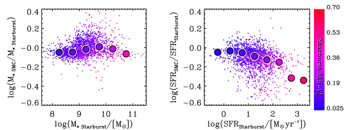
B.2. B.2 Dependence on attenuation prescription

Figure 21 shows the effects of the dust attenuation prescription on the stellar masses and SFRs from the best-fit models. The choice of dust attenuation prescription has a weak effect on stellar mass, where models using the SMC-like attenuation prescription have lower stellar masses by $\sim$0.1 dex in the median compared to the starburst-like dust attenuation (although the spread is larger, up to $\pm$0.2 dex).

The choice of dust attenuation prescription has a much stronger effect on the SFRs derived from best-fit models. Figure 21 shows that there is a strong trend in SFRs from the best-fit models: as the SFR increases, the models with starburst-like dust have significantly higher SFRs, by up to a 0.5 dex, with a median of $\sim$0.3 dex (factor of 2) compared to the best-fit solutions using an SMC-like dust. This is due to a combination of effects. First, there are high degeneracies between the inferred attenuation and age that arise from broadband SED fitting (discussed in the previous Appendix subsection). The assumed SFR depends on the stellar population age, especially at lower ages, where this leads to much higher ratios of in the SFR/$L_{1500}$ ratio (see Appendix of Reddy et al., 2012) compared to the value typically assumed in the Kennicutt (1998) relation which assumes ages greater than $10^{8}$ yr.

Dust extinction and age are degenerate (negatively covariant) in the SED modeling and models with starburst dust typically have lower best-fit ages (Papovich et al. 2001). Therefore, the effects of higher dust attenuation and higher SFR$/L_{1500}$ ratio both contribute to a larger SFR for the case of starburst-like dust. The differences between starburst-like and SMC-like dust models are highest for models with highest SFRs, as shown in Figure 21. For objects with the highest SFR, the difference between the two prescriptions can be as high as $\sim 0.7$ dex. Therefore, for best-fit models an assumed SMC-like attenuation causes starburst-attenuation-derived young, dusty, and high-SFR objects to be older, less dusty, and with lower SFR. This also reinforces the result of nebular emission in the Appendix above that simple template assumptions can significantly impact the best-fit SFR. Nevertheless, as we show above in Figure 8, in our Bayesian formalism these differences are mitigated, and the dust attenuation prescription has negligible impact on the results here.

For these reasons, this work assumed an SMC-like attenuation for all objects in our sample. If we otherwise had very reliable age estimates we might assume, as by Reddy et al. (2012), an “age”-dependent attenuation prescription, such that younger galaxies have SMC and older have starburst attenuation. However, the effects of nebular emission and assumed attenuation are strongest when adopting best-fit values. In contrast, we mitigate these effects by using the results from our Bayesian analysis, where the effects of changing dust attenuation prescription are minimized (see § 4).

B.3. B.3 Difference of Marginalized SFR compared to traditional methods

Figure 22.— A comparison between different methods to compute the SFR. The abscissa shows our adopted method, which uses the SFR from the attenuated luminosity of the photometric measurement closest to rest-frame 1500 Å, corrected for dust attenuation using the median $A_{\mathrm{UV}}$ from the marginalized posterior PDF (see Equation 5). The ordinate of the top panel compares our SFR to the SFR derived from the UV luminosity at L₁₅₀₀ and the UV slope, $\beta$, to correct for dust attenuation. The ordinate of the bottom panel compares our SFR toe the SFR from the best-fit stellar population model. In both cases the alternative SFRs show a large scatter, which can lead to significant biases. We favor using our method because our method reproduces the SFRs from the SAMs (see § 4.4 and Fig. 9), reducing some of this bias.

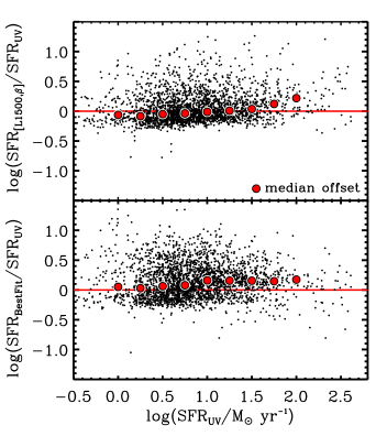
The method used in the work to derive UV SFRs for high redshift galaxies is different from the typical methods found in the literature. The common methods include using a dust correction based on the UV spectral slope, $f_{\lambda}\sim\lambda^{\beta}$, (Meurer et al., 1999; Madau et al., 1998; Kennicutt, 1998) and using the instantaneous SFR from the best-fit stellar population model. As shown in Figure 22, both of these alternative methods show high scatter when compared to the marginalized SFR from the method of this work.

The large scatter in Figure 22 is due to the fact that the scale of SFR is predominantly dependent on the treatment of the dust correction to UV luminosity, which is an unconstrained quantity in traditional SED fitting methods at high redshift. The Bayesian approach has the advantage in producing realistic ages, thereby reducing degeneracies with dust corrections. The median age for the SAM mock catalogs is $\log(t_{\text{age}})$= 8.48 $\pm$ 0.22 dex which resembles the distribution of marginalized ages found in this work for observed galaxies, $\log(t_{\text{age}})$= 8.73 $\pm$0.14 dex. Conversely, the distribution of best-fit ages is typically very dissimilar from SAM and simulation predictions. This is because best-fits typically find lowest $\chi^{2}$ at the extreme end of parameter space (youngest ages, highest extinction). As a result, the median best-fit ages are lower with higher scatter $\log(t_{\text{age}})$= 8.06 $\pm$ 0.94 dex. This scatter results from the degeneracies between the young, dusty and old, dust-free solutions of a given SED, and photometric uncertainties (which affect the accuracy of measuring the UV spectral slope, $\beta$) thus producing a wide range of acceptable SFRs.

In summary, when marginalizing over other nuisance parameters, the posterior on age returns more physical ages on the order of $\sim$350–750 Myr, reducing degeneracies in the derived dust corrections and thereby reducing the uncertainty in SFR. In addition, the method used in this work reproduces SFRs from semi-analytic models (see § 4.4), and is relatively unaffected by model variations such as extinction prescription and/or nebular emission lines. This is additional evidence to favor the Bayesian approach to derive physical properties.

Figure 23.— Top: the shapes of priors as a function of $\log$(age) (left) and UV attenuation (right). Our “fiducial” prior is what we adopt for the results of this work, while the flat priors are tests to study how the choice of prior affects the results. The dotted lines show the posterior of a given parameter for a single, example object assuming our fiducial prior. Bottom histograms of the inferred stellar population ages for a sample of 600 control objects from the Somerville et al. SAM. The red distribution is the “true” distribution from the SAM, while the yellow (solid, fiducial) and blue (dashed, flat) lines show the recovered distribution after fitting to the SAM fluxes assuming different priors. The thin black line shows the recovered values assuming the maximum likelihood solution, or “best-fit”. This figure emphasizes that best-fit solutions do not well recover the distribution of input ages and attenuations, and that our fiducial prior is preferred over a flat prior to recover stellar ages.

Figure 24.— Top: the same as the top of Fig. 23, shown for reference. Four additional test priors labeled A–D are shown and referred to in the text. Middle The slope and $\sigma$ scatter of the SFR–stellar mass relation for a sample of 600 control objects from the Somerville et al. SAM. The red is the “true” scatter from the SAM, while the yellow (solid, fiducial) and blue (dashed, flat) is the scatter after fitting to the SAM fluxes assuming different priors on age (left) and attenuation (right). Bottom: the $\sigma$ scatter of SFR in each stellar mass bin. Squares and triangles represent the scatter assuming our fiducial prior or a flat prior, respectively, while the diamonds represent the scatter of the input objects. This figure shows the recovery of the SFR–stellar mass relation under different priors, and that our fiducial prior is preferred over flat priors to recover the input SFR–stellar mass relation.

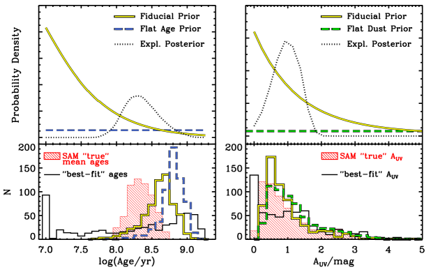
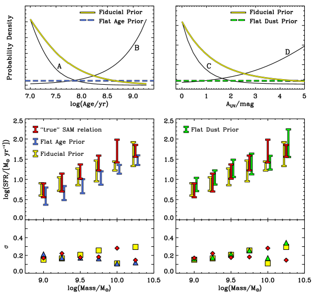
Appendix C C. Derivation of Prior

Here we describe the prior used in our SED fitting procedure and discuss tests to validate its use. The prior used in equation 3 was chosen to allow for an analytic derivation to the posterior probability densities that is straight-forward to calculate for each of the stellar population parameters, i.e., $p(t_{\text{age}}|D)$. Our prior-likelihood pair is therefore more easily computable (time efficient) and does not require more sophisticated methods such as a Markov Chain Monte Carlo. Our “fiducial” prior, which is used for the results of this work, is can be expressed as a sum over $i$ bands as,

$$p(\Theta^{\prime})\ =\ \left(\sum_{i=1}^{n}f_{\Theta}^{2}(\lambda_{i})/\sigma_{i}^{2}\right)^{1/2}$$ (C1)

where $\Theta^{\prime}$ represents the entire set of parameters, ${\Theta^{\prime}\ =(\Theta\{t_{\text{age}},\tau,A_{\text{UV}}\},\hbox{$\mathrm{M}_{\star}$})}$, and $f_{\Theta}$ is the model flux, unscaled by stellar mass. We express $\Theta$ as a separate parameter set from stellar mass because the prior in equation C1 is dependent on the fluxes of the gridded set of models, and independent of mass.

This prior is “flat” with respect to stellar mass, but spans the range of masses that the stellar population models can produce for a given set of data. Formally, the prior does depend on the other model parameters and the photometric uncertainties that are used to construct the stellar population synthesis models (age, dust, and star formation history). This is because the models are constructed using a discretized grid of stellar population parameters and a normalization that gives the mass. Since the prior is dependent on the fluxes of the gridded set of model parameters but not stellar mass, we distinguish $\Theta$ and $\mathrm{M}_{\star}$ separately in our equations. The shape of this fiducial prior is shown in the top panels of Figures 23 and 24.

In order to confirm that our posterior is constrained by the data and not dominated by the prior, we conducted several tests. First, we steadily increased the photometric uncertainties on the “mock” data from the SAM (lowered the S/N) and used that data as input to our procedure (a similar process as in S 4.4). This allows us to search for a characteristic S/N or stellar mass at which the SAM input values are poorly recovered, where here we adopt “poorly recovered” to mean systematically discrepant by a factor of 3 (0.5 dex) as compared to the input SAMs. We find that at S/N = 1 the recovered stellar masses of galaxies with log $\mathrm{M}_{\star}$/M_⊙= 9.75 are systematically higher by 0.5 dex. Such low S/N represents the scenario where the data have no power and the posterior reverts to the prior. Since all detected bands are typically of S/N $\gg$ 1, this test confirms that it is the likelihood computed from the data that is driving the shape of the posterior, and provides evidence that the conclusions of this work are not dominated by the prior.

In another test, we explored the effects of changing the assumed prior. We conducted this test on a control sample of 600 SAM objects that span the stellar masses and SFRs in the SAM for $z>$3.5. We then observed how well we could recover the age and attenuation distributions of the SAM when we changed the assumed prior to be flat in age or flat in dust. Figure 23 shows that using alternative priors shift the distributions of each parameter, but the prior does not overwhelm the likelihood from the data. For example, the flat age prior pushes the recovered age distribution away from the input age distribution because the flat age prior assigns more weight to older solutions than the fiducial prior. For both priors, the age distributions are old compared to the “true” values from the SAMs, but this is possibly a result of the differences between our assumed (slowly varying) star formation histories and the “physical” ones from the SAM. We consider the agreement between the “true” ages and recovered ages to be good.

The attenuation distributions are much less sensitive to the choice of prior. Figure 23 shows that there are only subtle differences between the distribution in $A_{\text{UV}}$ using our fiducial prior compared to those when using a flat prior. The figure also shows an example (“Expl.”) posterior for one object in the sample. This object shows that the probability density does not follow the prior. Moreover, this figure shows how either the fiducial or flat priors (for either parameter) do better at recovering the input distributions than the common method of taking the maximal likelihood, or “best-fit”, model.

Finally, we test how the above priors impact the recovery of the slope and scatter of the SFR–stellar mass relation for the control sample of SAM objects. Figure 24 shows the recovered $\sigma_{\text{MAD}}$ scatter about the median SFR in bins of stellar mass, calculated in the same manner as in Figure 11, but assuming different priors. The flat age prior shifts the distribution to older ages, and this effect propagates to SFR–stellar mass relation, shifting the SFR distribution to lower values. The flat age prior produces an SFR–stellar mass relation that is tightened and lower in normalization. One reason we disfavor the flat age prior is that the scatter in the SFR–stellar mass relation is even tighter than for our fiducial prior, and therefore the results from the fiducial prior are more conservative. Switching to a flat dust-prior has little effect on the slope and scatter in the SFR–stellar mass relation, given the scatter. We see similar effects on the results from the data when switching to these priors.

The top panels of Figure 24 also show a suite of alternative priors (labeled A-D) that were applied to the SAM control sample. A prior younger than our fiducial, such as prior A, assigns more weight to the likelihood of high SFRs at a given mass. This creates a scenario where galaxies are preferred to be young, maximal starbursts, causing the SFR–stellar mass relation to be artificially higher in normalization by $\sim$0.25 dex than the input SAM relation with an inflated scatter ($\langle\sigma\rangle>$ 0.05 dex) due to a wider range in mass-to-light ratios. Conversely, prior C and a “flat” age prior assign more weight to old age solutions than our fiducial prior. This results in a more narrow range of mass-to-light ratios, and therefore these priors produce a tighter SFR–stellar mass relation (${\langle\sigma\rangle\sim 0.16}$ dex) with lower normalization (lower SFR at a given mass than the input SAMs by $\sim$0.4 dex). On the other hand, our fiducial prior assigns more weight to younger age solutions, therefore avoiding an artificial decrease in SFR–stellar mass scatter, while not being too strong such that the recovered SFRs from the SAM are overestimated. We also find our procedure to be robust against changes to the attenuation prior, and find little change to the normalization slope and scatter when assuming the fiducial, flat, C, and D priors.

In summary, our tests indicate that the SFR-mass scatter is insensitive to the prior on dust and mildly sensitive to the prior on age. However, we conclude that our fiducial prior in age best recovers the age distribution and the SFR-stellar mass scatter of the SAM control sample and is straightforward to implement. Other priors that better reproduce the age distribution or the slope or scatter in SFR-stellar mass have SFRs at a given mass that are significantly off in normalization from the input SAMs.

Gabor14

References

- Anders & Fritze-v. Alvensleben (2003) Anders, P., & Fritze-v. Alvensleben, U. 2003, A&A, 401, 1063
- Ashby et al. (2013) Ashby, M. L. N., Willner, S. P., Fazio, G. G., et al. 2013, ApJ, 769, 80
- Atek et al. (2011) Atek, H., Siana, B., Scarlata, C., et al. 2011, ApJ, 743, 121
- Banerji et al. (2013) Banerji, M., Glazebrook, K., Blake, C., et al. 2013, MNRAS, 431, 2209
- Beers et al. (1990) Beers, T. C., Flynn, K., & Gebhardt, K. 1990, AJ, 100, 32
- Behroozi et al. (2013a) Behroozi, P. S., Marchesini, D., Wechsler, R. H., et al. 2013a, ApJ, 777, L10
- Behroozi et al. (2013b) Behroozi, P. S., Wechsler, R. H., & Conroy, C. 2013b, ApJ, 770, 57
- Behroozi et al. (2013c) Behroozi, P. S., Wechsler, R. H., & Wu, H.-Y. 2013c, ApJ, 762, 109
- Behroozi et al. (2013d) Behroozi, P. S., Wechsler, R. H., Wu, H.-Y., et al. 2013d, ApJ, 763, 18
- Birnboim & Dekel (2003) Birnboim, Y., & Dekel, A. 2003, MNRAS, 345, 349
- Bolton & Haehnelt (2007) Bolton, J. S., & Haehnelt, M. G. 2007, MNRAS, 382, 325
- Bouché et al. (2010) Bouché, N., Dekel, A., Genzel, R., et al. 2010, ApJ, 718, 1001
- Brammer et al. (2008) Brammer, G. B., van Dokkum, P. G., & Coppi, P. 2008, ApJ, 686, 1503
- Brammer et al. (2013) Brammer, G. B., van Dokkum, P. G., Illingworth, G. D., et al. 2013, ApJ, 765, L2
- Bridge et al. (2010) Bridge, C. R., Teplitz, H. I., Siana, B., et al. 2010, ApJ, 720, 465
- Bruzual & Charlot (2003) Bruzual, G., & Charlot, S. 2003, MNRAS, 344, 1000
- Buat et al. (2014) Buat, V., Heinis, S., Boquien, M., et al. 2014, A&A, 561, A39
- Calzetti et al. (2000) Calzetti, D., Armus, L., Bohlin, R. C., et al. 2000, ApJ, 533, 682
- Cattaneo et al. (2011) Cattaneo, A., Mamon, G. A., Warnick, K., & Knebe, A. 2011, A&A, 533, A5
- Ceverino et al. (2010) Ceverino, D., Dekel, A., & Bournaud, F. 2010, MNRAS, 404, 2151
- Chabrier (2003) Chabrier, G. 2003, PASP, 115, 763
- Charlot & Fall (2000) Charlot, S., & Fall, S. M. 2000, ApJ, 539, 718
- Chevallard et al. (2013) Chevallard, J., Charlot, S., Wandelt, B., & Wild, V. 2013, MNRAS, 432, 2061
- Conroy & Gunn (2010) Conroy, C., & Gunn, J. E. 2010, ApJ, 712, 833
- Conroy et al. (2009) Conroy, C., Gunn, J. E., & White, M. 2009, ApJ, 699, 486
- Curtis-Lake et al. (2013) Curtis-Lake, E., McLure, R. J., Dunlop, J. S., et al. 2013, MNRAS, 429, 302
- Daddi et al. (2007) Daddi, E., Dickinson, M., Morrison, G., et al. 2007, ApJ, 670, 156
- Dahlen et al. (2013) Dahlen, T., Mobasher, B., Faber, S. M., et al. 2013, ApJ, 775, 93
- Davé (2008) Davé, R. 2008, MNRAS, 385, 147
- Davé et al. (2011a) Davé, R., Finlator, K., & Oppenheimer, B. D. 2011a, MNRAS, 416, 1354
- Davé et al. (2013) Davé, R., Katz, N., Oppenheimer, B. D., Kollmeier, J. A., & Weinberg, D. H. 2013, MNRAS, 434, 2645
- Davé et al. (2011b) Davé, R., Oppenheimer, B. D., & Finlator, K. 2011b, MNRAS, 415, 11
- de Barros et al. (2014) de Barros, S., Schaerer, D., & Stark, D. P. 2014, A&A, 563, A81
- Dekel & Mandelker (2014) Dekel, A., & Mandelker, N. 2014, MNRAS, 444, 2071
- Dekel et al. (2009) Dekel, A., Birnboim, Y., Engel, G., et al. 2009, Nature, 457, 451
- Dickinson (1998) Dickinson, M. 1998, in The Hubble Deep Field, ed. M. Livio, S. M. Fall, & P. Madau (New York: Cambridge Univ. Press), 219
- Domínguez et al. (2014) Domínguez, A., Siana, B., Brooks, A. M., et al. 2014, ArXiv 1408.5788
- Donley et al. (2012) Donley, J. L., Koekemoer, A. M., Brusa, M., et al. 2012, ApJ, 748, 142
- Drory et al. (2004) Drory, N., Bender, R., & Hopp, U. 2004, ApJ, 616, L103
- Duncan et al. (2014) Duncan, K., Conselice, C. J., Mortlock, A., et al. 2014, MNRAS, 444, 2960
- Dunkley et al. (2009) Dunkley, J., Komatsu, E., Nolta, M. R., et al. 2009, ApJS, 180, 306
- Dunne et al. (2009) Dunne, L., Ivison, R. J., Maddox, S., et al. 2009, MNRAS, 394, 3
- Dutton et al. (2010) Dutton, A. A., van den Bosch, F. C., & Dekel, A. 2010, MNRAS, 405, 1690
- Erb et al. (2010) Erb, D. K., Pettini, M., Shapley, A. E., et al. 2010, ApJ, 719, 1168
- Erb et al. (2006a) Erb, D. K., Shapley, A. E., Pettini, M., et al. 2006a, ApJ, 644, 813
- Erb et al. (2006b) Erb, D. K., Steidel, C. C., Shapley, A. E., et al. 2006b, ApJ, 647, 128
- Eyles et al. (2007) Eyles, L. P., Bunker, A. J., Ellis, R. S., et al. 2007, MNRAS, 374, 910
- Faucher-Giguère et al. (2011) Faucher-Giguère, C.-A., Kereš, D., & Ma, C.-P. 2011, MNRAS, 417, 2982
- Ferland et al. (1998) Ferland, G. J., Korista, K. T., Verner, D. A., et al. 1998, PASP, 110, 761
- Finkelstein et al. (2011) Finkelstein, S. L., Hill, G. J., Gebhardt, K., et al. 2011, ApJ, 729, 140
- Finkelstein et al. (2012a) Finkelstein, S. L., Papovich, C., Ryan, R. E., et al. 2012a, ApJ, 758, 93
- Finkelstein et al. (2012b) Finkelstein, S. L., Papovich, C., Salmon, B., et al. 2012b, ApJ, 756, 164
- Finlator et al. (2007) Finlator, K., Davé, R., & Oppenheimer, B. D. 2007, MNRAS, 376, 1861
- Finlator et al. (2006) Finlator, K., Davé, R., Papovich, C., & Hernquist, L. 2006, ApJ, 639, 672
- Finlator et al. (2011) Finlator, K., Oppenheimer, B. D., & Davé, R. 2011, MNRAS, 410, 1703
- Fontana et al. (2004) Fontana, A., Pozzetti, L., Donnarumma, I., et al. 2004, A&A, 424, 23
- Forbes et al. (2014) Forbes, J. C., Krumholz, M. R., Burkert, A., & Dekel, A. 2014, MNRAS, 443, 168
- Förster Schreiber et al. (2004) Förster Schreiber, N. M., van Dokkum, P. G., Franx, M., et al. 2004, ApJ, 616, 40
- Gabor & Bournaud (2014) Gabor, J. M., & Bournaud, F. 2014, MNRAS, 437, L56
- Giavalisco (2002) Giavalisco, M. 2002, ARA&A, 40, 579
- González et al. (2014) González, V., Bouwens, R., Illingworth, G., et al. 2014, ApJ, 781, 34
- González et al. (2011) González, V., Labbé, I., Bouwens, R. J., et al. 2011, ApJ, 735, L34
- González et al. (2010) —. 2010, ApJ, 713, 115
- Grogin et al. (2011) Grogin, N. A., Kocevski, D. D., Faber, S. M., et al. 2011, ApJS, 197, 35
- Guo et al. (2013) Guo, Y., Ferguson, H. C., Giavalisco, M., et al. 2013, ApJS, 207, 24
- Guseva et al. (2006) Guseva, N. G., Izotov, Y. I., & Thuan, T. X. 2006, ApJ, 644, 890
- Hopkins et al. (2014) Hopkins, P. F., Kereš, D., Oñorbe, J., et al. 2014, MNRAS, 445, 581
- Ilbert et al. (2010) Ilbert, O., Salvato, M., Le Floc’h, E., et al. 2010, ApJ, 709, 644
- Inoue (2011) Inoue, A. K. 2011, MNRAS, 415, 2920
- Jarosik et al. (2011) Jarosik, N., Bennett, C. L., Dunkley, J., et al. 2011, ApJS, 192, 14
- Jones et al. (2013) Jones, T. A., Ellis, R. S., Schenker, M. A., & Stark, D. P. 2013, ApJ, 779, 52
- Katz et al. (2003) Katz, N., Keres, D., Dave, R., & Weinberg, D. H. 2003, in Astrophysics and Space Science Library, Vol. 281, The IGM/Galaxy Connection. The Distribution of Baryons at z=0, ed. J. L. Rosenberg & M. E. Putman (Dordrecht:Kluwer: Astrophysics and Space Science Library), 185
- Kauffmann et al. (2003) Kauffmann, G., Heckman, T. M., White, S. D. M., et al. 2003, MNRAS, 341, 33
- Kelson (2014) Kelson, D. D. 2014, ArXiv 1406.5191
- Kennicutt (1998) Kennicutt, Jr., R. C. 1998, ARA&A, 36, 189
- Kereš et al. (2005) Kereš, D., Katz, N., Weinberg, D. H., & Davé, R. 2005, MNRAS, 363, 2
- Klypin et al. (2011) Klypin, A. A., Trujillo-Gomez, S., & Primack, J. 2011, ApJ, 740, 102
- Koekemoer et al. (2011) Koekemoer, A. M., Faber, S. M., Ferguson, H. C., et al. 2011, ApJS, 197, 36
- Komatsu et al. (2009) Komatsu, E., Dunkley, J., Nolta, M. R., et al. 2009, ApJS, 180, 330
- Kriek & Conroy (2013) Kriek, M., & Conroy, C. 2013, ApJ, 775, L16
- Kriek et al. (2010) Kriek, M., Labbé, I., Conroy, C., et al. 2010, ApJ, 722, L64
- Labbé et al. (2006) Labbé, I., Bouwens, R., Illingworth, G. D., & Franx, M. 2006, ApJ, 649, L67
- Laidler et al. (2007) Laidler, V. G., Papovich, C., Grogin, N. A., et al. 2007, PASP, 119, 1325
- Lee et al. (2009) Lee, K.-S., Giavalisco, M., Conroy, C., et al. 2009, ApJ, 695, 368
- Lee et al. (2006) Lee, K.-S., Giavalisco, M., Gnedin, O. Y., et al. 2006, ApJ, 642, 63
- Lee et al. (2011) Lee, K.-S., Dey, A., Reddy, N., et al. 2011, ApJ, 733, 99
- Lee et al. (2012) Lee, K.-S., Ferguson, H. C., Wiklind, T., et al. 2012, ApJ, 752, 66
- Lee et al. (2010) Lee, S.-K., Ferguson, H. C., Somerville, R. S., Wiklind, T., & Giavalisco, M. 2010, ApJ, 725, 1644
- Leitherer & Heckman (1995) Leitherer, C., & Heckman, T. M. 1995, ApJS, 96, 9
- Leja et al. (2013a) Leja, J., van Dokkum, P., & Franx, M. 2013a, ApJ, 766, 33
- Leja et al. (2013b) Leja, J., van Dokkum, P. G., Momcheva, I., et al. 2013b, ApJ, 778, L24
- Lu et al. (2014) Lu, Y., Mo, H. J., Lu, Z., Katz, N., & Weinberg, M. D. 2014, MNRAS, 443, 1252
- Lu et al. (2013) Lu, Y., Wechsler, R. H., Somerville, R. S., et al. 2013, ArXiv 1312.3233
- Lundgren et al. (2014) Lundgren, B. F., van Dokkum, P., Franx, M., et al. 2014, ApJ, 780, 34
- Madau et al. (1998) Madau, P., Pozzetti, L., & Dickinson, M. 1998, ApJ, 498, 106
- Magdis et al. (2010) Magdis, G. E., Rigopoulou, D., Huang, J.-S., & Fazio, G. G. 2010, MNRAS, 401, 1521
- Maiolino et al. (2008) Maiolino, R., Nagao, T., Grazian, A., et al. 2008, A&A, 488, 463
- Malkan et al. (2003) Malkan, M., Webb, W., & Konopacky, Q. 2003, ApJ, 598, 878
- Man et al. (2014) Man, A. W. S., Greve, T. R., Toft, S., et al. 2014, ArXiv 1411.2870
- Mannucci et al. (2009) Mannucci, F., Cresci, G., Maiolino, R., et al. 2009, MNRAS, 398, 1915
- Maraston (2005) Maraston, C. 2005, MNRAS, 362, 799
- Maraston et al. (2010) Maraston, C., Pforr, J., Renzini, A., et al. 2010, MNRAS, 407, 830
- Marchesini et al. (2009) Marchesini, D., van Dokkum, P. G., Förster Schreiber, N. M., et al. 2009, ApJ, 701, 1765
- Meiksin (2006) Meiksin, A. 2006, MNRAS, 365, 807
- Melbourne et al. (2012) Melbourne, J., Williams, B. F., Dalcanton, J. J., et al. 2012, ApJ, 748, 47
- Meurer et al. (1999) Meurer, G. R., Heckman, T. M., & Calzetti, D. 1999, ApJ, 521, 64
- Michałowski et al. (2012) Michałowski, M. J., Dunlop, J. S., Cirasuolo, M., et al. 2012, A&A, 541, A85
- Mitchell et al. (2013) Mitchell, P. D., Lacey, C. G., Baugh, C. M., & Cole, S. 2013, MNRAS, 435, 87
- Mobasher et al. (in prep.) Mobasher, B., , & . in prep., ApJ
- Mollá et al. (2009) Mollá, M., García-Vargas, M. L., & Bressan, A. 2009, MNRAS, 398, 451
- Moustakas et al. (2013) Moustakas, J., Coil, A. L., Aird, J., et al. 2013, ApJ, 767, 50
- Murali et al. (2002) Murali, C., Katz, N., Hernquist, L., Weinberg, D. H., & Davé, R. 2002, ApJ, 571, 1
- Muzzin et al. (2013) Muzzin, A., Marchesini, D., Stefanon, M., et al. 2013, ApJ, 777, 18
- Neistein & Dekel (2008) Neistein, E., & Dekel, A. 2008, MNRAS, 383, 615
- Nestor et al. (2011) Nestor, D. B., Shapley, A. E., Steidel, C. C., & Siana, B. 2011, ApJ, 736, 18
- Noeske et al. (2007) Noeske, K. G., Weiner, B. J., Faber, S. M., et al. 2007, ApJ, 660, L43
- Oesch et al. (2013) Oesch, P. A., Labbé, I., Bouwens, R. J., et al. 2013, ApJ, 772, 136
- Oke & Gunn (1983) Oke, J. B., & Gunn, J. E. 1983, ApJ, 266, 713
- Oliver et al. (2010) Oliver, S., Frost, M., Farrah, D., et al. 2010, MNRAS, 405, 2279
- Ono et al. (2010) Ono, Y., Ouchi, M., Shimasaku, K., et al. 2010, ApJ, 724, 1524
- Oppenheimer & Davé (2008) Oppenheimer, B. D., & Davé, R. 2008, MNRAS, 387, 577
- Osterbrock & Ferland (2006) Osterbrock, D. E., & Ferland, G. J. 2006, Astrophysics of gaseous nebulae and active galactic nuclei (Sausalito, CA: University Science Books)
- Pacifici et al. (2012) Pacifici, C., Charlot, S., Blaizot, J., & Brinchmann, J. 2012, MNRAS, 421, 2002
- Padovani et al. (2011) Padovani, P., Miller, N., Kellermann, K. I., et al. 2011, ApJ, 740, 20
- Pannella et al. (2009) Pannella, M., Carilli, C. L., Daddi, E., et al. 2009, ApJ, 698, L116
- Papovich et al. (2001) Papovich, C., Dickinson, M., & Ferguson, H. C. 2001, ApJ, 559, 620
- Papovich et al. (2011) Papovich, C., Finkelstein, S. L., Ferguson, H. C., Lotz, J. M., & Giavalisco, M. 2011, MNRAS, 412, 1123
- Papovich et al. (2006) Papovich, C., Moustakas, L. A., Dickinson, M., et al. 2006, ApJ, 640, 92
- Patel et al. (2013) Patel, S. G., van Dokkum, P. G., Franx, M., et al. 2013, ApJ, 766, 15
- Pei (1992) Pei, Y. C. 1992, ApJ, 395, 130
- Raiter et al. (2010) Raiter, A., Schaerer, D., & Fosbury, R. A. E. 2010, A&A, 523, A64
- Reddy et al. (2012) Reddy, N. A., Pettini, M., Steidel, C. C., et al. 2012, ApJ, 754, 25
- Reddy et al. (2006) Reddy, N. A., Steidel, C. C., Fadda, D., et al. 2006, ApJ, 644, 792
- Reines et al. (2010) Reines, A. E., Nidever, D. L., Whelan, D. G., & Johnson, K. E. 2010, ApJ, 708, 26
- Renzini (2009) Renzini, A. 2009, MNRAS, 398, L58
- Rodighiero et al. (2010) Rodighiero, G., Cimatti, A., Gruppioni, C., et al. 2010, A&A, 518, L25
- Salim et al. (2009) Salim, S., Dickinson, M., Michael Rich, R., et al. 2009, ApJ, 700, 161
- Salpeter (1955) Salpeter, E. E. 1955, ApJ, 121, 161
- Sawicki (2012) Sawicki, M. 2012, MNRAS, 421, 2187
- Sawicki & Yee (1998) Sawicki, M., & Yee, H. K. C. 1998, AJ, 115, 1329
- Schaerer et al. (2014) Schaerer, D., Boone, F., Zamojski, M., et al. 2014, ArXiv 1407.5793
- Schaerer & de Barros (2009) Schaerer, D., & de Barros, S. 2009, A&A, 502, 423
- Schaerer & de Barros (2010) —. 2010, A&A, 515, A73
- Schaerer et al. (2013) Schaerer, D., de Barros, S., & Sklias, P. 2013, A&A, 549, A4
- Schreiber et al. (2014) Schreiber, C., Pannella, M., Elbaz, D., et al. 2014, ArXiv 1409.5433
- Shapley et al. (2001) Shapley, A. E., Steidel, C. C., Adelberger, K. L., et al. 2001, ApJ, 562, 95
- Shapley et al. (2005) Shapley, A. E., Steidel, C. C., Erb, D. K., et al. 2005, ApJ, 626, 698
- Shim et al. (2011) Shim, H., Chary, R.-R., Dickinson, M., et al. 2011, ApJ, 738, 69
- Siana et al. (2007) Siana, B., Teplitz, H. I., Colbert, J., et al. 2007, ApJ, 668, 62
- Siana et al. (2010) Siana, B., Teplitz, H. I., Ferguson, H. C., et al. 2010, ApJ, 723, 241
- Somerville et al. (2012) Somerville, R. S., Gilmore, R. C., Primack, J. R., & Domínguez, A. 2012, MNRAS, 423, 1992
- Somerville et al. (2008) Somerville, R. S., Hopkins, P. F., Cox, T. J., Robertson, B. E., & Hernquist, L. 2008, MNRAS, 391, 481
- Song et al. (2014) Song, M., Finkelstein, S. L., Gebhardt, K., et al. 2014, ApJ, 791, 3
- Speagle et al. (2014) Speagle, J. S., Steinhardt, C. L., Capak, P. L., & Silverman, J. D. 2014, ApJS, 214, 15
- Spitler et al. (2014) Spitler, L. R., Straatman, C. M. S., Labbé, I., et al. 2014, ApJ, 787, L36
- Springel & Hernquist (2003) Springel, V., & Hernquist, L. 2003, MNRAS, 339, 289
- Springel et al. (2005) Springel, V., White, S. D. M., Jenkins, A., et al. 2005, Nature, 435, 629
- Stark et al. (2009) Stark, D. P., Ellis, R. S., Bunker, A., et al. 2009, ApJ, 697, 1493
- Stark et al. (2013) Stark, D. P., Schenker, M. A., Ellis, R., et al. 2013, ApJ, 763, 129
- Steidel et al. (1999) Steidel, C. C., Adelberger, K. L., Giavalisco, M., Dickinson, M., & Pettini, M. 1999, ApJ, 519, 1
- Steinhardt et al. (2014) Steinhardt, C. L., Speagle, J. S., Capak, P., et al. 2014, ApJ, 791, L25
- Storey & Hummer (1995) Storey, P. J., & Hummer, D. G. 1995, MNRAS, 272, 41
- Straatman et al. (2014) Straatman, C. M. S., Labbé, I., Spitler, L. R., et al. 2014, ApJ, 783, L14
- Tal et al. (2014) Tal, T., Dekel, A., Oesch, P., et al. 2014, ApJ, 789, 164
- Tilvi et al. (2013) Tilvi, V., Papovich, C., Tran, K.-V. H., et al. 2013, ApJ, 768, 56
- Tinsley (1980) Tinsley, B. M. 1980, Fund. Cosmic Phys., 5, 287
- van der Wel et al. (2011) van der Wel, A., Straughn, A. N., Rix, H.-W., et al. 2011, ApJ, 742, 111
- van Dokkum et al. (2010) van Dokkum, P. G., Whitaker, K. E., Brammer, G., et al. 2010, ApJ, 709, 1018
- Verma et al. (2007) Verma, A., Lehnert, M. D., Förster Schreiber, N. M., Bremer, M. N., & Douglas, L. 2007, MNRAS, 377, 1024
- Walcher et al. (2011) Walcher, J., Groves, B., Budavári, T., & Dale, D. 2011, Ap&SS, 331, 1
- Wiersma et al. (2009) Wiersma, R. P. C., Schaye, J., & Smith, B. D. 2009, MNRAS, 393, 99
- Wuyts et al. (2009) Wuyts, S., Franx, M., Cox, T. J., et al. 2009, ApJ, 696, 348
- Wuyts et al. (2007) Wuyts, S., Labbé, I., Franx, M., et al. 2007, ApJ, 655, 51
- Wuyts et al. (2011) Wuyts, S., Förster Schreiber, N. M., Lutz, D., et al. 2011, ApJ, 738, 106
- Wyithe et al. (2014) Wyithe, J. S. B., Loeb, A., & Oesch, P. A. 2014, MNRAS, 439, 1326
- Xue et al. (2011) Xue, Y. Q., Luo, B., Brandt, W. N., et al. 2011, ApJS, 195, 10
- Yan et al. (2006) Yan, H., Dickinson, M., Giavalisco, M., et al. 2006, ApJ, 651, 24
- Zackrisson et al. (2008) Zackrisson, E., Bergvall, N., & Leitet, E. 2008, ApJ, 676, L9
- Zackrisson et al. (2001) Zackrisson, E., Bergvall, N., Olofsson, K., & Siebert, A. 2001, A&A, 375, 814
- Zibetti et al. (2013) Zibetti, S., Gallazzi, A., Charlot, S., Pierini, D., & Pasquali, A. 2013, MNRAS, 428, 1479