Suprathermal Electrons in the Solar Corona: Can Nonlocal Transport Explain Heliospheric Charge States?

Abstract

There have been several ideas proposed to explain how the Sun’s corona is heated and how the solar wind is accelerated. Some models assume that open magnetic field lines are heated by Alfvén waves driven by photospheric motions and dissipated after undergoing a turbulent cascade. Other models posit that much of the solar wind’s mass and energy is injected via magnetic reconnection from closed coronal loops. The latter idea is motivated by observations of reconnecting jets and also by similarities of ion composition between closed loops and the slow wind. Wave/turbulence models have also succeeded in reproducing observed trends in ion composition signatures versus wind speed. However, the absolute values of the charge-state ratios predicted by those models tended to be too low in comparison with observations. This letter refines these predictions by taking better account of weak Coulomb collisions for coronal electrons, whose thermodynamic properties determine the ion charge states in the low corona. A perturbative description of nonlocal electron transport is applied to an existing set of wave/turbulence models. The resulting electron velocity distributions in the low corona exhibit mild suprathermal tails characterized by “kappa” exponents between 10 and 25. These suprathermal electrons are found to be sufficiently energetic to enhance the charge states of oxygen ions, while maintaining the same relative trend with wind speed that was found when the distribution was assumed to be Maxwellian. The updated wave/turbulence models are in excellent agreement with solar wind ion composition measurements.

1. Introduction

The existence of the solar wind, a continuous outflow of charged particles from the Sun, is believed to be a direct result of the heating of plasma to temperatures of order $10^{6}$ K in the solar corona (Parker, 1958a). However, the physical processes responsible for the wind and the corona have not yet been identified conclusively (see, e.g., Marsch, 2006; Cranmer, 2009; Parnell & De Moortel, 2012). Much of the heliospheric plasma is of sufficiently low density to make particle–particle collisions infrequent. This means that some aspects of particle distributions measured in interplanetary space may carry information about the distant coronal heating. For example, the ionization states of most heavy ions are believed to be “frozen in” low in the corona and remain constant between heights of a few solar radii ($R_{\odot}$) and 1 AU. Above a certain point in the solar atmosphere, the ions collide with virtually no electrons and thus do not undergo any additional ionization or recombination (Hundhausen et al., 1968; Owocki et al., 1983)

Charge states measured at 1 AU have been used as indirect probes of the near-Sun plasma, with coronal electron temperatures $T_{e}\approx 1.5$ MK often being inferred (Geiss et al., 1995; Ko et al., 1997). However, spectroscopic measurements of temperature-sensitive emission line ratios typically gave $T_{e}\lesssim 0.9$ MK at the heights where freezing-in should take place. Esser & Edgar (2000, 2001) found that this discrepancy may disappear if either: (1) electrons have non-Maxwellian velocity distribution functions (VDFs), or (2) ions of different charge states flow with different speeds in the corona. More recent comparisons of spectroscopic and in situ measurements (e.g., Landi et al., 2012b; Ko et al., 2014) continue to attempt to reconcile these observations, but no single model has been found that explains everything.

Although there is no direct evidence for ion–ion differential streaming in the corona, there are hints that the electrons may have non-Maxwellian VDFs. Some earlier studies appeared to rule out the existence of suprathermal electrons at low coronal heights (Anderson et al., 1996; Ko et al., 1996), but the evidence may be starting to swing in the other direction (e.g., Ralchenko et al., 2007; Kulinová et al., 2011). Theoretically, a suprathermal electron “tail” may be the natural outcome of the dissipation of turbulent plasma fluctuations (Roberts & Miller, 1998; Viñas et al., 2000; Yoon et al., 2006) or the ballistic acceleration of coronal jets (Feng et al., 2012). Scudder (1992) suggested that any small nonthermal tail in the lower atmosphere can be amplified in the corona by gravitational filtration (see also Parker, 1958b; Levine, 1974).

Another possibly important source of non-Maxwellian VDFs may be the nonlocal transport of electrons through regions of weak collisionality. Because of the complex velocity dependence of Coulomb collisions, the electron distribution at one heliocentric distance depends on the properties of electrons over a range of surrounding distances. Ogilvie & Scudder (1978) suggested that suprathermal “halo” electrons seen at 1 AU are likely to be the remnant of a hot coronal VDF. Scudder & Olbert (1979) provided a straightforward model—reminiscent of radiative transfer in astrophysics—for estimating the magnitude of these effects in the coupled corona–heliosphere system.

This letter explores the consequences of nonlocal electron transport on the formation of the frozen-in charge states (e.g., O⁺⁷ and O⁺⁶) in an existing model of turbulent coronal heating and solar wind acceleration. Cranmer et al. (2007) found that the assumption of Maxwellian electrons resulted in values of the O⁺⁷/O⁺⁶ ionization state ratio that were too low by about an order of magnitude in comparison to observations. Section 2 applies the Scudder & Olbert (1979) transport framework to a representative fast-wind model. Section 3 shows how mild suprathermal enhancements at $r\approx 1.02\,R_{\odot}$, that result from collisional transport, appear to be sufficient to increase the frozen-in ionization states to the observed levels. Section 4 summarizes the results and gives suggestions for future improvements.

2. Nonlocal Model of Electron Transport

Cranmer et al. (2007) presented steady-state solutions to the conservation equations of mass, momentum, and energy for superradially expanding flux tubes rooted in the solar photosphere. The coronal heating in these models was produced self-consistently via the inclusion of gradual Alfvén-wave reflection and the dissipation of magnetohydrodynamic (MHD) turbulence. Here we use one-fluid plasma properties from the Cranmer et al. (2007) polar coronal hole model as proxies for the electron density, flow speed, and temperature. Figure 1 shows the radial dependence of electron temperature $T_{e}$ and magnetic field magnitude $B$ for this model. The first-order assumption (to be perturbed below) is that the electrons obey a locally Maxwellian VDF $f_{\rm M}(v)$ with a radially dependent thermal speed $w_{e}=(2k_{\rm B}T_{e}/m_{e})^{1/2}$.

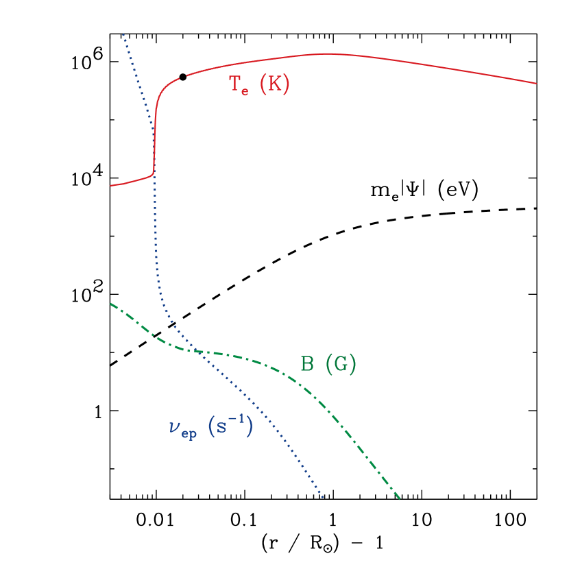
Figure 1.— Radial dependence of plasma parameters from the Cranmer et al. (2007) coronal hole model, including $T_{e}$ (red solid curve), $B$ (green dot-dashed curve), $m_{e}|\Psi|$ (black dashed curve), and $\nu_{ep}$ (blue dotted curve).

In order to use these electron properties as inputs to the Scudder & Olbert (1979) model, the radial variation of the charge-separation electric field must be computed. The electron momentum conservation equation allows us to estimate the gradient of the electric potential $\Phi$ (Jockers, 1970; Hollweg, 1970), with

$$e\frac{\partial\Phi}{\partial r}\,=\,\frac{1}{n_{e}}\frac{\partial}{\partial r}\left(n_{e}k_{\rm B}T_{e\parallel}\right)+\frac{1}{B}\frac{\partial B}{\partial r}k_{\rm B}\left(T_{e\perp}-T_{e\parallel}\right)\,\,,$$ (1)

and this is simplified by assuming $T_{e\parallel}=T_{e\perp}=T_{e}$. Equation (1) is integrated numerically to obtain $\Phi(r)$. The electric potential combines with gravity to give the total potential felt by collisionless electrons,

$$\Psi\,=\,-2\left(\frac{GM_{\odot}}{r}+\ \frac{e\Phi}{m_{e}}\right)$$ (2)

and energy conservation is equivalent to the assumption that the quantity $v_{\parallel}^{2}+v_{\perp}^{2}+\Psi$ remains constant along an electron’s trajectory. In combination with magnetic moment conservation ($v_{\perp}^{2}/B=\mbox{constant}$), this specifies the full “history” of an electron that ends up at a given radius $r$ with known velocity components $v_{\parallel}$ and $v_{\perp}$. Figure 1 shows the radial dependence of $m_{e}|\Psi|$, which is in units of potential energy (eV) and has been normalized to zero at the lower boundary of the model.

The Scudder & Olbert (1979) model is used to compute an iterated electron VDF $f(v_{\parallel},v_{\perp})$ at a test radius $r_{0}$ under the assumption that the VDF at all other radii is given by the local Maxwellian $f_{\rm M}$. For each point in a two-dimensional velocity-space grid at $r_{0}$, the conservation of energy and magnetic moment allows us to solve for $v_{\parallel}$ and $v_{\perp}$ at any other radius $r$. Some electrons undergo turning points, and in those cases it is necessary to also evaluate the lowermost and uppermost radii ($r_{\rm L}$ and $r_{\rm U}$, respectively) that are reached by the electron in question. When no turning point exists in a given direction, we set either $r_{\rm L}$ to the lowermost grid zone (1.003 $R_{\odot}$) or $r_{\rm U}$ to the uppermost grid zone (215 $R_{\odot}$) as needed.

Once an electron’s history and bounding radii are known, the Scudder & Olbert (1979) collisional optical depth quantity $S$ can be calculated for all accessible radii $r_{\rm L}\leq r_{0}\leq r_{\rm U}$, with

$$S(r)\,=\,\left|\int_{r_{0}}^{r}\frac{dr^{\prime}}{2\tau(r^{\prime})v_{\parallel}(r^{\prime})}\right|\,\,.$$ (3)

By definition, $S(r_{0})=0$, and it increases monotonically in both directions as one moves away from this evaluation radius. Distant locations at which $S(r)\gg 1$ are collisionally “opaque” and thus unlikely to influence the VDF at $r_{0}$. Equation (3) utilizes the speed-dependent collisional timescale,

$$\frac{1}{\tau}\,=\,\frac{\nu_{ep}\,w_{e}^{3}\,J(w)}{w^{3}}$$ (4)

where $w$ is the electron’s speed in the solar wind frame, $\nu_{ep}$ is the classical Braginskii (1965) electron–proton collision rate, and $J(w)$ is a dimensionless function that describes the onset of Coulomb runaway for $w\gtrsim w_{e}$ (see Equation (10) of Scudder & Olbert, 1979). Figure 1 shows the radial dependence of $\nu_{ep}$ to illustrate the rapid loss of collisionality in the low corona.

Note that the explicit radial dependence given for many of the above quantities conceals the fact that there is an implicit dependence on the full velocity-space trajectory of the electron in question. In other words, quantities like $\tau(r)$ and $S(r)$ should be specified more precisely as, e.g., $\tau[v_{\parallel}(r,r_{0}),v_{\perp}(r,r_{0})]$, and these functional dependences are unique to each “starting point” in velocity space. The optical depth $S(r)$ is a key ingredient in the analogue of the formal solution to the equation of radiative transfer, which Scudder & Olbert (1979) express as

$$f(r_{0})\,=\,p_{\rm L}\left(f_{\rm M}(r_{\rm L})e^{-S(r_{\rm L})}+\int_{r_{\rm L}}^{r_{0}}dr\,\frac{f_{\rm M}(r)e^{-S(r)}}{\tau(r)v_{\parallel}(r)}\right)$$

$$+\,p_{\rm U}\left(f_{\rm M}(r_{\rm U})e^{-S(r_{\rm U})}+\int_{r_{0}}^{r_{\rm U}}dr\,\frac{f_{\rm M}(r)e^{-S(r)}}{\tau(r)v_{\parallel}(r)}\right)\,\,.$$ (5)

Scudder & Olbert (1979) derived values for the collisional probability factors $p_{\rm L}$ and $p_{\rm U}$ that are different for the upward and downward propagating halves of the VDF. For $v_{\parallel}>0$, $p_{\rm L}=6/7$ and $p_{\rm U}=1/7$. For $v_{\parallel}<0$, $p_{\rm L}=1/7$ and $p_{\rm U}=6/7$. The use of these values results in an unphysical discontinuity at $v_{\parallel}=0$, but it remains a useful first attempt at taking account of the diffusive nature of collisional transport.

Figure 2 shows an example calculation of $f(v_{\parallel},v_{\perp})$ at $r_{0}=1.02\,R_{\odot}$. This height, not far above the transition region, is representative of the location at which the freezing-in of the O⁺⁷/O⁺⁶ ratio is expected to occur. The numerical grid in velocity space was chosen to have 200 points in $v_{\parallel}$ and 100 points in $v_{\perp}$. In radial distance, the Cranmer et al. (2007) coronal hole model was interpolated onto a finer grid of 93,000 points distributed logarithmically between $r=1.003\,R_{\odot}$ and 1 AU. With such a fine grid, the integrals in Equations (3) and (5) converged well with only first-order Eulerian quadrature steps.

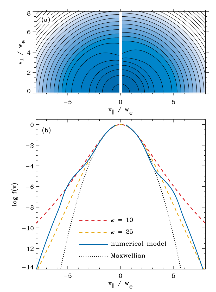
Figure 2.— (a) Contours of constant $f(v_{\parallel},v_{\perp})$ for the test model at $r_{0}=1.02\,R_{\odot}$, with velocity coordinates expressed in units of the local thermal speed $w_{e}$. VDF contours are separated by constant factors of 1 in $\log f$. (b) Slice of $f(v_{\parallel},v_{\perp})$ along the $v_{\perp}=0$ axis (blue solid curve), compared with the local Maxwellian $f_{\rm M}$ (black dotted curve) and two kappa distributions computed with $\kappa=10$ (red dashed curve) and $\kappa=25$ (gold dashed curve).

The discontinuity between the $v_{\parallel}>0$ and $v_{\parallel}<0$ regions of velocity space can be seen most acutely in the mild suprathermal wings ($v\sim 5w_{e}$) that arise because of downward heat transport from the hotter peak temperature at $r\approx 2\,R_{\odot}$. The VDF for downward flowing electrons is enhanced relative to that for upward flowing electrons because of this same heat transport effect. The suprathermal enhancement is reminiscent of the hot “halo” seen at 1 AU (Feldman et al., 1975), which is similarly believed to be the result of nonlocal transport away from the peak temperature region. At $r_{0}$, only a small fraction of the total number of electrons participate in this hot component because the outer corona is somewhat “optically thick” in most parts of velocity space.

For comparison, Figure 2(b) also shows two realizations of the so-called kappa, or generalized Lorentzian distribution,

$$f_{\kappa}(v)\,\propto\,\left[1+\frac{v^{2}}{(\kappa-3/2)w_{e}^{2}}\right]^{-1-\kappa}$$ (6)

(for alternate definitions, see also Vasyliunas, 1968; Cranmer, 1998; Pierrard & Lazar, 2010). No single value of $\kappa$ fits the numerically computed VDF, but the two values of $\kappa=10$ and 25 appear to bracket most of the suprathermal enhancement at $r_{0}$.

Note that the suprathermal VDF shown above was obtained from the fastest wind-speed (and lowest density) model of Cranmer et al. (2007). To assess the applicability of this result to other solar wind conditions, we also computed another set of VDFs using the slowest wind-speed (and highest density) model of Cranmer et al. (2007), corresponding to an active-region streamer. Because this model has a larger transition region height than the polar coronal hole model (see Figure 17 of Cranmer et al., 2007), we computed the Scudder & Olbert (1979) model at a correspondingly larger radius of $r_{0}=1.03\,R_{\odot}$. The resulting VDF exhibits a slightly stronger downward-conducting “shoulder” at $v_{\parallel}/w_{e}\approx-4$ and a slightly less intense tail at $|v_{\parallel}/w_{e}|\gtrsim 6$, but most of the suprathermal electrons still fall between the $\kappa=10$ and 25 curves.

3. Frozen-In Ionization Fractions at 1 AU

Owocki & Scudder (1983) and Bürgi (1987) first studied the possibility that suprathermal electrons in the corona may enhance the frozen-in ion charge state ratios measured at 1 AU. Later, when it was found that the freezing-in temperatures are anticorrelated with wind speed (e.g., von Steiger et al., 2000), it was realized that these nonequilibrium ionization processes could be key diagnostics of the physical processes responsible for solar wind acceleration. Thus, in order to better test the MHD turbulence paradigm used in the Cranmer et al. (2007) models, we want to estimate the O⁺⁷/O⁺⁶ ionization fraction ratios that would be consistent with the suprathermal VDFs described above.

Figure 15 of Cranmer et al. (2007) showed the wind speed dependence of the modeled O⁺⁷/O⁺⁶ fraction at 1 AU for a series of 18 open flux-tube models of coronal holes, quiescent equatorial streamers, and active-region streamers. The original nonequilibrium ionization calculations assumed that the coronal electron VDFs remained perfectly Maxwellian. For this paper, a representative freezing-in radius was determined—in each of these 18 models—by finding the location at which local ionization equilibrium would have given the same O⁺⁷/O⁺⁶ ratio as in the full nonequilibrium model. The temperature $T_{f}$ at this radius was then assumed to be that model’s core freezing-in temperature, and $T_{f}$ was used when looking up the ionization fractions from tables computed with varying $\kappa$ exponents. We used the tabulated ionization balance calculations of Dzifčáková & Dudík (2013), which included collisional ionization, autoionization, radiative recombination, and dielectronic recombination. This process was also repeated using the earlier kappa-dependent ionization balance data from Wannawichian et al. (2003), and the results were the same.

Figure 3(a) shows a subset of the equilibrium O⁺⁷/O⁺⁶ ratios from Dzifčáková & Dudík (2013), and Figure 3(b) shows how these map onto the open flux-tube models of Cranmer et al. (2007). The corresponding ionization fractions for Maxwellian VDFs were taken from version 7.1 of the CHIANTI database (Dere et al., 1997; Landi et al., 2013). The observational data are the same statistical summaries of Ulysses SWICS (Solar Wind Ion Composition Spectrometer; Gloeckler et al., 1992) measurements that were presented by Cranmer et al. (2007). The model with $\kappa=10$ clearly matches the SWICS data better than the Maxwellian model. Figure 2(b) above indicates that this degree of suprathermal electron enhancement agrees reasonably well with (at least the down-conducted half of) what the Scudder & Olbert (1979) transport model predicts should exist at the freezing-in height.

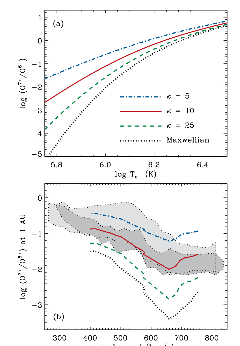
Figure 3.— Ratio of O⁷⁺ to O⁶⁺ number densities plotted versus (a) equilibrium $T_{e}$, and (b) solar wind speed at 1 AU for the standard set of Cranmer et al. (2007) models. Line styles (consistent in both panels) denote assumed VDF shapes. Binned Ulysses data from 1990–1994 solar maximum (light gray region) and 1994–1995 fast latitude scan (dark gray region) are shown for comparison.

4. Discussion and Conclusions

It has sometimes been asserted (e.g., Antiochos et al., 2011) that the striking differences in ion composition between fast and slow streams is evidence that the two types of solar wind cannot be driven by the same physical process. However, the wave/turbulence model of Cranmer et al. (2007) serves as one counterexample, in which the observed trends in the O⁺⁷/O⁺⁶ and Fe/O (elemental abundance) ratios versus wind speed are a natural by-product of a single mechanism operating in differently shaped magnetic flux tubes. These models utilize identical photospheric lower boundary conditions, but their variable rates of coronal heating depend on the magnetic field via the reflection and cascade of Alfvén waves. Conduction from the corona to the transition region carries this “information” back down to the heights at which different rates of ionization and elemental fractionation occur. This letter’s refined model of suprathermal electron production and nonequilibrium ionization shows that the wave/turbulence model can explain not only the observed wind-speed trends, but also the absolute values of the O⁺⁷/O⁺⁶ ratios.

Despite these successes, there is still uncertainty about the ability of a single type of solar wind heating mechanism to explain the full range of observed ion composition effects in the heliosphere. For example, the slow wind from unipolar pseudostreamers appears to defy the well-known empirical anticorrelation between wind speed and superradial flux-tube expansion (Wang et al., 2012). Models that employ specific physical processes need to be constructed for global, three-dimensional descriptions of the heliosphere (e.g., van der Holst et al., 2014; Usmanov et al., 2014) at times when the coronal and heliospheric plasma state is well-observed.

Future work must also involve more physical realism for the models of suprathermal electron transport and nonequilibrium ionization. The Scudder & Olbert (1979) model used above was applied only for a single iterative step of refinement away from an assumed Maxwellian VDF in the regions surrounding the test radius $r_{0}$. It is suspected that the strength of the suprathermal tails may be enhanced as a result of iterating multiple times to a self-consistent set of VDFs over a range of coronal radii. Improved techniques of describing weakly collisional particle transport (e.g., solving Fokker-Planck type equations) have been successful in modeling various suprathermal electron effects in the corona and solar wind (e.g., Lie-Svendsen & Leer, 2000; Vocks et al., 2008; Smith et al., 2012). A full set of nonequilibrium, non-Maxwellian ionization balance calculations should also be performed for all of the ions with number densities measured in interplanetary space, not just O⁺⁷ and O⁺⁶ (see Landi et al., 2012a).

References

- Anderson et al. (1996) Anderson, S. W., Raymond, J. C., & van Ballegooijen, A. 1996, ApJ, 457, 939
- Antiochos et al. (2011) Antiochos, S. K., Mikić, Z., Titov, V., Lionello, R., & Linker, J. 2011, ApJ, 731, 112
- Braginskii (1965) Braginskii, S. I. 1965, Rev. Plasma Phys., 1, 205
- Bürgi (1987) Bürgi, A. 1987, J. Geophys. Res., 92, 1057
- Cranmer (1998) Cranmer, S. R. 1998, ApJ, 508, 925
- Cranmer (2009) Cranmer, S. R. 2009, Living Rev. Solar Phys., 6, 3
- Cranmer et al. (2007) Cranmer, S. R., van Ballegooijen, A. A., & Edgar, R. J. 2007, ApJS, 171, 520
- Dere et al. (1997) Dere, K. P., Landi, E., Mason, H. E., et al. 1997, A&AS, 125, 149
- Dzifčáková & Dudík (2013) Dzifčáková, E., & Dudík, J. 2013, ApJS, 206, 6
- Esser & Edgar (2000) Esser, R., & Edgar, R. J. 2000, ApJ, 532, L71
- Esser & Edgar (2001) Esser, R., & Edgar, R. J. 2001, ApJ, 563, 1055
- Feldman et al. (1975) Feldman, W. C., Asbridge, J. R., Bame, S. J., et al. 1975, J. Geophys. Res., 80, 4181
- Feng et al. (2012) Feng, L., Inhester, B., de Patoul, J., et al. 2012, A&A, 538, A34
- Geiss et al. (1995) Geiss, J., Gloeckler, G., & von Steiger, R. 1995, Space Sci. Rev., 72, 49
- Gloeckler et al. (1992) Gloeckler, G., Geiss, J., Balsiger, H., et al. 1992, A&AS, 92, 267
- Hollweg (1970) Hollweg, J. V. 1970, J. Geophys. Res., 75, 2403
- Hundhausen et al. (1968) Hundhausen, A. J., Gilbert, H. E., & Bame, S. J. 1968, ApJ, 152, L3
- Jockers (1970) Jockers, K. 1970, A&A, 6, 219
- Ko et al. (1997) Ko, Y.-K., Fisk, L. A., Geiss, J., et al. 1997, Sol. Phys., 171, 345
- Ko et al. (1996) Ko, Y.-K., Fisk, L. A., Gloeckler, G., et al. 1996, Geophys. Res. Lett., 23, 2785
- Ko et al. (2014) Ko, Y.-K., Muglach, K., Wang, Y.-M., et al. 2014, ApJ, 787, 121
- Kulinová et al. (2011) Kulinová, A., Kašparová, Dzifčáková, E., et al. 2011, A&A, 533, A81
- Landi et al. (2012a) Landi, E., Alexander, R. L., Gruesbeck, J. R., et al. 2012a, ApJ, 744, 100
- Landi et al. (2012b) Landi, E., Gruesbeck, J. R., Lepri, S. T., et al. 2012b, ApJ, 750, 159
- Landi et al. (2013) Landi, E., Young, P. R., Dere, K. P., et al. 2013, ApJ, 763, 86
- Levine (1974) Levine, R. H. 1974, ApJ, 190, 457
- Lie-Svendsen & Leer (2000) Lie-Svendsen, Ø., & Leer, E. 2000, J. Geophys. Res., 105, 35
- Marsch (2006) Marsch, E. 2006, Living Rev. Solar Phys., 3, 1
- Ogilvie & Scudder (1978) Ogilvie, K. W., & Scudder, J. D. 1978, J. Geophys. Res., 83, 3776
- Owocki et al. (1983) Owocki, S. P., Holzer, T. E., & Hundhausen, A. J. 1983, ApJ, 275, 354
- Owocki & Scudder (1983) Owocki, S. P., & Scudder, J. D. 1983, ApJ, 270, 758
- Parker (1958a) Parker, E. N. 1958a, ApJ, 128, 664
- Parker (1958b) Parker, E. N. 1958b, ApJ, 128, 677
- Parnell & De Moortel (2012) Parnell, C. E., & De Moortel, I. 2012, Phil. Trans. Roy. Soc. A, 370, 3217
- Pierrard & Lazar (2010) Pierrard, V., & Lazar, M. 2010, Sol. Phys., 267, 153
- Ralchenko et al. (2007) Ralchenko, Y., Feldman, U., & Doschek, G. A. 2007, ApJ, 659, 1682
- Roberts & Miller (1998) Roberts, D. A., & Miller, J. A. 1998, Geophys. Res. Lett., 25, 607
- Scudder (1992) Scudder, J. D. 1992, ApJ, 398, 319
- Scudder & Olbert (1979) Scudder, J. D., & Olbert, S. 1979, J. Geophys. Res., 84, 2755
- Smith et al. (2012) Smith, H. M., Marsch, E., & Helander, P. 2012, ApJ, 753, 31
- Usmanov et al. (2014) Usmanov, A. V., Goldstein, M. L., & Matthaeus, W. H. 2014, ApJ, 788, 43
- van der Holst et al. (2014) van der Holst, B., Sokolov, I. V., Meng, X., et al. 2014, ApJ, 782, 81
- Vasyliunas (1968) Vasyliunas, V. M. 1968, J. Geophys. Res., 73, 2839
- Viñas et al. (2000) Viñas, A. F., Wong, H. K., & Klimas, A. J. 2000, ApJ, 528, 509
- Vocks et al. (2008) Vocks, C., Mann, G., & Rausche, G. 2008, A&A, 480, 527
- von Steiger et al. (2000) von Steiger, R., Schwadron, N. A., Fisk, L. A., et al. 2000, J. Geophys. Res., 105, 27217
- Wang et al. (2012) Wang, Y.-M., Grappin, R., Robbrecht, E., et al. 2012, ApJ, 749, 182
- Wannawichian et al. (2003) Wannawichian, S., Ruffolo, D., & Kartavykh, Y. Y. 2003, ApJS, 146, 443
- Yoon et al. (2006) Yoon, P. H., Rhee, T., & Ryu, C.-M. 2006, J. Geophys. Res., 111, A09106