Observation of antiferromagnetic correlations in the Hubbard model with ultracold atoms
Abstract
Ultracold atoms in optical lattices have great potential to contribute to a better understanding of some of the most important issues in many-body physics, such as high-temperature (high-) superconductivity PhysRevLett.89.220407 . Thirty years ago, Anderson suggested that the Hubbard model, a simplified representation of fermions moving on a periodic lattice, may contain the essence of copper oxide superconductivity ANDERSON87 . The Hubbard model describes many of the features shared by the copper oxides, including an interaction-driven Mott insulating state and an antiferromagnetic (AFM) state. Optical lattices filled with a two-spin-component Fermi gas of ultracold atoms can faithfully realise the Hubbard model with readily tunable parameters, and thus provide a platform for the systematic exploration of its phase diagram Jaksch2005 ; Bloch2008 . Realisation of strongly correlated phases, however, has been hindered by the need to cool the atoms to temperatures as low as the magnetic exchange energy, and also by the lack of reliable thermometry McKay2011 . Here we demonstrate spin-sensitive Bragg scattering of light to measure AFM spin correlations in a realisation of the three-dimensional (3D) Hubbard model at temperatures down to 1.4 times that of the AFM phase transition. This temperature regime is beyond the range of validity of a simple high-temperature series expansion, which brings our experiment close to the limit of the capabilities of current numerical techniques. We reach these low temperatures using a unique compensated optical lattice technique Mathy2012 , in which the confinement of each lattice beam is compensated by a blue-detuned laser beam. The temperature of the atoms in the lattice is deduced by comparing the light scattering to determinantal quantum Monte Carlo Blankenbecler1981 (DQMC) and numerical linked-cluster expansion Rigol2006 (NLCE) calculations. Further refinement of the compensated lattice may produce even lower temperatures which, along with light scattering thermometry, would open avenues for achieving and characterising other novel quantum states of matter, such as the pseudogap regime of the 2D Hubbard model.
A two-spin-component Fermi gas in a simple cubic optical lattice may be described by a single-band Hubbard model with nearest-neighbour tunnelling and on-site interaction . At a density of one atom per site, and for sufficiently large there is a crossover from a ‘metallic’ state to a Mott insulating regime RevModPhys.70.1039 as the temperature is reduced below . The Mott regime has been demonstrated with ultracold atoms in an optical lattice by observing the reduction of doubly occupied sites Jordens2008 and the related reduction of the global compressibility Schneider2008 . For below the Néel ordering temperature , which for is approximately equal to the exchange energy , the system undergoes a phase transition to an AFM state Staudt2000 . In the context of quantum simulations, AFM phases of Ising spins have been previously engineered with bosonic atoms in an optical lattice Simon2011 and with spin- ions Kim2010 ; Britton2012 . Also, nearest-neighbour AFM correlations due to magnetic exchange have been observed along one dimension of an anisotropic lattice Greif2013 . The same experiment achieved temperatures as low as when the lattice was configured to be isotropic Imriska2014 , where is the maximal value of the Néel transition temperature Staudt2000 ; Paiva2011 ; Kozik2013 .
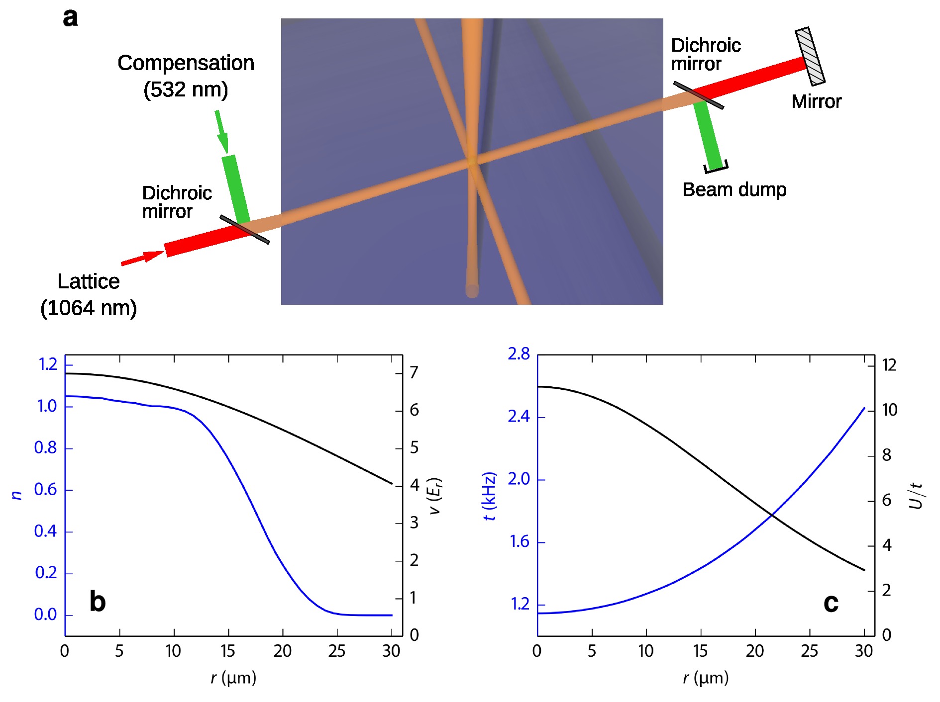
Our experiments are performed with an all-optically produced Duarte2011 , quantum degenerate, two-state mixture of the two lowest hyperfine ground states of fermionic 6Li atoms, which we label and . The repulsive interaction between atoms in states and is controlled via a magnetic Feshbach resonance Houbiers1998 , which we use to set the -wave scattering length in the range from 80 to 560 , where is the Bohr radius. A simple cubic optical lattice is formed at the intersection of three mutually perpendicular infrared (IR) retroreflected laser beams. We can dynamically rotate the polarisation of the retroreflection, and thus continually adjust the potential between a lattice and a harmonic dimple trap. The overall confinement produced by the Gaussian envelope of each IR lattice beam is partially compensated with a superimposed, non-retroreflected, blue-detuned laser beam Ma2008 ; Mathy2012 . The compensation beams serve three purposes: (1) They help flatten the confining potential in order to enlarge the volume of the AFM phase; (2) they provide a way to maintain the central density near as the lattice is loaded; and (3) they may mitigate the effects of heating in the lattice by lowering the threshold for evaporation.
A degenerate sample with total atom number between and is prepared in the harmonic dimple trap (without compensation) at a temperature , where is the Fermi temperature. The lattice is turned on slowly to a central depth of (see Methods), where is the recoil energy, is Planck’s constant, is the atomic mass, and is the wavelength of the lattice beams. While loading the lattice, the intensities of the compensation beams are adjusted to maintain a peak density . We have measured the temperature in the dimple trap before and after transferring the atoms to the lattice (see Methods and Extended Data Fig. 3), and have observed that the compensating beams mitigate heating in the lattice, perhaps by allowing continued evaporative cooling Mathy2012 or by a reduction of three-body loss.
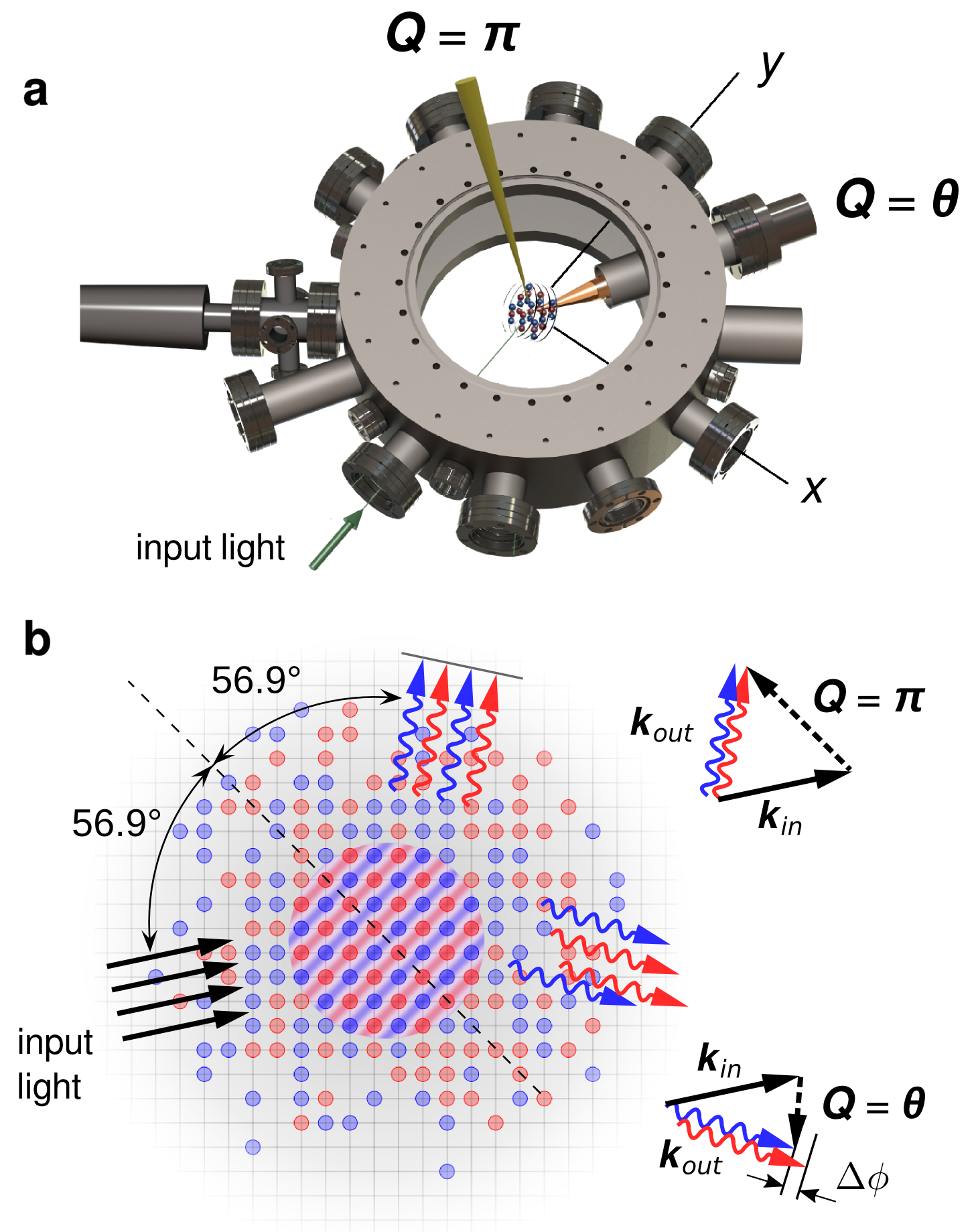
Bragg scattering of near-resonant light Birkl1995 ; Weidemueller1998 ; Miyake2011 is depicted in Fig. 1. The Bragg condition for scattering from an AFM ordered sample is satisfied when the momentum transferred to a scattered photon is equal to , where is a reciprocal lattice vector of the magnetic sublattice, and is the lattice spacing. Cameras are positioned to detect scattering at and also at , a momentum transfer that does not satisfy the Bragg condition and is used as a control. We obtain spin sensitivity, in analogy to neutron scattering in condensed matter, by setting the Bragg laser frequency between the optical transition frequencies for the two spin states Corcovilos2010 ; Werner2005 . Prior to the measurement, we jump to in a few to lock the atoms in place (see Methods), and then illuminate them in-situ for with the Bragg probe. Alternatively, we can suddenly turn off the lattice and illuminate the atoms after time-of-flight .
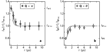
Figure 2 shows the results of simultaneous measurements of the scattered intensity for and ( and , respectively), as a function of . After a few of expansion, when the extent of the atomic wavepackets becomes comparable to the lattice spacing, the light scattered from correlated spins no longer interferes constructively at the detector. More precisely, the Debye-Waller factor decays to zero after a sufficiently long (see Methods) and the sample is effectively uncorrelated. Here is the displacement of an atom from the centre of the lattice site at which it was initially localised.
By comparing the intensity of the light scattered in-situ () to that after sufficiently long ( and , respectively), we effectively normalise the Bragg scattering signal to the diffuse scattering background of an uncorrelated sample, achieving high sensitivity to magnetic ordering and strong rejection of common mode systematics. Figure 2 shows that there is enhanced scattering at relative to the uncorrelated cloud () for , whereas for scattering at is reduced, such that . Double occupancies, present as ‘virtual’ states even at low temperatures Fuchs2011 , reduce coherent scattering in all directions, since each atom in the pair has opposite spin and therefore scatters with opposite phase. For the coherent enhancement from AFM spin correlations exceeds this reduction. Furthermore, the coherent enhancement of the signal along suppresses the scattered intensity in other directions.
For a momentum transfer , the spin structure factor of the sample is defined as
| (1) |
Here is the total number of atoms, the sums extend over all lattice sites and , is the location of the site, and is the component of the spin operator for the site:
In a sample with complete AFM ordering , whereas for uncorrelated samples in the lattice and . The choice of the spin component for this analysis is arbitrary, as each of the other axes would result in the same value for in the absence of a symmetry-breaking field. In the limit of tightly localised wavefunctions (), and for a weak probe, the spin structure factor is . We determine the spin structure factor by measuring the scattered intensities and and applying a correction to account for the in-situ Debye-Waller factor in the 20 lattice and for saturation of the atomic transition, which generates a small component of inelastically scattered light (see Methods).
Within the local density approximation (LDA) we model the sample by considering each point in the trap as a homogeneous system in equilibrium at a temperature , with local values of the chemical potential and the Hubbard parameters determined by the trap potential. The spin structure factor of the sample can then be expressed as the integral over the trap of the local spin structure factor per lattice site, . Figure 3a shows numerical calculations of for various temperatures in a homogeneous lattice with , close to where is maximal Staudt2000 . The figure shows that is sharply peaked around and grows rapidly as approaches from above.
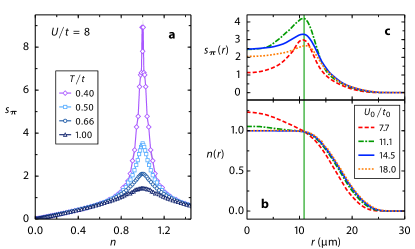
Figures 3b and 3c show and profiles, respectively, calculated for our experimental parameters at various values of , where and denote the local values of the Hubbard parameters at the centre of the trap. As seen in Fig. 3b, only a fraction of the atoms in the sample is near , where AFM correlations are maximal. The finite extent of the lattice beams causes the lattice depth to decrease with distance from the centre, resulting in an increasing such that both and decrease with increasing radius for constant (see Extended Data Fig. 1). The radial decrease in causes to maximise at the largest radius for which the density is . For large the cloud exhibits an Mott plateau and is maximised at the outermost radius of the plateau.
In the experiment, we measure as a function of . At each value of we vary the atom number to maximise the measured (see Methods and Extended Data Fig. 2). According to the picture presented above, this has the effect of optimising the size and location of the region of the cloud such that AFM correlations are maximised. The compensation strength , which is the same for all , was also adjusted to maximise . We found the optimum to be at a lattice depth (see Methods). Besides the equilibrium considerations regarding the optimal size and location of the Mott plateau, we believe that the dynamical adjustment of during the lattice turn-on reduces the time for the system to equilibrate, by minimising the deviation of the equilibrium density distribution in the final potential from the starting density distribution in the dimple trap prior to loading the lattice.
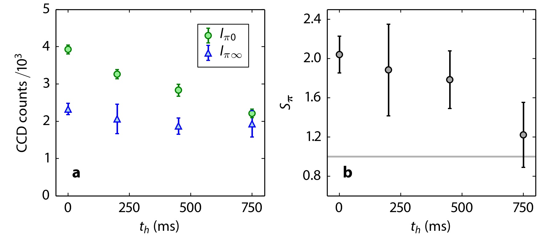
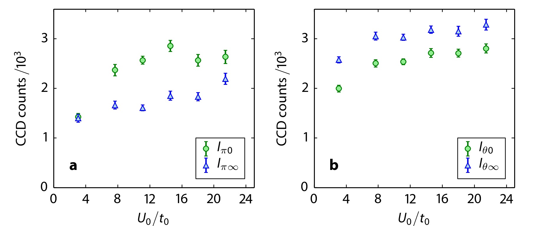
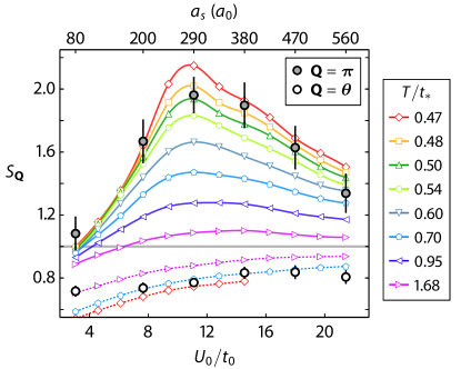
Figure 4 shows the measured values of and at optimal for various values of (see Extended Data Fig. 5 for the raw counts at the CCD cameras). We find that is peaked for . In contrast, the measurements of vary little over the range of interaction strengths, consistent with an absence of coherent Bragg scattering in this direction. Measurements of after hold time in the lattice show that the Bragg signal decays for larger temperatures (see Extended Data Fig. 4). Comparing the measured with numerical calculations for a homogeneous lattice (for example, those in Fig. 3a) allows us to set a trap independent upper limit on the temperature, which we determine to be .
Precise thermometry is obtained by comparing the measured with numerical calculations averaged over the trap density distribution for different values of . The results of such numerical calculations are shown in Fig. 4, labelled by the value of , which we define as the local value of at the radius where the spin structure factor per lattice site is maximal (see Fig. 3c). At , where measured AFM correlations are maximal, we find , where the uncertainty is due to the statistical error in the measured and the systematic uncertainty in the lattice parameters used for the numerical calculation. This temperature is consistent with the data at all values of . We caution, however, that for values of a single-band Hubbard model may not be adequate, as corrections involving higher bands may become non-negligible Werner2005 ; Mathy2009 .
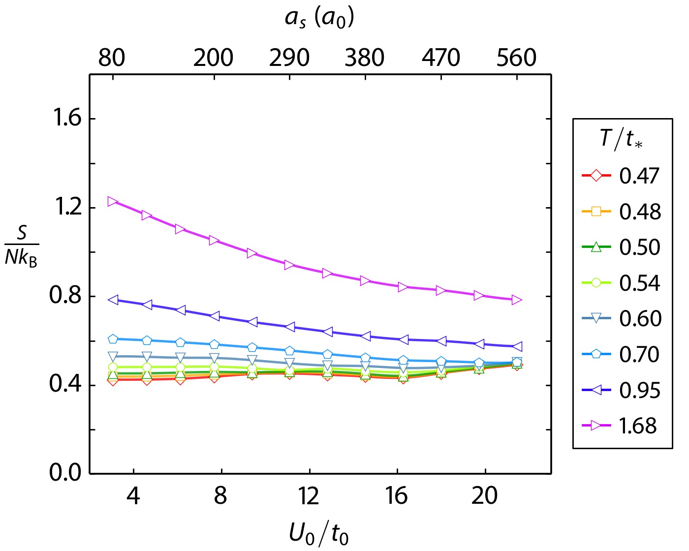
As was shown in Fig. 3b, for the dominant contribution to comes from the outermost radius of the Mott plateau. At that radius, the local value of is , consistent with DQMC calculations for the homogeneous lattice Staudt2000 ; Paiva2011 ; Kozik2013 , which find to be maximised for between 8 and 9. For , , so we can infer the temperature of the system to be . In terms of , the temperature is . At this temperature, the numerical calculations indicate that the correlation length is approximately the lattice spacing. The calculations show that the entropy per particle in the trap is , where is the Boltzmann constant (see Extended Data Fig. 6). This entropy range is consistent with measured in the harmonic dimple trap before loading the atoms into the lattice Kohl2006 , and thus justifies the assumption of adiabatic loading.
In conclusion, we have observed AFM correlations in the 3D Hubbard model using ultracold atoms in an optical lattice via spin-sensitive Bragg scattering of light. Because magnetic order is extremely sensitive to in the vicinity of , Bragg scattering provides precise thermometry in regimes previously inaccessible to quantitative temperature measurements. While previous cold atom experiments on the 3D Fermi-Hubbard model were in a temperature regime that could be accurately represented by a simple high-temperature series expansion, the data presented here is near the limit of the capabilities of advanced numerical simulations. Our experimental setup can be configured to study the 2D Hubbard model in an array of planes; further progress to lower temperature will put us in a position to answer questions about competing pairing mechanisms in 2D, and may ultimately resolve the long standing question of d-wave superconductivity in the Hubbard model.
References
- (1) W. Hofstetter, J. I. Cirac, P. Zoller, E. Demler, and M. D. Lukin, Phys. Rev. Lett. 89, 220407 (2002).
- (2) P. W. Anderson, Science 235, 1196 (1987).
- (3) D. Jaksch and P. Zoller, Annals of Physics 315, 52 (2005), special Issue.
- (4) I. Bloch, J. Dalibard, and W. Zwerger, Rev. Mod. Phys. 80, 885 (2008).
- (5) D. C. McKay and B. DeMarco, Reports on Progress in Physics 74, 054401 (2011).
- (6) C. J. M. Mathy, D. A. Huse, and R. G. Hulet, Phys. Rev. A 86, 023606 (2012).
- (7) R. Blankenbecler, D. J. Scalapino, and R. L. Sugar, Phys. Rev. D 24, 2278 (1981).
- (8) M. Rigol, T. Bryant, and R. R. P. Singh, Phys. Rev. Lett. 97, 187202 (2006).
- (9) M. Imada, A. Fujimori, and Y. Tokura, Rev. Mod. Phys. 70, 1039 (1998).
- (10) R. Jördens, N. Strohmaier, K. Günter, H. Moritz, and T. Esslinger, Nature 455, 204 (2008).
- (11) U. Schneider, L. Hackermüller, S. Will, T. Best, I. Bloch, T. A. Costi, R. W. Helmes, D. Rasch, and A. Rosch, Science 322, 1520 (2008).
- (12) R. Staudt, M. Dzierzawa, and A. Muramatsu, The European Physical Journal B - Condensed Matter and Complex Systems 17, 411 (2000).
- (13) J. Simon, W. S. Bakr, R. Ma, M. E. Tai, P. M. Preiss, and M. Greiner, Nature 472, 307 (2011).
- (14) K. Kim, M.-S. Chang, S. Korenblit, R. Islam, E. Edwards, J. Freericks, G.-D. Lin, L.-M. Duan, and C. Monroe, Nature 465, 590 (2010).
- (15) J. W. Britton, B. C. Sawyer, A. C. Keith, C.-C. J. Wang, J. K. Freericks, H. Uys, M. J. Biercuk, and J. J. Bollinger, Nature 484, 489 (2012).
- (16) D. Greif, T. Uehlinger, G. Jotzu, L. Tarruell, and T. Esslinger, Science 340, 1307 (2013).
- (17) J. Imriška, M. Iazzi, L. Wang, E. Gull, D. Greif, T. Uehlinger, G. Jotzu, L. Tarruell, T. Esslinger, and M. Troyer, Phys. Rev. Lett. 112, 115301 (2014).
- (18) T. Paiva, Y. L. Loh, M. Randeria, R. T. Scalettar, and N. Trivedi, Phys. Rev. Lett. 107, 086401 (2011).
- (19) E. Kozik, E. Burovski, V. W. Scarola, and M. Troyer, Phys. Rev. B 87, 205102 (2013).
- (20) P. M. Duarte, R. A. Hart, J. M. Hitchcock, T. A. Corcovilos, T.-L. Yang, A. Reed, and R. G. Hulet, Phys. Rev. A 84, 061406 (2011).
- (21) M. Houbiers, H. T. C. Stoof, W. I. McAlexander, and R. G. Hulet, Phys. Rev. A 57, R1497 (1998).
- (22) P. N. Ma, K. Y. Yang, L. Pollet, J. V. Porto, M. Troyer, and F. C. Zhang, Phys. Rev. A 78, 023605 (2008).
- (23) G. Birkl, M. Gatzke, I. H. Deutsch, S. L. Rolston, and W. D. Phillips, Phys. Rev. Lett. 75, 2823 (1995).
- (24) M. Weidemüller, A. Görlitz, T. W. Hänsch, and A. Hemmerich, Phys. Rev. A 58, 4647 (1998).
- (25) H. Miyake, G. A. Siviloglou, G. Puentes, D. E. Pritchard, W. Ketterle, and D. M. Weld, Phys. Rev. Lett. 107, 175302 (2011).
- (26) T. A. Corcovilos, S. K. Baur, J. M. Hitchcock, E. J. Mueller, and R. G. Hulet, Phys. Rev. A 81, 013415 (2010).
- (27) F. Werner, O. Parcollet, A. Georges, and S. R. Hassan, Phys. Rev. Lett. 95, 056401 (2005).
- (28) S. Fuchs, E. Gull, L. Pollet, E. Burovski, E. Kozik, T. Pruschke, and M. Troyer, Phys. Rev. Lett. 106, 030401 (2011).
- (29) C. J. M. Mathy and D. A. Huse, Phys. Rev. A 79, 063412 (2009).
- (30) M. Köhl, Physical Review A 73, 031601 (2006).
I Acknowledgements
This work was supported under ARO Grant No. W911NF-13-1-0018 with funds from the DARPA OLE program, NSF, ONR, the Welch Foundation (Grant No. C-1133), and an ARO-MURI grant No. W911NF-14-1-003. T.P. acknowledges support from CNPq, FAPERJ, and the INCT on Quantum Information. RTS acknowledges support from the Office of the President of the University of California.
II Author Contributions
The experimental work was performed by R.A.H., P.M.D., T.-L.Y., X.L., and R.G.H., while T.P., E.K., P.M.D., R.T.S., N.T., and D.A.H. performed the theory needed to extract temperatures from the data and provided overall theoretical guidance. All authors contributed to the writing of the manuscript. *
Appendix A METHODS
A.1 Preparation.
6Li atoms are first captured and cooled in a magneto-optical trap (MOT) operating at 671 nm. They are further cooled in a second MOT stage employing 323 nm light near resonant with the transition. As described previously Duarte2011 , these atoms are laser cooled into a large volume optical dipole trap (ODT) where a balanced spin mixture of the states and is produced.
Once the large volume ODT is loaded, we set the magnetic field to 340 G () to perform evaporative cooling. The intensities of the lattice beams (1,064 nm) in dimple configuration (with the polarisation of each retroreflection perpendicular to that of each input beam) are turned on in 1 s. The depth of the dimple, which at this point is only a small perturbation on the ODT, is adjusted to control the final atom number in the experiment. The depth of the ODT is then ramped to zero in 5.5 s to evaporatively cool the atoms into the dimple. To produce a final sample with repulsive interactions, the magnetic field is increased to 595 G () in a 5 ms linear ramp starting 3 s into the evaporation trajectory. Due to the small volume of the dimple relative to the ODT, evaporation into the dimple is efficient and deeply degenerate samples are reliably produced.
We measure in the dimple trap by fitting the density profile, after 0.5 ms of time-of-flight, to a Thomas-Fermi distribution Butts1997 . The magnetic field is tuned to 528 G to make the gas non-interacting prior to the measurement. For the experiments reported here, the final dimple depths are in the range between and per axis, resulting in between . The measured value is independent of within this range. The uncertainty in is the standard deviation of the fitted value for at least six independent realisations.
A.2 Compensated optical lattice.
The experiment takes place in a compensated simple cubic optical lattice potential that can be expressed as
where
and , are the potentials produced by the lattice (1,064 nm) and compensation (532 nm) beams respectively:
Here, is the lattice depth and is the compensation (). A schematic of the compensated lattice, and the spatial variation of the Hubbard parameters due to the finite lattice beam waists, are shown in Extended Data Fig. 1.
The beam waists ( radius) of the three axes are calibrated independently by phase modulation spectroscopy of each lattice beam and by measuring the frequency of breathing mode oscillations. The waists are found to be (up to a systematic uncertainty) m and m, for beams propagating along , respectively.
A.3 Lattice loading.
To load the lattice from the dimple trap we first rotate the polarisation of the retroreflected beams parallel to that of the input beams in 100 ms. In the following 25 ms, we increase the lattice depth to and ramp the magnetic field to set the final value of . The lattice depth is then ramped to in 15 ms.
Throughout the process of loading the lattice from the dimple, the power of the compensating beams is adjusted in order to maintain the peak density of the sample at . At the final lattice depth of , the average compensation per beam is . The value of for each beam is adjusted slightly from this average in order to create samples that appear spherically symmetric.
A.4 Round-trip measurements.
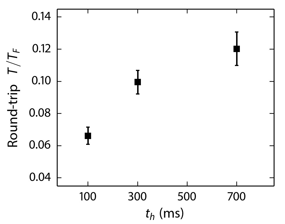
After loading the atoms into the lattice we wait for a hold time and then reverse the lattice loading ramps to return to the harmonic dimple trap and measure . This measurement, shown in Extended Data Fig. 3, sets an upper limit on the entropy of the system in the lattice, and is also a measure of the heating rate of the system in the lattice.
A.5 Temperature dependence of
In Extended Data Fig. 4 we show as a function of hold time in the lattice and observe that it decays for longer hold times, as expected from the increase in . Although the preparation of the sample and the final potential are somewhat different for the data presented in Extended Data Figs. 3 and 4, the data support the contention that the Bragg signal decreases with increasing .
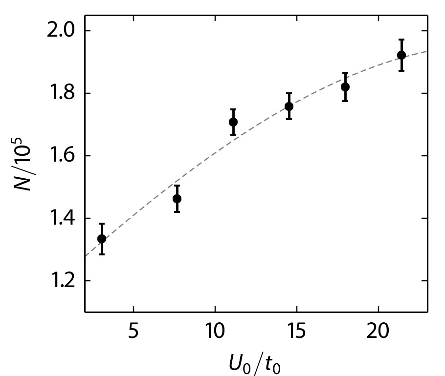
A.6 Variation of to maximise .
The global chemical potential must be increased for larger to guarantee the formation of a Mott plateau in the trap. A larger results in larger atom number. is adjusted to maximise the Bragg signal for each experimental value of in Fig. 4. We adjust by tuning the depth of the dimple trap in which degeneracy is achieved prior to loading the atoms into the lattice. The optimal value of as a function of is shown in Extended Data Fig. 2.
A.7 Spin structure factor measurement.
We measure the spin structure factor at two different values of the momentum transfer given by
where is the lattice spacing.
We detect the scattered light using two separate cameras as the cloud is illuminated with the Bragg probe beam for s. The Bragg probe beam is a collimated Gaussian beam with a waist of m and W of power, resulting in an intensity . The intensity of the probe determines the on-resonance saturation parameter , where is the speed of light, is the polarisation of the probe light, is the unit vector in the direction of the dipole matrix element of the transition, is the wavelength of the transition, and is its linewidth. The polarisation of the incident light in our experiment is linear and perpendicular to the quantisation axis, so . The Bragg probe detuning is set between the two spin states, such that , where and are the detunings from the two spin states.
The spin structure factor is defined in equation (1) as a sum over lattice sites . By quickly ramping the lattice depth to , the state of the system is projected into a product state, where the wavefunction of each atom is localised at a lattice site. Hence, we can write as a sum over particles :
where is the component of the spin of the atom.
When illuminated with the probe light, each atom can be considered as an independent scatterer, and the intensity at the detector can be obtained by summing the field contributions from the individual atoms and squaring the total field. We assume that the spatial wavefunction of all atoms is the harmonic oscillator ground state in a lattice site of depth , and that it does not change during the measurement. The resulting intensity at the detector is given by
| (2) |
where , and . Here is the polarisation vector of the scattered field, , where is a unit vector pointing in the direction of the detector.
In equation (2) the first term arises from uncorrelated scattering by the atoms, while the second term represents the interference due to magnetic correlations. We can identify the spin structure factor in the interference term as
and obtain
where , and the correction factor is . In the experiment we obtain by combining measurements of the scattered intensity in-situ () and after sufficiently long time-of-flight (). The correction factor takes the values for and for .
A.8 Time-of-flight.
After the atoms are released in time-of-flight, the Debye-Waller factor decays as the atomic wavefunctions expand, resulting in a corresponding decay of the Bragg scattered intensity. For a lattice of depth
This equation was used to calculate the solid grey line in Fig. 2. The average value of the Debye-Waller factor during the duration of the Bragg exposure
is used to calculate the dashed grey line in Fig. 2.
The data shown in Fig. 2 was taken at with atoms. This value of is above the optimal value, so the ratio of in Fig. 2 gives , which is less than the expected optimal value of from Fig. 4.
A.9 Momentum transferred from the probe to the atoms.
As mentioned above, we assume that the spatial wavefunction of the atoms remains unchanged for the duration of the exposure. For this assumption to be valid, the Lamb-Dicke parameter needs to be . In the 20 lattice, , meaning that approximately one out of every 4 photons scattered will excite an atom to the second band of the lattice. An atom in the second band has larger position uncertainty and hence a smaller Debye-Waller factor, which reduces its contribution to the Bragg scattering signal.
The total number of photons scattered per atom is given by , where the duration of the probe is s. For and , , thus justifying the assumption that the atoms remain in the lowest band during the pulse.
For the Bragg scattering measurements performed after time-of-flight, the momentum transferred from the probe to the atoms plays a more significant role, since the atoms are not trapped and will recoil after every photon scatter. Despite this, we still see a good agreement between the observed decay of the Bragg scattering signal and the decay expected for a Heisenberg limited wavepacket, as shown in Fig. 1. We have also performed non-spin-sensitive Bragg scattering measurements from the 010 planes of the lattice and observe the same agreement, justifying that momentum transfer from the probe to the atoms can be neglected for the exposure times used.
A.10 Optical density.
A low optical density of the sample is important so that the probe is unattenuated through the atom cloud, and multiple scattering events of the Bragg scattered photons are limited Corcovilos2010 . The optical density can be approximated as
where . With , and atoms we have . At this value we do not expect significant corrections to the spin structure factor measurement due to the attenuation of the probe. We have not included any corrections in our measurement due to finite optical density effects.
A.11 Light collection.
We collect Bragg scattered light in the direction over a full angular width of 110 mrad, given by a 2.5 cm diameter collection lens located 23 cm away from the atoms. In the direction, light is collected by a 2.5 cm diameter lens placed 8 cm away from the atoms, corresponding to a full angular width of 318 mrad. The scattered light in each of the directions is focused to a few pixels on the cameras, so no additional angular information is obtained. For , , and a pulse, the detector in the direction collects approximately 1300 photons, whereas the detector in the direction collects approximately photons. The noise floor from readout, dark current and background light per shot has a variance equivalent to approximately 250 photons in the direction and 1000 photons in the direction.
A.12 Data averaging.
The signals we detect are small enough that an uncorrelated sample may, in a single shot, produce a scattering signal as large as the ones produced by samples with AFM correlations. To obtain a reliable measurement of we average at least 40 in-situ shots to obtain and at least 40 time-of-flight shots to obtain .
We estimate the expected variance on by considering a randomly ordered sample in which is equal to +1 or -1 with equal probability. can be written as
which is equivalent to the square of the distance travelled on an unbiased random walk with step size . The mean and standard deviation can then be readily calculated: and , where denotes the variance of the random variable . With a standard deviation that is larger than the mean value, a considerable number of shots needs to be taken in order to obtain an acceptable error in the mean. The standard error of the mean for 40 shots will be , consistent with what we obtain in the experiment (see Fig. 4).
A.13 Numerical calculations.
DQMC and NLCE calculations are used to obtain the local values of the thermodynamic quantities in our trap, including the density, entropy, and the spin structure factor. DQMC calculations for arbitrary chemical potential (and hence density) can be obtained reliably down to temperatures slightly above the Néel temperature for a given . For stronger interactions intermediate values of become inaccessible to DQMC due to the sign problem, in which case we rely on the NLCE to obtain values of the thermodynamic quantities for arbitrary chemical potential down to temperatures as low as .
DQMC results for a lattice were obtained with the methodology described in Refs. Blankenbecler1981 and Paiva2010 . Inverse temperature discretisation is sufficiently small that Trotter corrections are substantially less than statistical error bars. Finite size effects were assessed by comparing DQMC results for and lattices. Differences are only appreciable when the spin structure factor per lattice site, . The local value of is always less than 4 in our calculations, so DQMC results in a lattice are sufficient for the comparison with theory.
In NLCEs, an extensive property of the lattice model per site in the thermodynamic limit is expressed in terms of contributions from finite clusters that can be embedded in the lattice. NLCEs use the same basis as high-temperature expansions, however, properties of clusters are calculated via exact diagonalisation, as opposed to a perturbative expansion in powers of the inverse temperature Rigol2006 ; Tang2013 . The site-based NLCE for the Hubbard model Khatami2011 is implemented here for a three-dimensional lattice and carried out to the eighth order for all thermodynamic quantities, except for , where due to the reduced symmetry, only seven orders were obtained. Within its region of convergence ( for any and ), NLCE results do not contain any systematic or statistical errors. The convergence region extends to significantly lower at and generally improves by increasing the interaction strength. At lower , we take advantage of numerical resummations, such as Euler and Wynn transformations Tang2013 , to obtain an estimate. The NLCE provides a fast tool, which, given the value of , generates results on a dense temperature and chemical potential grid in a single run.
A.14 Local density approximation.
The local density approximation, which has been previously shown to agree well with ab initio DQMC simulations of the trapped Hubbard Hamiltonian Chiesa2011 , was used to calculate the trap profiles of the different thermodynamic quantities. The spin structure factor is obtained from the trap profile of the spin structure factor per lattice site as
For the numerical calculations we set and ; local values of , , and the local chemical potential are calculated using the known trap potential. The local values of the thermodynamic quantities are then obtained by interpolation from NLCE and DQMC results for a homogeneous system calculated in a grid. Radial profiles for the local value of , , and along a body diagonal of the lattice were used and spherical symmetry assumed.
A.15 Entropy
In Fig. 4 of the paper we compare the experimental results at various with calculations at constant . Since ultracold atoms are isolated systems, a constant value of the overall entropy per particle may be more appropriate. We find that over the range , where AFM correlations are largest, does not vary significantly with , at constant (Extended Data Fig. 6). This implies that we do not expect significant adiabatic cooling for stronger interactions Werner2005 ; Paiva2011 , and thus the curves at constant are suitable to describe the experimental data.
References
- (1)
- (2) D. A. Butts and D. S. Rokhsar, Phys. Rev. A 55, 4346 (1997).
- (3) T. Paiva, R. Scalettar, M. Randeria, and N. Trivedi, Phys. Rev. Lett. 104, 066406 (2010).
- (4) B. Tang, E. Khatami, and M. Rigol, Computer Physics Communications 184, 557 (2013).
- (5) E. Khatami and M. Rigol, Phys. Rev. A 84, 053611 (2011).
- (6) S. Chiesa, C. N. Varney, M. Rigol, and R. T. Scalettar, Phys. Rev. Lett. 106, 035301 (2011).