Fast tree inference with weighted fusion penalties

Abstract

Given a data set with many features observed in a large number of conditions, it is desirable to fuse and aggregate conditions which are similar to ease the interpretation and extract the main characteristics of the data. This paper presents a multidimensional fusion penalty framework to address this question when the number of conditions is large. If the fusion penalty is encoded by an $\ell_{q}$-norm, we prove for uniform weights that the path of solutions is a tree which is suitable for interpretability. For the $\ell_{1}$ and $\ell_{\infty}$-norms, the path is piecewise linear and we derive a homotopy algorithm to recover exactly the whole tree structure. For weighted $\ell_{1}$-fusion penalties, we demonstrate that distance-decreasing weights lead to balanced tree structures. For a subclass of these weights that we call “exponentially adaptive”, we derive an $\mathcal{O}(n\log(n))$ homotopy algorithm and we prove an asymptotic oracle property. This guarantees that we recover the underlying structure of the data efficiently both from a statistical and a computational point of view. We provide a fast implementation of the homotopy algorithm for the single feature case, as well as an efficient embedded cross-validation procedure that takes advantage of the tree structure of the path of solutions. Our proposal outperforms its competing procedures on simulations both in terms of timings and prediction accuracy. As an example we consider phenotypic data: given one or several traits, we reconstruct a balanced tree structure and assess its agreement with the known taxonomy.

1 Introduction

As data floods in, it is now possible to compare many features across a very large number of conditions in various fields of science. To cite but a few, we encounter this setting in genomics where high-throughput technologies allow us to monitor the expression level of many genes (the features) at various stages of a given biological process (the conditions); this also occurs in phylogenetics where several quantitative traits (the features) are available for many species (the conditions). Beyond biological sciences, sets of data gathered in astronomy are now routinely composed of millions of conditions for hundreds of features. An interesting question is to group together – or fuse – these conditions across the feature space, arguing that these conditions should not really be considered as different. In other words, we aim at recovering an interpretable clustering of those conditions.

There are basically two cases: either a prior group structure between the conditions is known, or it is not. In the first case, one typically applies one-way ANOVA – or MANOVA for multiple features – to test for any significant difference between all pairs of groups. The final structure between the conditions then depends on the level of significance used to test for differences. However, when the number $K$ of groups is large, which typically occurs for a large number $n$ of conditions, this leads to a multiple-testing issue and algorithmic problems since the number of pairwise tests is in $\mathcal{O}(K^{2})$. Furthermore, each test is performed independently and the resulting structure is not necessarily simple and easily interpretable.

In the second case, when no prior group structure is available, we basically face a clustering problem over the multidimensional space of the features. A popular heuristic to solve this problem is agglomerative clustering, which defines a hierarchical structure between the conditions. Hierarchies are very appealing for interpretability. A serious bottleneck of agglomerative clustering when analyzing large data sets is its complexity in $\mathcal{O}(n^{3})$, which can be reduced to $\mathcal{O}(n^{2})$ using single-linkage clustering.

There are two major issues for large values of $n$: $i)$ the need for an interpretable structure between the conditions and $ii)$ the need for a computationally and statistically efficient estimation procedure. These two goals cannot be reached simultaneously, neither by MANOVA nor by agglomerative clustering algorithms, due to restrictions either on the interpretability of the inferred structure or the computational burden of the procedure. This paper presents a unifying approach to tackle these two problems simultaneously by means of a weighted fusion penalty that constructs a hierarchical structure on the conditions at a low computational cost and reaching the two aforementioned goals. Section 2 presents our proposal in detail and puts it in perspective with existing methods. Then we use the optimality conditions detailed in Section 3 to characterize the regularization path (Section 4). In Section 5, we propose weights for which the path is provably without splits. For the $\ell_{1}$-norm some of those weights lead to a desirable balanced tree structure. In Section 6 we present a homotopy algorithm which is in $\mathcal{O}(K\log K)$ for well chosen weights. We also provide an efficient embedded cross-validation procedure to tune up the level of aggregation – or fusion – between groups in the ANOVA settings. Numerical experiments illustrate the extremely competitive performance of our algorithm in terms of timings. Section 7 presents consistency results that bring statistical guarantees for our approach. We illustrate our theorem on a simulation study that shows that our weights are more efficient than those of its competing procedures. Finally, Section 8 is dedicated to a complete example in phylogenetics where our method is applied to the reconstruction of a balanced tree structure across several phylogenetic features between many species. We assess its relevance by comparison with the known phylogeny.

2 A penalized framework for tree inference

To bring MANOVA and hierarchical clustering together in the same unifying penalized framework, note that the latter can be considered as a particular case of the former when there is only one condition per group, i.e, when $K=n$. This can be thought of as a non-informative prior on the clustering between the conditions.

To be more specific, we set $y_{ij}$ the observation of a continuous random variable that describes the intensity of the $j$th feature in condition $i$, with $i\in\left\{1,\dots,n\right\}$ and $j\in\left\{1,\dots,p\right\}$. The $p$-dimensional vector $\mathbf{y}_{i}=(y_{i1},\dots,y_{ip})$ encompasses the data related to condition $i$ across the $p$ features. We are given a partition with $K$ groups as prior knowledge that is depicted by the indexing function $\kappa:\left\{1,\dots,n\right\}\to\left\{1,\dots,K\right\}$. In words, $\kappa$ indicates the group to which condition $i$ is allocated a priori. The number of elements in group $k$ is denoted by $n_{k}=\text{card}\left\{i:\kappa(i)=k\right\}$, such that $\sum_{k}n_{k}=n$.

One-way MANOVA is a multivariate linear regression problem whose parameters are fitted by minimizing the residual sum of squares, i.e.,

$$\mathop{\mathrm{minimize}}_{\boldsymbol{\beta}\in\mathbb{R}^{Kp}}\sum_{i=1}^{n}\sum_{j=1}^{p}\left(y_{ij}-\beta_{\kappa(i)j}\right)^{2}=\mathop{\mathrm{arg\ min}}_{\boldsymbol{\beta}\in\mathbb{R}^{Kp}}\sum_{i=1}^{n}\left\|\mathbf{y}_{i}-\boldsymbol{\beta}_{\kappa(i)}\right\|_{2}^{2},$$

where $\beta_{kj}$ is the coefficient for the $j$th feature in the $k$th group, such that $\boldsymbol{\beta}_{k}=(\beta_{k1},\dots,\beta_{kp})\in\mathbb{R}^{p}$. The final structure between the conditions is obtained by testing for significant differences between all pairs of estimated means $(\hat{\beta}_{kj},\hat{\beta}_{\ell j})$ using Fisher statistics.

Compared to MANOVA, hierarchical clustering assumes one individual per group, that is $K=n$ or equivalently $\kappa(i)=i$ for all $i=1,\dots,n$. It performs agglomeration by recursively joining the closest points. As suggested by Hocking et al. (2011), hierarchical clustering aims at solving the following optimization problem:

$$\mathop{\mathrm{minimize}}_{\boldsymbol{\beta}\in\mathbb{R}^{np}}\sum_{i=1}^{n}\left\|\mathbf{y}_{i}-\boldsymbol{\beta}_{i}\right\|_{2}^{2},\qquad\text{ s.t. }\sum_{i>i^{\prime}}\mathbf{1}_{\boldsymbol{\beta}_{i}\neq\boldsymbol{\beta}_{i}^{\prime}}\leq t.$$ (1)

The complete hierarchy between the conditions is recovered by starting from $t=n(n-1)/2$, where no constraint applies, then by decreasing $t$ until all points agglomerate. This immediately suggests a corresponding scheme for agglomerating groups of conditions in MANOVA just by using the prior grouping knowledge encoded by $\kappa$ in the square loss. However, Problem (1) and its MANOVA counterpart are difficult combinatorial problems in general. To overcome this restriction, we consider the following convexified Lagrangian formulation which includes the whole family of optimization problems discussed throughout this paper:

$$\mathop{\mathrm{minimize}}_{\boldsymbol{\beta}\in\mathbb{R}^{Kp}}\frac{1}{2}\sum_{i=1}^{n}\left\|\mathbf{y}_{i}-\boldsymbol{\beta}_{\kappa(i)}\right\|_{2}^{2}+\lambda\ \sum_{k,\ell:k\neq\ell}w_{k\ell}\ \Omega(\boldsymbol{\beta}_{k}-\boldsymbol{\beta}_{\ell}).$$ (2)

In general, $\Omega$ is a norm and $w_{k\ell}$ are positive, symmetric weights over all pairs of groups in $\left\{1,\dots,K\right\}$ such that $w_{k\ell}>0$ and $w_{k\ell}=w_{\ell k}$. The penalty term and the choice of $\Omega$ is designed to encourage elements of $\boldsymbol{\beta}$ to “fuse” by enforcing similarity between pairs of vectors $(\boldsymbol{\beta}_{k},\boldsymbol{\beta}_{\ell})$ as in the fused-Lasso signal approximator (Friedman et al., 2007), which is an $\ell_{1}$-based method designed to aggregate pairs of elements. As such, we refer to the penalty term in (2) as a “fusion” penalty. In the multidimensional case though, other choices are possible for $\Omega$ that induce a fusion effect. The level of fusion is tuned by two parameters: the global level of penalty $\lambda$ and the group specific weights $w_{k\ell}$, the choice of which is of the highest importance. It conditions both $i)$ the ability of the method to infer an interpretable structure between the conditions, $ii)$ the existence of fast algorithms to fit the parameters $\boldsymbol{\beta}$ for various values of $\lambda$ and $iii)$ the existence of statistical guarantees for the estimator. The main objective of this paper is to study classes of weights that reach these three goals simultaneously.

Links to existing works.

Problem (2) is a generalization of two interesting existing procedures related to ours. The first one arose in the clustering framework and is known as the Clusterpath (Hocking et al., 2011). The Clusterpath covers cases in (2) where $K=n$ and $\Omega(\cdot)=\|\cdot\|_{q}$ with $q\in\left\{1,2,\infty\right\}$. Still, for general weights, the complexity of the associated algorithms does not improve over the agglomerative clustering, and the inferred structure is not a tree. However, when $q=1$, the path of solutions is linear with respect to $\lambda$ and a homotopy algorithm is used by Hocking et al. to recover the solutions over all the values of $\lambda$ that either correspond to events of fusion or split between a couple $(\boldsymbol{\beta}_{k},\boldsymbol{\beta}_{\ell})$. Moreover, if $w_{k\ell}=1$ and $q=1$, they showed that no split event can occur and that a homotopy algorithm can be implemented in $\mathcal{O}(n\log(n))$. In other words, the reconstructed structure is a tree in this case. However the unitary weights typically lead to unbalanced hierarchies which are not fully satisfactory.

A second close cousin to our approach is the Cas-ANOVA of Bondell and Reich (2008b). Cas-ANOVA is a $\ell_{1}$-penalized version of the ANOVA which corresponds to (2) in the univariate setting where $p=1$ and $\Omega(\cdot)=\|\cdot\|_{1}$. The main contribution of this proposal is statistical: Bondell and Reich introduce adaptive weights $w_{kl}\varpropto\sqrt{n_{k}+n_{\ell}}/(\bar{y}_{k}-\bar{y}_{\ell})$, where $n_{k}$ is the number of conditions in group $k$ and $\bar{y}_{k}=\sum_{i:\kappa(i)=k}y_{i}/n_{k}$ is the corresponding empirical mean. Similar weights have been proposed in Gertheiss and Tutz (2010) to cope with ordered categorical variables. These weights have an adaptive property such that the corresponding estimator of $\boldsymbol{\beta}$ enjoys asymptotic consistency, in the manner of the adaptive Lasso (Zou, 2006). Still, Cas-ANOVA weights do not lead to a tree when the number of individuals per condition is unbalanced, i.e., $n_{k}\neq n_{\ell}$ for any couple $(k,\ell)$. Moreover, the optimization procedure is in $\mathcal{O}(K^{2})$ and only provides the solution for a given $\lambda$. We also experienced numerical instability using Cas-ANOVA weights.

Contributions.

Compared to these two works, our contributions are the following:

• We prove that no split can occur along the path of solutions in (2) when $w_{k\ell}=n_{k}\cdot n_{\ell}$ and $\Omega(\cdot)$ is an $\ell_{q}$-norm. As a consequence, this proves that the Clusterpath does not split for unitary weights, whatever the choice of the norm (as conjectured by Hocking et al. for the $\ell_{2}$-norm).

• When Problem (2) is separable across the features (e.g., when $\Omega$ is the $\ell_{1}$-norm), we introduce distance-decreasing weights for which we prove that the path is a tree. From an interpretation point of view, this family of weights is particularly interesting as it leads to balanced tree structures.

• For the $\ell_{1}$-norm, we introduce exponentially adaptive weights that enter the family of distance-decreasing weights. They enjoy asymptotic oracle properties that guarantee selection of the true underlying structure for a large scale of possible $\lambda$. This shows that our estimator shares the same asymptotic properties as Cas-ANOVA, but for a larger range of $\lambda$ and at a much lower computational cost.

• We provide a general homotopy algorithm for (2) when $\Omega(\cdot)=\|\cdot\|_{1}$, whatever the choice of $w_{k\ell}$. On a single feature, the initialization for unspecified weights is in $\mathcal{O}(K^{2})$ and the homotopy itself is in $\mathcal{O}(K\log(K))$. However, we propose a faster initialization procedure for exponentially adaptive weights such that the whole complexity for $p$ features is in $\mathcal{O}(pK\log(K))$ – or $\mathcal{O}(pn\log(n))$ in the clustering framework.

• When the number $K$ of prior groups is smaller than $n$ (e.g., in the ANOVA settings, when there are some replicates per condition/group), a natural cross-validation (CV) error can be defined. In this case, we develop a fast procedure that takes advantage of the DAG (directed acyclic graph) structure of the path of solutions along $\lambda$. This approach has a lower complexity than a standard CV procedure.

In short, we propose choices for weights in (2) that induce a balanced tree structure between the conditions such that the associated estimation procedure enjoys the good computational properties of the $\ell_{1}$-Clusterpath with unitary weights, with stronger statistical guarantees than Cas-ANOVA.

Motivating example in phylogeny.

As a simple motivating example, we consider a univariate problem in phylogeny. We want to reconstruct a tree between many species based on some simple features (like the height, or the weight of individuals). Ideally, this tree should resemble the known phylogeny. We illustrate this task on the “Animal Ageing Longevity Database”, which provides various features for many animal species. Here, we consider classifying bird species based on their birth weight. The known phylogeny groups these $n=184$ individuals into $40$ bird families, themselves grouped into $15$ orders. We reconstruct the tree based on the weights and check whether it matches the orders and the family classification. Recovered solution paths of (2) are plotted in Figure 1 for $a)$ the Cas-ANOVA weights (Bondell and Reich, 2008b) ; $b)$ the “default” Clusterpath weights (Hocking et al., 2011); and $c)$ our own weights that we call “fused-ANOVA” weights. On the left panel, the Cas-ANOVA path includes many splits which make interpretation rather difficult. On the middle panel, default Clusterpath weights, as expected, provide a tree structure. Still, the structure of this tree is unbalanced and thus not fully satisfactory in the sense that small groups often fuse with very large ones. Specifically, the Clusterpath tree does not capture the simple fact that there are visibly three groups corresponding to light, medium or heavy birds. Conversely, the fused-ANOVA tree in the right panel is more balanced and clearly exhibits these three groups. Furthermore, it is in better agreement with the known phylogenetic classification, improving the rand index by $5\%$ compared to ClusterPath.

estimated coefficients $\,\hat{\!\boldsymbol{\beta}}_{\lambda}$
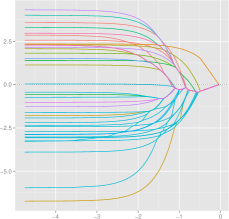
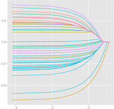
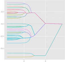
	tuning parameter $\lambda$ (log scale)
	$a)$ Cas-ANOVA	$b)$ Clusterpath	$c)$ Fused-ANOVA

Figure 1: Reconstructed phylogenetic trees for various weighting schemes. Families classified in the same order share the same color.

Multidimensional $\ell_{1}$ Clusterpath and fused-ANOVA.

In the previous example, we consider only one feature. In practice, one often has to consider multiple features at the same time. This is possible with our proposed weighted $\ell_{1}$-penalty. Indeed, as noted by Hocking et al. (2011), Problem (2) is separable on dimensions when considering the $\ell_{1}$-penalty, which is also the case for our weighted fused-ANOVA scheme. Thus, Clusterpath and fused-ANOVA algorithms solve the multidimensional problem in two steps:

1. First, they recover $p$ independent trees (one per dimension). This task can be easily executed in parallel.

2. Second they aggregate those $p$ trees in a consensus tree. This is done by considering the same penalty value ($\lambda$) corresponding to a given height in those trees. Two individuals $k$ and $\ell$ are in the same multidimensional cluster if they have been fused on every dimension.

This multidimensional classification is recovered on a grid of $\lambda$ in the clusterpath package and in the fusedanova package.

Note however that the classification recovered over all the dimensions is not necessarily better than those recovered on single, well-chosen features. We illustrate this point at the end in Section 8 on phylogenetic data: in a number of cases, the best agreement with the known phylogeny is obtained by a single-feature-based tree.

3 Optimality conditions and consequences

We start by characterizing Problem (2), giving elementary facts which are at the basis of most of our results. Note that the objective function in (2) is a nonsmooth function which is strictly convex in $\boldsymbol{\beta}$ and thus admits a unique solution when $\lambda\geq 0$. This solution can be characterized by the KKT (Karush-Kuhn-Tucker) conditions that may be derived thanks to subgradient calculus (see, e.g., Boyd and Vandenberghe, 2004). In the case at hand, $\boldsymbol{\beta}$ is optimal if, for all $k\in\left\{1,\dots,K\right\}$, $\boldsymbol{\beta}_{k}$ verifies the following subgradient equations:

$$\mathbf{0}_{p}=-n_{k}(\bar{\mathbf{y}}_{k}-\boldsymbol{\beta}_{k})+\lambda\sum_{\begin{subarray}{c}\ell:\ell\neq k\\ \boldsymbol{\beta}_{k}=\boldsymbol{\beta}_{\ell}\end{subarray}}w_{k\ell}\boldsymbol{\tau}_{k\ell}+\lambda\sum_{\begin{subarray}{c}\ell:\ell\neq k\\ \boldsymbol{\beta}_{k}\neq\boldsymbol{\beta}_{\ell}\end{subarray}}w_{k\ell}\frac{\partial\Omega(\boldsymbol{\beta}_{k}-\boldsymbol{\beta}_{\ell})}{\partial\boldsymbol{\beta}_{k}},$$ (3)

where $\bar{\mathbf{y}}_{k}=\sum_{i:\kappa(i)=k}\mathbf{y}_{i}/n_{k}$ is the vector of empirical means for the $k$th group across every feature. The $p$-dimensional vectors $\boldsymbol{\tau}_{k\ell}$ are such that, for any $k$, there exists $\ell\neq k$ with $\boldsymbol{\beta}_{k}=\boldsymbol{\beta}_{\ell}$ such that $\boldsymbol{\tau}_{k\ell}=-\boldsymbol{\tau}_{\ell k}$ and $\Omega(\boldsymbol{\tau}_{k\ell})\leq 1$. We omit the proof as it is a straightforward adaptation of the fused-Lasso subgradient equations (Hoefling, 2010) to the multidimensional case, with a general norm $\Omega$.

Interesting consequences arise when summing the subgradient equations (3) for all $\boldsymbol{\beta}_{k}$ which are “fused” in the same cluster, as stated in the following Lemma.

Lemma 1.

Consider a cluster $C=\left\{k:\boldsymbol{\beta}_{k}=\boldsymbol{\beta}_{C}\right\}$ formed by some $\boldsymbol{\beta}_{k}$, where $\boldsymbol{\beta}$ is the solution to (2). Then we have

$$\boldsymbol{\beta}_{C}=\bar{\mathbf{y}}_{C}-\frac{\lambda}{n_{C}}\sum_{\ell\notin C}w_{C\ell}\frac{\partial\Omega(\boldsymbol{\beta}_{C}-\boldsymbol{\beta}_{\ell})}{\partial\boldsymbol{\beta}_{C}},$$ (4)

where $n_{C}=\sum_{k\in C}n_{k},\bar{\mathbf{y}}_{C}=\sum_{k\in C}\bar{\mathbf{y}}_{k}/n_{C}$ and $w_{C\ell}=\sum_{k\in C}w_{k\ell}$.

Proof.

By summing (3) for all $k\in C$, we have

$$\mathbf{0}_{p}=-n_{C}\bar{\mathbf{y}}_{C}+n_{C}\boldsymbol{\beta}_{C}+\lambda\sum_{k,\ell\in C:k\neq\ell}w_{k\ell}\boldsymbol{\tau}_{k\ell}+\lambda\sum_{k\in C,\ell\notin C}w_{k\ell}\frac{\partial\Omega(\boldsymbol{\beta}_{k}-\boldsymbol{\beta}_{\ell})}{\partial\boldsymbol{\beta}_{k}}.$$

Then, by the KKT conditions, we must have $\boldsymbol{\tau}_{k\ell}=-\boldsymbol{\tau}_{\ell k}$ for some $k,\ell\in C$. Thus the third term on the left-hand side of the above expression vanishes by symmetry of the weights $w_{k\ell}$. Also notice that $\partial\Omega(\boldsymbol{\beta}_{k}-\boldsymbol{\beta}_{\ell})/\partial\boldsymbol{\beta}_{k}=\partial\Omega(\boldsymbol{\beta}_{k^{\prime}}-\boldsymbol{\beta}_{\ell})/\partial\boldsymbol{\beta}_{k^{\prime}}$ for any $k,k^{\prime}\in C,\ell\notin C$, and we easily get the desired result. ∎

4 Regularization path and tree structure

Characterization of the minimization Problem (2) in terms of its optimality conditions is essential in many ways. In particular, Lemma 1 allows us to characterize the regularization path of solutions $\left\{\boldsymbol{\beta}(\lambda),\lambda>0\right\}$ depending on the choices of $\Omega$ and $w_{k\ell}$. This is important for our problem since the shape of the path is actually the structure recovered between the conditions. This is also important since it may induce some computational properties that guarantee a low complexity of the associated fitting procedure. This section investigates which conditions must be imposed on the regularization path to ensure a structure that is fully satisfactory both in terms of algorithmic complexity and interpretability, namely, a balanced tree structure.

The mildest condition which is required is continuity of the regularization path, that is to say, of the function $\left\{\boldsymbol{\beta}(\lambda),\lambda>0\right\}$: without continuity, interpretability of the recovered structure is obviously out of reach. This property is straightforward for solutions of problems of form (2) which is strictly convex. However, continuity of the path is not enough to provide an interpretable structure, and we shall investigate conditions ensuring that the inferred structure is a tree. In terms of regularization path, it requires that any couple of parameters which have fused at a certain time $\lambda_{0}$ such that $\boldsymbol{\beta}_{k}(\lambda_{0})=\boldsymbol{\beta}_{\ell}(\lambda_{0})=\boldsymbol{\beta}_{C}$ cannot “split” anymore in the future, that is, for any value $\lambda>\lambda_{0}$ that would correspond to a higher level in the hierarchy of the tree. Insights on this remark can be found in Figure 2, where various regularization paths are plotted in the univariate case. Paths on the top and bottom left panels contain splits, while the remainders do not and lead to trees with different shapes the properties of which are discussed later in this section.

Piecewise quadratic path
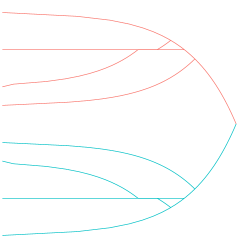
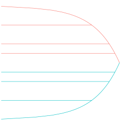
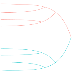
Piecewise linear path
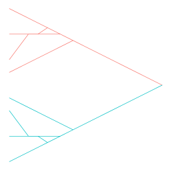
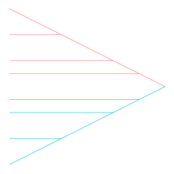
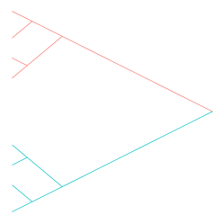
	not a tree (splits)	unbalanced tree	balanced tree

Figure 2: Various typologies of the regularization paths in the single feature case that lead to more or less interpretable structures.

Though highly desirable, guaranteeing a tree is complicated as the absence of splits in the path of (2) depends jointly on the choice of the weights $w_{k\ell}$ and on the fusing norm $\Omega(\cdot)$. In the following Theorem, we provide a simple generic choice for the weights that ensures the absence of splits in the general formulation with $\ell_{q}$-norms.

Theorem 1.

If $\Omega$ is an $\ell_{q}$-norm with $q\in\left\{1,\dots,\infty\right\}$ and $w_{kl}=n_{k}\cdot n_{\ell}$, the path of solutions $\left\{\boldsymbol{\beta}(\lambda):\lambda>0\right\}$ of (2) contains no splits.

The proof is postponed to Appendix A.1. Schematically, it investigates the subgradient equations of (2) and shows that given a solution at $\lambda_{0}$, we can always explicitly construct for $\lambda>\lambda_{0}$ a valid subgradient not involving any split. Theorem 1 generalizes the results of Hocking et al. (2011) obtained for $\Omega(\cdot)=\|\cdot\|_{1}$ in the clustering case when $w_{k\ell}=n_{k}=n_{\ell}=1$ to any $\ell_{q}$-norm $\Omega$.

A consequence of Theorem 1 is that the existing implementation of the $\ell_{2}$ Clusterpath – or any other $\ell_{q}$ solver – can be simplified by no longer considering the eventuality of splits with default weights (see Algorithm 1 in Hocking et al., 2011).

As said before, guaranteeing a tree-structure is the first step towards interpretability. As such, Theorem 1 characterizes an interesting family of problems. Still, the scope of arbitrary norms with uniform weights is not fully satisfactory because, even when the structure is a tree,

• the path is not a linear function of $\lambda$ in general, as illustrated on the first row of Figure 2. In this situation, detecting the events of fusion may be expensive. It might be impossible to provide an efficient algorithm to infer the structure at a low computational cost.

• the inferred structure may be highly unbalanced. By unbalanced, we mean a tree where two parameters initially close to one another at $\lambda=0$ fuse relatively late in the path of solutions. Such situations are depicted on the second column of Figure 2. It is obvious that disequilibrium may significantly narrow the potential for interpretability of the tree.

First, equilibrium of the inferred structure is a property that is mainly controlled by the $w_{k\ell}$. We cannot limit ourselves to $w_{k\ell}=n_{k}\cdot n_{\ell}$ and must exhibit weights sharing both the equilibrium and the non-split property. This will lead us to the distance-decreasing weights described in the next section.

Second, piecewise-linearity – and thus existence of a fast path-following algorithm – is a property of the norm $\Omega$. A solution path which is piecewise linear can be computed efficiently (and exactly) with a homotopy algorithm like the LARS for the LASSO (Efron et al., 2004). More generally, Rosset and Zhu (2007) give conditions for the existence of such a property in a broad penalized framework. These results are easily adapted to the case at hand, where we roughly have to differentiate Expression (4) over $\lambda$ to conclude: for $\Omega(\cdot)=\|\cdot\|_{q}$ any $q$-norm with $q\geq 1$, then

$$\frac{\partial\boldsymbol{\beta}_{C}}{\partial\lambda}=\frac{1}{n_{C}}\sum_{\ell\notin C}w_{C\ell}\ \mathrm{signs}(\boldsymbol{\beta}_{\ell}-\boldsymbol{\beta}_{C})\circ\frac{\left|\boldsymbol{\beta}_{\ell}-\boldsymbol{\beta}_{C}\right|^{q-1}}{\left\|\boldsymbol{\beta}_{\ell}-\boldsymbol{\beta}_{C}\right\|_{q}^{q-1}},$$ (5)

where $|\cdot|$ and $\mathrm{signs}(\cdot)$ apply element-wise and $\circ$ is the element-wise product. Application of Proposition 1 of Rosset and Zhu to these expressions implies that the path is piecewise linear only for $q\in\left\{1,\infty\right\}$. In other words, there must exist a homotopy algorithm to infer the structure between the conditions for the $\ell_{1}$ and $\ell_{\infty}$-norms. More generally, we could use any norm $\Omega$ that builds on $\ell_{1}$ and $\ell_{\infty}$ such as the OSCAR (Bondell and Reich, 2008a). Note, however, that there is no guarantee that the number of steps will be small in the homotopy algorithm for general weights. In fact, Mairal and Yu (2012) exhibits pathological cases for the LARS algorithm where the number of kinks in the piecewise linear path of solutions grows exponentially with the number of variables. Such cases can be transposed to the weighted fusion penalty with $\Omega(\cdot)=\|\cdot\|_{1}$, which corresponds to situations where there is a large number of splits along the path. To overcome this restriction and guarantee that the number of iterations required to fit the whole path of solutions will be small, we introduce in the next section a family of weights that ensures no split along the path of solutions for the particular case of the $\ell_{1}$-norm.

5 Distance-decreasing weights guaranteeing no split

In this section, we focus on the $\ell_{1}$-norm and generalize Theorem 1 to a larger class of weights that we call distance-decreasing weights, defined in Theorem 2. Indeed, although uniform weights ensure the absence of split, the recovered tree structure is often unbalanced. Intuitively, distance-decreasing weights should ensure that close neighbors fuse quickly. Here, we demonstrate that for such weights there is no split. Thus, the algorithm proposed by Hoefling (2010) for the generalized fused-Lasso is considerably simplified since there is no need to check for possible split events, and thus there is no need to solve potentially numerically unstable maximum flow problems.

Remark 1.

Note that the absence of splits does not ensure a fast algorithm. Indeed, the initialization of the generalized fused-Lasso algorithm is for most weights in $K^{2}$. We exhibit in Section 6 a subset of distance-decreasing weights for which initialization is linear and for which we can guarantee good statistical properties in Section 7.

Another advantage of the $\ell_{1}$-norm is that it brings separability across the $p$ features in (2), that is to say, that the $p$-dimensional problem splits into $p$ univariate problems. To recover a consensus classification, we first infer $p$ independent trees (one per dimension) and then aggregate those $p$ trees by considering the same penalty value $\lambda$. Thus, without loss of generality, we restrict the discussion to the following $\ell_{1}$ univariate problem which is a weighted generalized fused-Lasso problem:

$$\mathop{\mathrm{minimize}}_{\boldsymbol{\beta}\in\mathbb{R}^{K}}\frac{1}{2}\sum_{k=1}^{K}n_{k}\left(\bar{y}_{k}-\beta_{k}\right)^{2}+\lambda\ \sum_{k,\ell:k\neq\ell}w_{k\ell}|\beta_{k}-\beta_{\ell}|.$$ (6)

For this problem, we get the following result:

Theorem 2.

The path of solutions does not contain splits when weights are chosen such that

$$w_{k\ell}=n_{k}n_{\ell}\ f(\left|\bar{y}_{k}-\bar{y}_{\ell}\right|),$$

where $f(\cdot)$ is a decreasing positive function.

Schematically, the proof is based on two ingredients:

1. first, using geometrical arguments, it is possible to show that absence of splits is equivalent to preservation of the order along the path, that is to say, $\bar{y}_{k}\leq\bar{y}_{\ell}\Leftrightarrow\hat{\beta}_{k}(\lambda)\leq\hat{\beta}_{\ell}(\lambda)$;

2. second, by considering a problem that is dual to (6) as in Tibshirani and Taylor (2011) for the generalized Lasso, we show that distance-decreasing weights preserve the order.

The proof is detailed in Appendix A.2.

6 Fast homotopy algorithm for $\ell_{1}$ weighted penalties

In this section, we consider algorithmic issues when $\Omega$ is the $\ell_{1}$-norm. As in Section 5, we restrict the discussion to univariate Problem (6) and thus give the numerical complexity in the case $p=1$. For a $p$-dimensional problem, we aggregate the $p$ univariate trees by considering the same values of $\lambda$ for all trees.

An algorithm for general weights and its limitations.

Optimization problem (6) can be solved for general weights $w_{k\ell}$ by the homotopy algorithm proposed in Hoefling (2010) for the generalized fused-Lasso. This is also the solution retained in the clustering framework by Hocking et al. (2011). A schematic view of this algorithm adapted to (6) is depicted in 1.

Input: data, weights and initial groups $\left\{y_{i},w_{k\ell},\kappa\right\}$

Initialization for $\lambda=0$

Initialize $\beta_{k}$ parameters (equal to the empirical means $\bar{y}_{k}$)

Initialize the list of possible next events (only fusion at this stage)

while all groups are not fused do

       Find the next event (having the smallest $\lambda$), it can be a split or a fusion

       Update $\beta_{k}$ parameters accordingly

       Update the list of possible next events (fusion and split)

end while

Output: Directed acyclic graph (DAG) of fusion and split events and associated values of the parameters

Algorithm 1 Homotopy algorithm for the generalized fused-Lasso

This procedure for general weights has two major flaws that may have detrimental effects on its computational performance:

• By piecewise-linearity of the solution path, the total number of iterations (that is, the total number of events before all the groups have fused) is bounded. However, by rewriting (6) as a Lasso problem – which only requires straightforward algebra – we may construct pathological cases where there are $(3^{K}+1)/2$ linear segments in the path of solutions (see Mairal and Yu, 2012), a complexity that we cannot afford even for a moderate number of conditions $K$.

• While detecting fusion events in Algorithm 1 may be cheap since it roughly only requires calculation of the slopes $\partial\beta_{k}(\lambda)/\partial\lambda$, checking for the possibility of split events boils down to maximum-flow problems the resolution of which at large scale may clearly be a bottleneck (see Hoefling, 2010).

To circumvent these limitations, we shall consider weights that prevent split events. Although the choice $w_{k\ell}=n_{k}n_{\ell}$ has been shown to prevent splits in Theorem 1, it will typically lead to fusion events occurring very late (that is, for large $\lambda$), even between groups having close empirical means. This corresponds to an unbalanced tree structure between the conditions, which is hardly interpretable. On the contrary, using the family of distance-decreasing weights, introduced in Section 5, prevents split events and leads to a balanced tree structure. In this case the total number of events is exactly $K-1$, which is the number of iterations required to fuse $K$ groups into 1, assuming that there cannot be a fusion of more than two groups at once. As for the maximum-flow problems, they are completely eluded from the algorithm with these weights. Still, we have to take into account the cost of detecting successive fusion events and of updating the coefficients $\beta_{k}(\lambda)$ along the $K-1$ steps. In the next paragraph, we propose a solution inducing a global complexity of $\mathcal{O}(K\log(K))$ for a given choice of weights belonging to the family of distance-decreasing weights.

Weights with an $\mathcal{O}(K\log(K))$ implementation.

First we need to define the next time a fusion event is going to happen. We proceed mainly as in Hoefling (2010) for the one-dimensional fused-Lasso signal approximator, except that the initial ordering is not defined by the neighborhood between the coefficients, but by the ordering of the empirical means $\bar{y}_{k}$. And thanks to the property of the distance-decreasing weights, this ordering remains the same throughout the algorithm, which allows us to compute the path in $\mathcal{O}(K\log K)$ operations. Here are some details.

At the initialization step, one has $\lambda_{0}=0$, and the next time a fusion occurs is

$$t(\lambda)=\mathop{\mathrm{arg\ min}}_{t_{k\ell}(\lambda)>\lambda_{0}}t_{k\ell},\quad t_{k\ell}(\lambda)=\lambda_{0}-(\beta_{k}(\lambda_{0})-\beta_{\ell}(\lambda_{0}))\left(\frac{\partial\beta_{k}}{\partial\lambda}(\lambda_{0})-\frac{\partial\beta_{\ell}}{\partial\lambda}(\lambda_{0})\right)^{-1}.$$ (7)

In words, it is the smallest value of $\lambda$ among all the values such that two coefficients fuse. The main cost in (7) is due to the calculation of the slopes $\partial\beta_{k}/\partial\lambda$ at $\lambda_{0}=0$. Note that $\beta_{k}(0)=\bar{y}_{k}$, and by Lemma 1 and (5), one has

$$\frac{\partial\beta_{k}}{\partial\lambda}(0)=-\frac{1}{n_{k}}\sum_{\ell\neq k}w_{k\ell}\ \mathrm{signs}(\bar{y}_{k}-\bar{y}_{\ell}).$$ (8)

For general weights $w_{k\ell}$, computing these slopes for all $k$ requires $\mathcal{O}(K^{2})$ operations and is the limiting factor of the algorithm. However, we provide a $\mathcal{O}(K\log(K))$ procedure for a special case of our distance-decreasing weights that we call “exponentially adaptive weights” because of their statistical properties (see Section 7). They are defined by

$$w_{k\ell}=n_{k}n_{\ell}\exp\{-\alpha\sqrt{n}|\bar{y}_{k}-\bar{y}_{\ell}|\},\quad\alpha>0,$$ (9)

for $\alpha$ a positive constant. The key idea to achieve $\mathcal{O}(K\log(K))$ complexity with these weights is that each slope can be computed as the sum of two terms, for which there exists a simple recurrence formula: first, we order the $\bar{y}_{k}$ in decreasing order, which can be done in $\mathcal{O}(K\log(K))$ operations. Assuming this is done, we obtain

$$\frac{\partial\beta_{k}}{\partial\lambda}(0) =-\sum_{\ell\neq k}n_{\ell}\ \mathrm{signs}(\bar{y}_{k}-\bar{y}_{\ell})\ \exp\left\{-\alpha\sqrt{n}|\bar{y}_{k}-\bar{y}_{\ell}|\right\}$$

$$=\sum_{\ell<k}n_{\ell}\exp\left\{-\alpha\sqrt{n}(\bar{y}_{\ell}-\bar{y}_{k})\right\}-\sum_{\ell>k}n_{\ell}\exp\left\{-\alpha\sqrt{n}(\bar{y}_{k}-\bar{y}_{\ell})\right\}$$

$$=\exp\left\{\alpha\sqrt{n}\bar{y}_{k}\right\}\underbrace{\sum_{\ell<k}n_{\ell}\ \exp\left\{-\alpha\sqrt{n}\bar{y}_{\ell}\right\}}_{L_{k}}-\exp\left\{-\alpha\sqrt{n}\bar{y}_{k}\right\}\underbrace{\sum_{\ell>k}n_{\ell}\ \exp\left\{\alpha\sqrt{n}\bar{y}_{\ell}\right\}}_{R_{k}}.$$

The recurrence formulae are $R_{k+1}=R_{k}+n_{k}\exp\left\{-\alpha\bar{y}_{k}\right\}$ and $L_{k-1}=L_{k}+n_{k}\exp\left\{\alpha\bar{y}_{k}\right\}$. By this means, the initial slopes (8) and thus the first fusion time can be computed in $\mathcal{O}(K\log(K))$.

Then, for each of the $K-1$ steps of the algorithm, we only need to update the two slopes and the two coefficients which are currently fusing. This only requires a constant number of operations. Concerning the next fusion time, however, the new minimum among the updated $t_{k\ell}(\lambda_{0}^{+})$ is found in $\log(K)$ if stored in an appropriate structure. This way we can reach $\mathcal{O}(K\log(K))$ for the global complexity.

As a final remark, note that we use the same storage solution – namely a binary tree – as did Hoefling (2010) for the one-dimensional fused-Lasso. By this means, we maintain the memory requirement at a low level that only grows linearly in $K$.

An embedded cross-validation procedure.

Providing the whole path of solutions is clearly interesting for interpretability, since we force it to be a tree by means of an appropriate weighting scheme coupled with the $\ell_{1}$-norm for fusion. Still, it is always necessary to provide a practical way to choose the tuning parameter, which corresponds in the case at hand to choosing the level at which to cut the tree. This also gives a fixed classification between the initial conditions.

When the number $K$ of prior groups is smaller than $n$ (e.g., in the ANOVA settings), a natural cross-validation (CV) error can be defined. Although CV is often incriminated for being time-consuming, it is possible in this case to rely on the tree structure of the solution – or DAG in the case where split is allowed in the algorithm – to enhance the performance. Indeed, we can first build a tree using a training set (in which all prior groups are present) and then assess its performance by measuring its ability to predict the remaining individuals of the test set for any given value of $\lambda$. Here, we perform the CV on a predefined grid of $L$ values of $\lambda$ because the fusion times will be different for every new training set and it would be memory intensive to store the CV-error for every of those fusion time.

To be more specific, we consider a split of the data in a train set $\mathcal{D}$ and a test set $\mathcal{T}$ such that each prior group is represented in the train set. Using $\mathcal{D}$, we recover a fused-ANOVA tree and an estimator $\,\hat{\!\boldsymbol{\beta}}^{\raisebox{-3.01389pt}{\scriptsize$\mathcal{D}$}}_{\kappa(i)}(\lambda)$. The test error on $\mathcal{T}$ is

$$\mathrm{CV}_{\mathrm{err}}(\mathcal{D},\mathcal{T},\lambda)=\sum_{i\in{\mathcal{T}}}\left(y_{i}-\,\hat{\!\boldsymbol{\beta}}^{\raisebox{-3.01389pt}{\scriptsize$\mathcal{D}$}}_{\kappa(i)}(\lambda)\right)^{2}.$$ (10)

A naive approach to computing (10) is to consider each prior group at a time on a grid of $\lambda$. Computing the prediction based on a given fitted regularization path requires $\mathcal{O}(\log(K))$ operations to search through the tree of solutions. This has to be done for the $K$ prior groups and for the $L$ values in the grid of $\lambda$. Hence, computing the sum (10) naively has a total complexity of $\mathcal{O}(LK\log(K))$ (which dominates the complexity in $\mathcal{O}(K\log(K))$ of the fit itself!).

On the contrary, our embedded cross-validation procedure takes advantage of the tree structure of the fit in the computations whenever possible. Indeed, along the branch of a cluster $C$, the estimator $\,\hat{\!\boldsymbol{\beta}}^{\raisebox{-3.01389pt}{\scriptsize$\mathcal{D}$}}_{\kappa(i)}(\lambda)$ is a piecewise linear function of $\lambda$ and thus the error (10) is a piecewise quadratic function of $\lambda$. The coefficients of this quadratic function are easily updated when constructing the tree, and the error along this branch is computed in $\mathcal{O}(1)$ for any $\lambda$ rather than $\mathcal{O}(|C|\log(K))$. More precisely the error in (10) of cluster $C$ decomposes thanks to the Huygens formula as

$$\sum_{i\in\mathcal{T}:\kappa(i)\in C}\left(y_{i}-\,\hat{\!\boldsymbol{\beta}}^{\raisebox{-3.01389pt}{\scriptsize$\mathcal{D}$}}_{\kappa(i)}(\lambda)\right)^{2}=\sum_{i\in\mathcal{T}:\kappa(i)\in C}(y_{i}-\bar{\mathbf{y}}_{C}^{\mathcal{T}})^{2}+n_{C}^{\mathcal{T}}\left(\bar{\mathbf{y}}_{C}^{\mathcal{T}}-\,\hat{\!\boldsymbol{\beta}}^{\raisebox{-3.01389pt}{\scriptsize$\mathcal{D}$}}_{\kappa(i)}(\lambda)\right)^{2},$$

where $n_{C}^{\mathcal{T}}=\mathrm{card}(\left\{i\in\mathcal{T}:\kappa(i)\in C\right\})$ and $\bar{\mathbf{y}}_{C}^{\mathcal{T}}$ is the empirical mean of individuals of cluster $C$, i.e.,

$$\bar{\mathbf{y}}_{C}^{\mathcal{T}}=\frac{1}{n_{C}^{\mathcal{T}}}\sum_{i\in\mathcal{T}:\kappa(i)\in C}y_{i}.$$

It is difficult to assess exactly the gain brought by using the tree structure for computing the CV error in general. Indeed, it depends on the tree itself, the length of its branches, its height and so on. Assuming a binary balanced tree of height $\log(K)$, with branches of equal length and an equally spaced grid of $\lambda$, we can show that the complexity is in $\mathcal{O}(LK/\log(K))$. If some groups fused rapidly (as with the fused-ANOVA weights), the gain could be even greater. In practice (see Figure 3.c), we often see a ten-fold difference between our CV procedure and a naive implementation.

Timings.

We implemented both the general and the without-split version of Algorithm 1 in C++ embedded in an R-package called fusedanova distributed on R-forge. It contains a wide family of weights which are not mentioned in this paper due to space requirements. Figure 3 illustrates the rather good performance of our algorithm and implementation through three numerical experiments:

1. In the left panel, we illustrate the capability of our method to treat large scale problems extremely fast: we generate a size-$n$ vector $\mathbf{y}$ such that $y_{i}\sim\mathcal{N}(0,1)$ and assume $n=K$, meaning one condition per group. We vary $n$ from $10^{2}$ to $10^{8}$ and record the corresponding timing in seconds. We apply our method with the exponentially adaptive weights and average over 10 trials. As can be seen, we can reconstruct a tree on $n=10^{6}$ observations in about 10 seconds.

2. The middle panel illustrates the gain in runtime due to the fact that we no longer have to check for splits in the homotopy algorithm using a maximum-flow solver. We generate data as in the preceding experiment but with $K$ conditions each containing $n_{k}=20$ replicates. When $K=10^{3}$, the gain in seconds brought by not checking for the possibility of splits is of almost 2 orders of magnitude.

3. The right panel illustrates the performance of our embedded CV procedure compared to the naive implementation. We used the same settings as in the previous experiment.

timings in seconds (log)
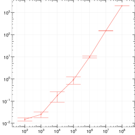
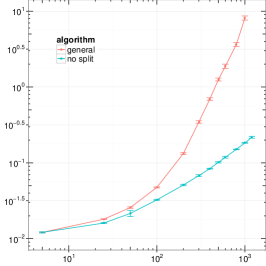
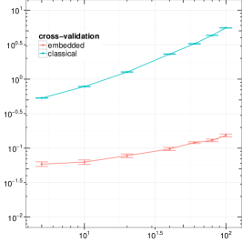
	number of conditions $K$ (log)

Figure 3: timing experiments: $a)$ time in seconds as a function of the number of conditions $K$; $b)$ timing comparison for general/without-split algorithm; and $c)$ timing comparison for naive/embedded cross-validation.

We tried other implementations to solve (6) such as the Clusterpath package by Hocking et al. (2011), the flsa package by Hoefling (2010) or the genlasso package by Tibshirani and Taylor (2011). These implementations do not fully exploit the structure of the problem and have runtimes considerably longer than ours, even for moderate $K$. Thus, we do not report their timings here.

7 Statistical guarantees

Asymptotic settings.

To discuss the asymptotic properties of our exponentially adaptive weights (9), we shall consider the following univariate ANOVA model

$$y_{i}=\beta_{\kappa(i)}^{\star}+\varepsilon_{i},\quad\text{s.t.}\quad\mathbb{E}(\varepsilon_{i})=0,\ \mathrm{Var}(\varepsilon_{i})=\sigma^{2},\quad i=1,\dots,n,$$ (11)

where $\boldsymbol{\beta}^{\star}=(\beta_{1}^{\star},\dots,\beta_{K}^{\star})$ is the true vector of parameters and $\varepsilon_{i}$ are iid residuals. The correct structure between the coefficients – or classification – in $\boldsymbol{\beta}^{\star}$ is denoted by $\mathcal{A}^{\star}=\left\{(k,l):\beta_{k}^{\star}=\beta_{\ell}^{\star}\right\}$. A usual technical assumption is to consider designs the associated gram matrices of which converge to positive definite matrices. In the one-way ANOVA settings, we just need to assume that when $n\to\infty$, then $n_{k}/n\to\rho_{k}<\infty$ for all $k=1,\dots,K$. We denote by $\mathbf{D}$ the corresponding asymptotic covariance matrix which is a $K$-diagonal matrix with diagonal entries equal to $\rho_{1},\dots,\rho_{K}$.

In the univariate case like in (11), the estimator associated with Problem (2) using the $\ell_{1}$-norm for fusion is

$$\,\hat{\!\boldsymbol{\beta}}^{(n)}=\mathop{\mathrm{arg\ min}}_{\boldsymbol{\beta}\in\mathbb{R}^{K}}\frac{1}{2}\sum_{k=1}^{K}n_{k}\left(\bar{y}_{k}-\beta_{k}\right)^{2}+\lambda_{n}\ \sum_{k\neq\ell}w_{k\ell}|\beta_{k}-\beta_{\ell}|,$$ (12)

which is just a rewriting of (6) where the dependency on $n$ of the estimator and the tuning parameter is stated explicitly for the purpose of asymptotic analysis. Similarly, we denote by $\hat{\mathcal{A}}_{n}=\left\{(k,\ell):\hat{\beta}_{k}^{(n)}=\hat{\beta}_{\ell}^{(n)}\right\}$ the estimated group structure.

Exponentially adaptive weights and the fused-ANOVA.

In this paragraph, we study the exponentially adaptive weights, which we recall here:

$$w_{k\ell}^{\text{FA}}=n_{k}n_{\ell}\exp\{-\alpha\sqrt{n}|\bar{y}_{k}-\bar{y}_{\ell}|^{\gamma}\},\quad\alpha,\gamma>0.$$

We show that they enjoy some “oracle properties” in the sense of Fan and Li (2001), that is, both $i)$ right model identification (recovering the true classification $\mathcal{A}^{\star}$) and $ii)$ optimal estimation rate $\sqrt{n}$. In the context of the penalized ANOVA problem (12), we denote these weights by $w_{k\ell}^{\text{FA}}$ and call the associated estimator the fused-ANOVA. These weights are adaptive as in the adaptive-Lasso of Zou (2006): it is known that raw $\ell_{1}$ methods like the Lasso do not enjoy the aforementioned oracle properties, yet this can be fixed by choosing judicious weights that depend on an estimator of $\boldsymbol{\beta}^{\star}$ which is asymptotically $\sqrt{n}$-consistent – like the ordinary least squares, which equals $(\bar{y}_{1},\dots,\bar{y}_{K})$ in the case at hand. Here we are interested in the differences between the entries of $\,\hat{\!\boldsymbol{\beta}}$; thus the quantity $\sqrt{n}|\bar{y}_{k}-\bar{y}_{\ell}|$ seems quite natural in (9).

While studying the asymptotic of our estimator, we came across the proposal of Bondell and Reich (2008b) for adaptive weights: they consider Problem (12) with additional constraints on the $\beta_{k}$’s – that must sum to zero – and the following weights, which we refer to as the Cas-ANOVA weights:

$$w_{k\ell}^{\text{CA}}=\frac{\sqrt{n_{k}+n_{\ell}}}{|\bar{y}_{k}-\bar{y}_{\ell}|}.$$ (13)

As we shall see, though quite interesting, Cas-ANOVA weights are adaptive on a smaller range of $\lambda_{n}$ than are fused-ANOVA weights. Moreover, they lead to splits. Thus, we believe that fused-ANOVA is computationally and statistically more efficient for solving Problem (12).

We now proceed to the Theorem stating the required conditions on $\lambda_{n}$ for the fused-ANOVA to enjoy the oracle properties.

Theorem 3 (Oracle properties).

Suppose that $\lambda_{n}n^{3/2}\exp\left\{-\alpha\sqrt{n}\right\}\to 0$ and $\lambda_{n}n^{3/2}\to\infty$ when $n\to\infty$. Then the fused-ANOVA enjoys asymptotic normality and consistency for recovering the true classification, i.e.,

$$\sqrt{n}\left(\hat{\boldsymbol{\beta}}^{(n)}-\boldsymbol{\beta}^{\star}\right)\ \to_{d}\mathcal{N}(\mathbf{0},\sigma^{2}\mathbf{D}^{-1})\quad\text{and}\quad\mathbb{P}(\hat{\mathcal{A}}_{n}=\mathcal{A}^{\star})\to 1\text{ when }n\to\infty.$$

The proof is postponed to Appendix A.3 and roughly follows that of Zou. We have, however, some comments related to this Theorem.

Remark 2 (On the exponentially adaptive weights).

The key idea behind this theorem is that when $n$ goes to infinity, then $w_{k\ell}^{\text{FA}}/\sqrt{n}$ goes to infinity if $(k,\ell)\in\mathcal{A}^{\star}$ and to zero exponentially fast if $(k,\ell)\notin\mathcal{A}^{\star}$. This is due to the joint effect of the $\sqrt{n}$-consistency of the $\bar{y}_{k}$ and of the exponential. This is to be compared with Cas-ANOVA weights, where, when $n\to\infty$, $w_{k\ell}^{\text{CA}}/\sqrt{n}$ goes to infinity if $(k,\ell)\in\mathcal{A}^{\star}$, but only to a constant if $(k,\ell)\notin\mathcal{A}^{\star}$.

Remark 3 (On the range of $\lambda_{n}$).

Theorem 3 is true for a large range of $\lambda_{n}$ values. In particular it is true for a constant $\lambda_{n}$. Asymptotically all groups belonging to the same class fuse almost immediately (i.e., for small values of $\lambda$ of the order $n^{3/2}\exp\left\{-\alpha\sqrt{n}\right\}$) and the groups belonging to different classes fuse for very large $\lambda$, i.e., of the order $n^{3/2}$.

Numerical illustration in the univariate case.

We generate data from model (11) as follows, for $K$ the number of prior groups and $n$ being fixed: the true vector of parameters $\boldsymbol{\beta}^{\star}$ is composed of $K$ entries picked up randomly among $\left\{1,2,3\right\}$, such that the correct structure $\mathcal{A}^{\star}$ is always composed of 3 groups. Then, the initial group sizes $n_{k}$ are drawn from a multinomial distribution $\mathcal{M}(n,(p_{1},\dots,p_{K}))$ with $p_{k}=1/K$ for all $k=1,\dots,K$, such that the $n_{k}$ are approximately balanced. Finally, we let $\varepsilon_{i}\sim\mathcal{N}(0,1)$ to generate the vector of data $\mathbf{y}=(y_{1},\dots,y_{n})$.

We compare the capability of three weighting schemes to recover the true grouping $\mathcal{A}^{\star}$, namely the fused-ANOVA weights, the Cas-ANOVA weights, and the so-called default weights corresponding to $w_{k\ell}=n_{k}n_{\ell}$, which are not adaptive but produce a path of solutions that contains no split. Such weights correspond to the Clusterpath weights adapted to the ANOVA setup. We use our own code for each method. Typically, the computational burden required by Cas-ANOVA is huge, compared to the other two procedures as the path of solutions may contain splits. Qualitatively, the difference would be as in Figure 3, middle panel. Thus, we typically force the algorithm not to split when using the Cas-ANOVA weights.

We generate data as specified below, and for each procedure we check whether there exists at least one $\lambda$ for which the correct structure is identified along the path of solutions. The probability of true support recovery is evaluated by replicating this experiment a large number of times ($8096$ times). To investigate the asymptotic behavior of each method, we vary $n$ from 50 to 1,000 and consider two scenarios for the initial number of groups $K$. First, $K$ is fixed at $10$ such that the number of elements in each group grows with $n$. In the second scenario, $K$ grows with $n$ through the relationship $K=2.5\cdot\log(n)$. The results are reported on Figure 4, with the first (resp. the second) scenario on the left (resp. the right) panel. The results confirm Theorem 3. The two adaptive procedures, Cas-ANOVA, and to a greater extent, fused-ANOVA, dominate the non-adaptive weights. As expected from Section 7, fused-ANOVA always dominate Cas-ANOVA, as experienced in other scenarios (e.g., $K=C\cdot\sqrt{n}$) not reported here to save space.

	$a)\ K=\text{cst.}$	$b)\ K=C\log(n)$
$\hat{\mathbb{P}}(\hat{\mathcal{A}}_{n}=\mathcal{A}^{\star})$
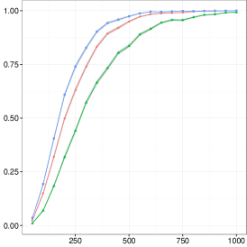
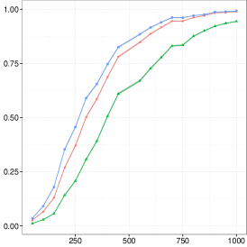
	sample size $n$

Figure 4: Univariate case: estimated probability of consistency as a function of the sample size $n$, for various weights and in two scenarios: the number of initial groups $K$ is either $a)$ fixed to a constant (10) or $b)$ increases in $C\log(n)$ with $C=2.5$. The true number of groups in $\mathcal{A}^{\star}$ is 3.

Numerical illustration in the bivariate case.

Theorem 3 characterizes the asymptotic of the fused-ANOVA estimators when considering one dimension at a time. Concerning the multidimensional setting, there are two situations. On the first hand, there exists a dimension such that all the true groups are different, i.e $\beta_{kj}^{\star}\neq\beta_{\ell j}^{\star}$. In this case, our theorem guarantees that, using this particular dimension, the recovered classification will converge to the true one. On the second hand, there exists no dimension such that the true groups are all different. In that case, we have no theoretical guarantee to support the fused-ANOVA weights. It is nonetheless possible to aggregate the classification obtained in each dimension to a consensus classification. For a given $\lambda$, two individuals $k$ and $\ell$ are in the same multidimensional cluster if they have been fused on every dimension.

In order to evaluate empirically the performance of the aggregation step, we consider a two dimensional classification problem with three classes and two scenarii. Each prior group is drawn from one of three classes. In the first scenario, the three classes have different means on the first dimension and the same mean on the second dimension. The mean vectors are $(1,1.5);(2,1.5);(3,1.5)$, as in top left panel of Figure 5. In the second scenario, both dimensions are informative: the first dimension separates classes $\left\{1,2\right\}$ from $\left\{3\right\}$ while the second dimension separates classes $\left\{1,3\right\}$ from $\left\{2\right\}$. The mean vectors are $(1,1);(1,2);(2,1)$, as in top right panel of Figure 5). We increase the difficulty in each scenario by adding a Gaussian noise with increasing standard deviation $\sigma$. Results in Figure 5 corresponds to the estimated probability of true classification recovery along the path, averaged over 2,000 runs.

$\bar{\mathbf{y}}_{k,1}$
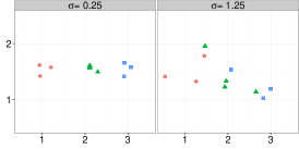
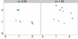
	$\bar{\mathbf{y}}_{k,2}$	$\bar{\mathbf{y}}_{k,2}$
$\hat{\mathbb{P}}(\hat{\mathcal{A}}_{n}=\mathcal{A}^{\star})$
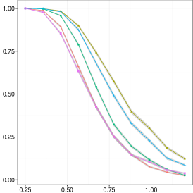
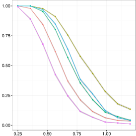
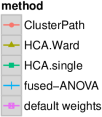
	standard deviation $\sigma$

Figure 5: Bivariate example: estimated probability of consistency as a function of the noise standard deviation $\sigma$, for various clustering methods. The initial number of groups $K$ fixed to a constant (10). The true number of groups in $\mathcal{A}^{\star}$ is 3.

In both scenarii, the fused-ANOVA weights with aggregation outperform the multidimensional $\ell_{2}$-Clusterpath as well as the single linkage hierarchical clustering. The Ward hierarchical clustering shows better performance but at a much higher computational cost.

In this simple multidimensional numerical study, we always aggregate the classification over the dimensions. However, this aggregation is not necessarily better than performing classification on single, well-chosen feature. We illustrate this point in the following section on phylogenetic data.

8 A complete example in phylogeny

Evolutionary trees – sometimes referred to as “trees of life” – are one of the most emblematic hierarchical representations in computational biology. They are typically used in phylogenetics to compare biological species based on their similarities regarding one or several features. These features could be phenotypic traits or genetic characteristics. In these tree structures, each node corresponds to a taxonomic unit, the root node being the most recent common ancestor to all leaves on the tree. All other intermediate nodes between root and leaves represent the taxonomic knowledge between the species of interest. The study depicted in Vetrovsky and Baldrian (2013) enters this framework by more specifically considering features associated with bacterial genomes to determine the phylogenetic relationships between the taxa. The data set consists of various genetic features associated with $n=1,690$ complete bacterial genomes classified in $K=903$ known bacterial species.

We apply our method on this data set to assess its capability of capturing the true underlying taxonomic structure. To do so, we consider the following genetic features to construct the hierarchy: the number of known genes, the number of known proteins and the genome size (measured by the number of bases in millions). We apply the univariate model (6) on each feature to reconstruct a tree structure. The indexing function $\kappa$ is built from the lowest level of classification available that splits the genomes into $K=903$ bacterial species. We use the default weights and the fused-ANOVA weights (9) with $\alpha$ chosen specifically for each feature (see below). We also apply hierarchical clustering using Ward’s criterion and starting from the known classification in bacterial species. Hierarchical clustering is applied individually on each feature, as well as across the three features using the Euclidean distance to build the similarity matrix. To assess the relevance of the inferred trees, we compare them with various levels of the known taxonomic classification above the species level, namely genus (470 groups), family (216 groups), order (100 groups), class (46 groups) and phylum (27 groups). To this end, we compute the best adjusted rand-index between the respective reference classifications and the classifications obtained by cutting an inferred tree at all the possible levels of the hierarchy. As an example, we report in Figure 6 a subset of the tree inferred by the fusion penalty with fused-ANOVA weights and the cutting level that leads to the best performance in terms of adequacy with the true phylum taxonomy.

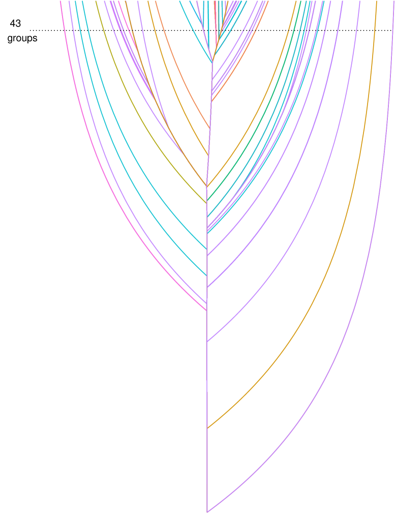
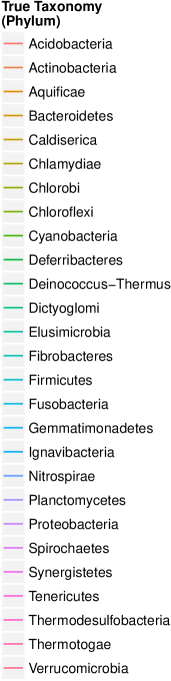
Figure 6: Tree reconstructed with fused-ANOVA from the “Size.Mb” trait (Adjusted Rand-Index=0.71). Projected colors correspond to the true taxonomy (phylum).

More quantitative results are reported in Figure 7, with the adjusted rand indexes for the taxonomic classifications in terms of phylum, order and family, using either the number of genes, the number of proteins or the genome size as the feature variable for classification. We also represent the consensus/multidimensional classifications either obtained by aggregating the three univariate fused-ANOVA trees or by considering the three features together for Ward hierarchical clustering. Note that for the fused-ANOVA weights, we apply our method on a grid of $\alpha$ and report the results obtained for the best $\alpha$ in terms of adjusted rand-index.

Adjusted Rand-Index
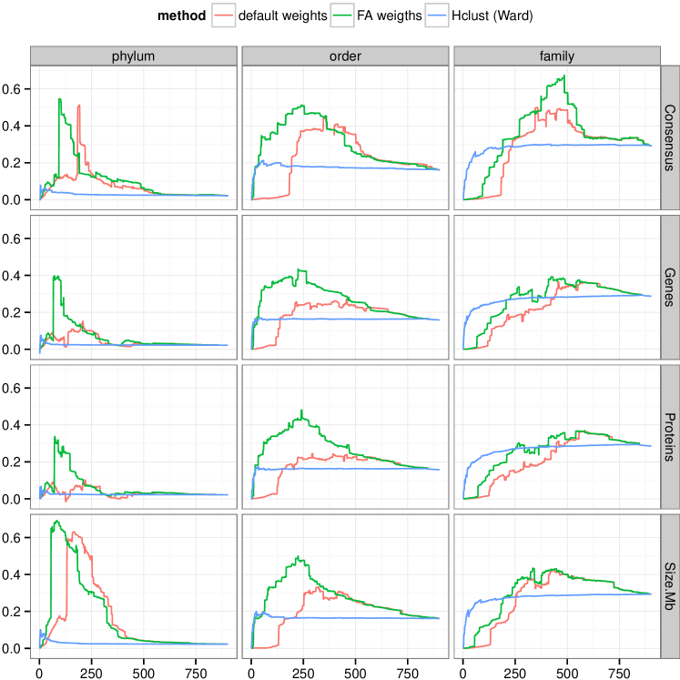
	number of groups

Figure 7: Adequacy of various tree-based clustering methods to different levels of phylogenetic classification.

First, we notice that the fused-ANOVA weights always outperform the default weights. This is expected since the former weights are a special case of the latter when $\alpha\to 0$. Second, we note that the consensus classification – or the one obtained by multivariate hierarchical clustering – is not always the best choice. This is particularly obvious for the phylum classification, where the “size” feature leads to very good results in terms of adjusted rand-index. These results considerably deteriorate for the consensus classification, due to the relatively poor results obtained from the “genes” and “proteins” features. Finally, the most striking result in Figure 7 is that the fusion penalty approaches clearly outperform the Ward hierarchical clustering. At first glance, one might argue that the weighting scheme used in fused-ANOVA is responsible for such good performance. However, the fusion penalty with default weights remains competitive in a few cases. This supports the fact that the regularizing virtue of the fusion penalty is of great help when the problem size is high.

Appendix A Proofs

A.1 Theorem 1 (absence of splits with norms)

For the sake of brevity the proof is detailed only in the clustering framework, i.e., when $\kappa(i)=i$ and $n_{k}=1$ for all $k=1,\dots,K$. The generalization to groups with more than one individual is straightforward and follows the exact same line.

Consider the objective function in (2) and a time $\lambda_{0}$ at which we have a valid set of clusters. It is obvious that clusters containing only one individual cannot split. We will thus consider clusters grouping together more than one element. We denote by $C=\left\{k:\beta_{k}(\lambda_{0})=\beta_{C}(\lambda_{0})\right\}$ such a cluster, with $\beta_{C}$ the current estimated mean. For unitary weights, Lemma 1 implies that

$$\mathbf{0}_{p}=-\bar{\mathbf{y}}_{C}+\boldsymbol{\beta}_{C}+\lambda_{0}\sum_{i\notin C}\frac{\partial\Omega(\boldsymbol{\beta}_{C}-\boldsymbol{\beta}_{i})}{\partial\boldsymbol{\beta}_{C}}(\lambda_{0}).$$

Subtracting the above equation from the subgradient equation (3) for $i\in C$, one has

$$\bar{\mathbf{y}}_{C}-\mathbf{y}_{i}+\lambda_{0}\sum_{j\in C}\boldsymbol{\tau}_{ij}(\lambda_{0})=\mathbf{0}_{p}.$$ (14)

We now consider any time $\lambda\geq\lambda_{0}$ such that no fusion has occurred. Let us show that for $\boldsymbol{\tau}_{ij}(\lambda)=\frac{\lambda_{0}}{\lambda}\boldsymbol{\tau}_{ij}(\lambda_{0})$, it is possible to solve the KKT conditions, and thus show that no split occurs.

First, the proposed $\boldsymbol{\tau}_{ij}(\lambda)$ are valid subgradients as $\Omega(\boldsymbol{\tau}_{ij}(\lambda))\leq 1$ since $\Omega(\boldsymbol{\tau}_{ij}(\lambda_{0}))\leq 1$ and $\lambda>\lambda_{0}$. Second, for this particular choice of subgradient and thanks to (14), the KKT conditions for all $C$ and all $i\in C$ simplify as follows:

$$\boldsymbol{\beta}_{C}-\mathbf{y}_{i}+\lambda\sum_{j\in C}\frac{\lambda_{0}}{\lambda}\boldsymbol{\tau}_{ij}(\lambda_{0})+\lambda\sum_{C^{\prime}\neq C}|C^{\prime}|\frac{\partial\Omega(\boldsymbol{\beta}_{C}-\boldsymbol{\beta}_{C^{\prime}})}{\partial\boldsymbol{\beta}_{C}}(\lambda)\\ =\boldsymbol{\beta}_{C}-\bar{\mathbf{y}}_{C}+\lambda\sum_{C^{\prime}\neq C}|C^{\prime}|\frac{\partial\Omega(\boldsymbol{\beta}_{C}-\boldsymbol{\beta}_{C^{\prime}})}{\partial\boldsymbol{\beta}_{C}}(\lambda).$$

It now remains to check that we can find a $\boldsymbol{\beta}$ which zeroes this subgradient equation. Note that for all $C^{\prime}\neq C$, the differential $\partial\Omega(\boldsymbol{\beta}_{C}-\boldsymbol{\beta}_{C^{\prime}})/\partial\boldsymbol{\beta}_{C}(\lambda)$ is well defined. Then, by multiplying the above expression by $|C|$, we obtain the gradient of the following objective function

$$\frac{1}{2}\sum_{i=1}^{n}\left\|\mathbf{y}_{i}-\boldsymbol{\beta}_{i}\right\|_{2}^{2}+\lambda\sum_{C,C^{\prime}:C\neq C^{\prime}}|C|\cdot|C^{\prime}|\ \Omega(\boldsymbol{\beta}_{C}-\boldsymbol{\beta}_{C^{\prime}}).$$

This is a strictly convex problem admitting one unique solution which is solved by zeroing its gradient. Thus we necessarily have

$$\boldsymbol{\beta}_{C}-\bar{\mathbf{y}}_{C}+\lambda\sum_{C^{\prime}\neq C}|C^{\prime}|\frac{\partial\Omega(\boldsymbol{\beta}_{C}-\boldsymbol{\beta}_{C^{\prime}})}{\partial\boldsymbol{\beta}_{C}}(\lambda)=\mathbf{0}_{p},$$

which ends the proof.

A.2 Theorem 2: absence of splits with distance-decreasing weights in 1-d

For the sake of brevity the proof is detailed only in the case where $\kappa(i)=i$ and $n_{k}=1$ for all $k=1,\dots,K$. The generalization to groups with more than one individual is straightforward, seeing that we can replace a group $\kappa(i)$ by $n_{\kappa(i)}$ individuals with value $\sum_{j}y_{j}/n_{\kappa(i)}$. Also, when $\Omega\equiv\ell_{1}$, the proof remains valid but should be done separately on each dimension.

Throughout the proof, we may thus consider the estimator defined by

$$\,\hat{\!\boldsymbol{\beta}}(\lambda)=\mathop{\mathrm{arg\ min}}_{\boldsymbol{\beta}\in\mathbb{R}^{n}}\frac{1}{2}\sum_{i=1}^{n}\left(y_{i}-\beta_{i}\right)^{2}+\lambda\ \sum_{i,j:i\neq j}w_{ij}|\beta_{i}-\beta_{j}|.$$ (15)

The proof proceeds in two steps detailed hereafter:

1. in subsection A.2.1, we show that absence of splits is equivalent to preservation of the order along the path;

2. in subsection A.2.2, we show that distance decreasing weights preserve the order, by considering a dual formulation of Problem (15).

For simplicity, we consider that the data vector $\mathbf{y}$ is initially ordered such that

$$y_{1}\geq\dots,y_{i}\geq y_{i+1}\geq\dots\geq y_{n}.$$

A.2.1 Preserving the order

We say that the loss is order-preserving, if $y_{i}\leq y_{j}$ implies that $\hat{\beta}_{i}(\lambda)\leq\hat{\beta}_{j}(\lambda)$, for all $\lambda\geq 0$.

Lemma 2.

The absence of splits is equivalent to preservation of the order along the path for Problem (15).

Proof.

First of all, in the absence of splits in the path, it is clear that the order is preserved.

Conversely, assume that there is an event at $\lambda_{0}$ that splits a group $C$ into $C_{\text{down}}$ and $C_{\text{up}}$, where $\hat{\beta}_{\text{down}}(\lambda)<\hat{\beta}_{\text{up}}(\lambda)$ for all $\lambda\geq\lambda_{0}$. By means of Equation (4), we necessarily have $\bar{y}_{{\text{down}}}\geq\bar{y}_{{\text{up}}}$ as illustrated on Figure 8. However, if the order is preserved, for all $(i,j)\in C_{\text{down}}\times C_{\text{up}}$, we must have $y_{i}<y_{j}$ and $\bar{y}_{{\text{down}}}<\bar{y}_{{\text{up}}}$, which leads to a contradiction. ∎

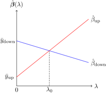
Figure 8: Equivalence between preserving the order and absence of splits relies on a simple geometrical argument.

A.2.2 The dual problem

We follow arguments developed by Tibshirani and Taylor (2011) for the generalized Lasso. Indeed, Problem (15) can be recast as

$$\,\hat{\!\boldsymbol{\beta}}(\lambda)=\mathop{\mathrm{arg\ min}}_{\boldsymbol{\beta}\in\mathbb{R}^{n}}\frac{1}{2}\left\|\mathbf{y}-\mathbf{X}\boldsymbol{\beta}\right\|_{2}^{2}+\lambda\|WD\boldsymbol{\beta}\|_{1},$$ (16)

a generalized Lasso problem with $\mathbf{X}=\mathbf{I}_{nn}$, $W$ a diagonal matrix the diagonal of which is the $n(n-1)/2$ vector given by

$$\text{diag}(W)=(w_{11},\dots,w_{1n},w_{23},\dots,w_{2n},w_{34},\dots,w_{(n-1)n})$$

and $D$ is a $n(n-1)/2\times n$ matrix that performs the pairwise differences such that

$$D=\hbox{}\vbox{\kern 0.86108pt\hbox{$\kern 0.0pt\kern 2.5pt\kern-5.0pt\left[\kern 0.0pt\kern-2.5pt\kern-5.55557pt\vbox{\kern-0.86108pt\vbox{\vbox{ \halign{\kern\arraycolsep\hfil\@arstrut$\kbcolstyle#$\hfil\kern\arraycolsep& \kern\arraycolsep\hfil$\@kbrowstyle#$\ifkbalignright\relax\else\hfil\fi\kern\arraycolsep&& \kern\arraycolsep\hfil$\@kbrowstyle#$\ifkbalignright\relax\else\hfil\fi\kern\arraycolsep\cr 5.0pt\hfil\@arstrut$\scriptstyle\text{couple }(i,j)$\hfil\kern 5.0pt&5.0pt\hfil$\scriptstyle$\hfil\kern 5.0pt&5.0pt\hfil$\scriptstyle$\hfil\kern 5.0pt&5.0pt\hfil$\scriptstyle$\hfil\kern 5.0pt&5.0pt\hfil$\scriptstyle$\hfil\kern 5.0pt&5.0pt\hfil$\scriptstyle\\(1,1)$\hfil\kern 5.0pt&5.0pt\hfil$\scriptstyle 1$\hfil\kern 5.0pt&5.0pt\hfil$\scriptstyle-1$\hfil\kern 5.0pt&5.0pt\hfil$\scriptstyle$\hfil\kern 5.0pt&5.0pt\hfil$\scriptstyle$\hfil\kern 5.0pt&5.0pt\hfil$\scriptstyle\\(1,2)$\hfil\kern 5.0pt&5.0pt\hfil$\scriptstyle 1$\hfil\kern 5.0pt&5.0pt\hfil$\scriptstyle$\hfil\kern 5.0pt&5.0pt\hfil$\scriptstyle-1$\hfil\kern 5.0pt&5.0pt\hfil$\scriptstyle$\hfil\kern 5.0pt&5.0pt\hfil$\scriptstyle\\\vdots$\hfil\kern 5.0pt&5.0pt\hfil$\scriptstyle\vdots$\hfil\kern 5.0pt&5.0pt\hfil$\scriptstyle$\hfil\kern 5.0pt&5.0pt\hfil$\scriptstyle$\hfil\kern 5.0pt&5.0pt\hfil$\scriptstyle\ddots$\hfil\kern 5.0pt&5.0pt\hfil$\scriptstyle\\(1,n)$\hfil\kern 5.0pt&5.0pt\hfil$\scriptstyle 1$\hfil\kern 5.0pt&5.0pt\hfil$\scriptstyle$\hfil\kern 5.0pt&5.0pt\hfil$\scriptstyle$\hfil\kern 5.0pt&5.0pt\hfil$\scriptstyle$\hfil\kern 5.0pt&5.0pt\hfil$\scriptstyle-1\\(2,3)$\hfil\kern 5.0pt&5.0pt\hfil$\scriptstyle$\hfil\kern 5.0pt&5.0pt\hfil$\scriptstyle 1$\hfil\kern 5.0pt&5.0pt\hfil$\scriptstyle-1$\hfil\kern 5.0pt&5.0pt\hfil$\scriptstyle$\hfil\kern 5.0pt&5.0pt\hfil$\scriptstyle\\\vdots$\hfil\kern 5.0pt&5.0pt\hfil$\scriptstyle$\hfil\kern 5.0pt&5.0pt\hfil$\scriptstyle\vdots$\hfil\kern 5.0pt&5.0pt\hfil$\scriptstyle$\hfil\kern 5.0pt&5.0pt\hfil$\scriptstyle\ddots$\hfil\kern 5.0pt&5.0pt\hfil$\scriptstyle\\(2,n)$\hfil\kern 5.0pt&5.0pt\hfil$\scriptstyle$\hfil\kern 5.0pt&5.0pt\hfil$\scriptstyle 1$\hfil\kern 5.0pt&5.0pt\hfil$\scriptstyle$\hfil\kern 5.0pt&5.0pt\hfil$\scriptstyle$\hfil\kern 5.0pt&5.0pt\hfil$\scriptstyle-1\\\vdots$\hfil\kern 5.0pt&5.0pt\hfil$\scriptstyle$\hfil\kern 5.0pt&5.0pt\hfil$\scriptstyle$\hfil\kern 5.0pt&5.0pt\hfil$\scriptstyle$\hfil\kern 5.0pt&5.0pt\hfil$\scriptstyle$\hfil\kern 5.0pt&5.0pt\hfil$\scriptstyle\\(n-1,n)$\hfil\kern 5.0pt&5.0pt\hfil$\scriptstyle$\hfil\kern 5.0pt&5.0pt\hfil$\scriptstyle$\hfil\kern 5.0pt&5.0pt\hfil$\scriptstyle$\hfil\kern 5.0pt&5.0pt\hfil$\scriptstyle 1$\hfil\kern 5.0pt&5.0pt\hfil$\scriptstyle-1\\$\hfil\kern 5.0pt\crcr}}}}\right]$}}.$$ (17)

In what follows, it will be convenient to index rows of the matrix $D$ in terms of the couple $(i,j)$, as is done in Expression (17).

We then rely on the Lagrangian dual of the primal problem (16) studied in Tibshirani and Taylor (2011), which is

$$\hat{\mathbf{u}}(\lambda)=\mathop{\mathrm{arg\ min}}_{\mathbf{u}\in\mathbb{R}^{(n(n-1)/2)}}\frac{1}{2}\left\|\mathbf{y}-D^{T}W\mathbf{u}\right\|_{2}^{2}\quad\text{subject to }\|\mathbf{u}\|_{\infty}\leq\lambda,$$ (18)

and where the correspondence between the primal and dual variables is

$$\,\hat{\!\boldsymbol{\beta}}=\mathbf{y}-D^{T}W\hat{\mathbf{u}}.$$

The dual solution must satisfies

$$\hat{u}_{ij}\in\begin{cases}\left\{+\lambda\right\}&\text{ if }(WD\,\hat{\!\boldsymbol{\beta}})_{ij}>0,\\ \left\{-\lambda\right\}&\text{ if }(WD\,\hat{\!\boldsymbol{\beta}})_{ij}<0,\\ [-\lambda,+\lambda]&\text{ if }(WD\,\hat{\!\boldsymbol{\beta}})_{ij}=0,\\ \end{cases}$$

where we use the indexing in terms of $(i,j)$ for the vector $\mathbf{u}$. We also define $\mathcal{B}$, the set of $(i,j)$ such that $|u_{ij}|=\lambda$, that is, the ones reaching the boundary in the dual.

The key point is to note that the order is not preserved if and only if, at some point of the path, there exists some $(i,j)$ and $\lambda$ such that $\hat{u}_{ij}(\lambda)=-\lambda$, meaning that $(WD\beta)_{ij}<0$. The rest of the proof will show that this event is not possible for distance decreasing weights and the matrix $D$ given by (17). To this end, we proceed by contradiction, by supposing that the order is not preserved along the path. We thus consider the first split event that will disrupt the order, which occurs at $\lambda_{0}$. At this point, the order is preserved and there is an $\varepsilon>0$ such that on $]\lambda_{0},\lambda_{0}+\varepsilon]$, the order is not preserved. We note that $\lambda_{0}>0$ since the order is necessarily preserved up to the first fusion event that fuses data points with different values. At $\lambda_{0}$, we must have a couple $(i^{0},j^{0})$ such that $\hat{u}_{i^{0}j^{0}}(\lambda_{0})=-\lambda_{0}$ that reaches the boundary. Moreover, the left derivative $\partial^{-}\hat{u}_{i^{0}j^{0}}(\lambda)$ must be less than $-1$ because the path is continuous (see Tibshirani and Taylor, 2011) and because we consider the first event disrupting the order. We provide geometrical insight into this point on Figure 9.

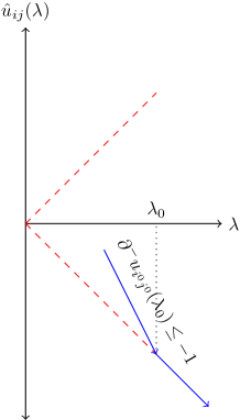
Figure 9: Geometrical insight into a split event in the dual.

We now show that we necessarily have $\partial^{-}\hat{u}_{i^{0}j^{0}}(\lambda)>-1$, leading to a contradiction. To this end, we consider the set $\mathcal{C}$ of indices which are fused with $i^{0}$ and $j^{0}$ just before $\lambda_{0}$, that is, $\mathcal{C}=\left\{i:\hat{\beta}_{i}=\hat{\beta}_{i^{0}}=\hat{\beta}_{j^{0}}\right\}$. We denote by

$$\mathcal{D}_{\text{in}}=\left\{(i,j)\in\mathcal{C}\times\mathcal{C}:i<j\right\}$$

the set of intra $\mathcal{C}$ differences and

$$\mathcal{D}_{\text{out}}=\left\{(i,j)\in\mathcal{B}:i<j,i\in\mathcal{C}\text{ or }j\in\mathcal{C}\right\},$$

the set of differences between $\mathcal{C}$ and other groups. Finally we denote by $\mathcal{R}$ the set of all other indices which are not in $\mathcal{D}_{\text{out}}$ and $\mathcal{D}_{\text{in}}$. Given those sets we reindex the matrix $D$ and $W$ as follows.

$$D=\hbox{}\vbox{\kern 0.86108pt\hbox{$\kern 0.0pt\kern 2.5pt\kern-5.0pt\left[\kern 0.0pt\kern-2.5pt\kern-5.55557pt\vbox{\kern-0.86108pt\vbox{\vbox{ \halign{\kern\arraycolsep\hfil\@arstrut$\kbcolstyle#$\hfil\kern\arraycolsep& \kern\arraycolsep\hfil$\@kbrowstyle#$\ifkbalignright\relax\else\hfil\fi\kern\arraycolsep&& \kern\arraycolsep\hfil$\@kbrowstyle#$\ifkbalignright\relax\else\hfil\fi\kern\arraycolsep\cr 5.0pt\hfil\@arstrut$\scriptstyle\text{set of index }$\hfil\kern 5.0pt&5.0pt\hfil$\scriptstyle\mathcal{C}$\hfil\kern 5.0pt&5.0pt\hfil$\scriptstyle\bar{\mathcal{C}}\\\mathcal{D}_{\text{in}}$\hfil\kern 5.0pt&5.0pt\hfil$\scriptstyle D_{\mathcal{D}_{\text{in}}\times\mathcal{C}}$\hfil\kern 5.0pt&5.0pt\hfil$\scriptstyle D_{\mathcal{D}_{\text{in}}\times\bar{\mathcal{C}}}\\\mathcal{D}_{\text{out}}$\hfil\kern 5.0pt&5.0pt\hfil$\scriptstyle D_{\mathcal{D}_{\text{out}}\times\mathcal{C}}$\hfil\kern 5.0pt&5.0pt\hfil$\scriptstyle D_{\mathcal{D}_{\text{out}}\times\bar{\mathcal{C}}}\\\mathcal{R}$\hfil\kern 5.0pt&5.0pt\hfil$\scriptstyle D_{\mathcal{R}\times\mathcal{C}}$\hfil\kern 5.0pt&5.0pt\hfil$\scriptstyle D_{\mathcal{R}\times\bar{\mathcal{C}}}\\$\hfil\kern 5.0pt\crcr}}}}\right]$}}$$

$$W=\hbox{}\vbox{\kern 0.86108pt\hbox{$\kern 0.0pt\kern 2.5pt\kern-5.0pt\left[\kern 0.0pt\kern-2.5pt\kern-5.55557pt\vbox{\kern-0.86108pt\vbox{\vbox{ \halign{\kern\arraycolsep\hfil\@arstrut$\kbcolstyle#$\hfil\kern\arraycolsep& \kern\arraycolsep\hfil$\@kbrowstyle#$\ifkbalignright\relax\else\hfil\fi\kern\arraycolsep&& \kern\arraycolsep\hfil$\@kbrowstyle#$\ifkbalignright\relax\else\hfil\fi\kern\arraycolsep\cr 5.0pt\hfil\@arstrut$\scriptstyle\text{set of index }$\hfil\kern 5.0pt&5.0pt\hfil$\scriptstyle\mathcal{D}_{\text{in}}$\hfil\kern 5.0pt&5.0pt\hfil$\scriptstyle\mathcal{D}_{\text{out}}$\hfil\kern 5.0pt&5.0pt\hfil$\scriptstyle\mathcal{R}\\\mathcal{D}_{\text{in}}$\hfil\kern 5.0pt&5.0pt\hfil$\scriptstyle W_{\mathcal{D}_{\text{in}}^{2}}$\hfil\kern 5.0pt&5.0pt\hfil$\scriptstyle 0$\hfil\kern 5.0pt&5.0pt\hfil$\scriptstyle 0\\\mathcal{D}_{\text{out}}$\hfil\kern 5.0pt&5.0pt\hfil$\scriptstyle 0$\hfil\kern 5.0pt&5.0pt\hfil$\scriptstyle W_{\mathcal{D}_{\text{out}}^{2}}$\hfil\kern 5.0pt&5.0pt\hfil$\scriptstyle 0\\\mathcal{R}$\hfil\kern 5.0pt&5.0pt\hfil$\scriptstyle 0$\hfil\kern 5.0pt&5.0pt\hfil$\scriptstyle 0$\hfil\kern 5.0pt&5.0pt\hfil$\scriptstyle W_{\mathcal{R}^{2}}\\$\hfil\kern 5.0pt\crcr}}}}\right]$}}$$

By definition, for all $(i,j)\in\mathcal{R}$, $i$ and $j$ do not belong to $\mathcal{C}$ and thus $D_{\mathcal{R}\times\mathcal{C}}=0$. By simple matrix algebra, the restriction of $D^{T}W$ to the rows in $\mathcal{C}$ can be written

$$(D^{T}W)_{\mathcal{C}}=(D_{\mathcal{D}_{\text{in}}\times\mathcal{C}})^{T}W_{\mathcal{D}_{\text{in}}^{2}}+(D_{\mathcal{D}_{\text{out}}\times\mathcal{C}})^{T}W_{\mathcal{D}_{\text{out}}^{2}}.$$

Just before $\lambda_{0}$ and for all $(i,j)\in\mathcal{D}_{\text{out}}$, we have $\hat{u}_{ij}(\lambda)=\lambda$ and so $\text{sign}(\hat{u}_{ij})=1$, because the order is preserved at this point. Then, following Tibshirani and Taylor (2011), the KKT conditions of (18) restricted to $\mathcal{D}_{\text{in}}$ imply that

$$\hat{\mathbf{u}}_{\mathcal{D}_{\text{in}}}(\lambda)=\\ \left(W_{\mathcal{D}_{\text{in}}^{2}}D_{\mathcal{D}_{\text{in}}\times\mathcal{C}}D_{{\mathcal{D}_{\text{in}}\times\mathcal{C}}}^{T}W_{\mathcal{D}_{\text{in}}^{2}}\right)^{+}W_{\mathcal{D}_{\text{in}}^{2}}D_{{\mathcal{D}_{\text{in}}\times\mathcal{C}}}\left(\mathbf{y}-\lambda(W_{\mathcal{D}_{\text{out}}^{2}}D_{{\mathcal{D}_{\text{out}}\times\mathcal{C}}})^{T}\mathbf{1}_{\mathcal{D}_{\text{out}}}\right),$$ (19)

where $A^{+}$ denotes the Moore-Penrose pseudo-inverse of $A$. Note that such a choice is important since it guarantees that $\hat{\mathbf{u}}(\lambda)$ is a continuous function of $\lambda$.

Expression of (19) greatly simplifies by exploiting an explicit formula for the pseudo-inverse, which we derive in the next paragraph.

Analytic form of the pseudo-inverse.

In this paragraph, we consider only the $D_{\mathcal{D}_{\text{in}}\times\mathcal{C}}$ matrix and the $W_{\mathcal{D}_{\text{in}}^{2}}$ matrix, which correspond to the set of intra $\mathcal{C}$ differences and their weights. For simplicity, we just denote them $D$ and $W$ here and call $n^{\prime}$ the group size. We have

$$D^{T}D=n^{\prime}\mathbf{I}_{n^{\prime}n^{\prime}}-\mathbf{1}_{n^{\prime}}\mathbf{1}_{n^{\prime}}^{T},\quad D\mathbf{1}_{n^{\prime}}=\mathbf{0}_{n^{\prime}},$$

and from this we get $DD^{T}D=n^{\prime}D$ and thus, $D^{+}=D^{T}/n^{\prime}$. Finally

$$(DD^{T})^{+}=\frac{1}{{n^{\prime}}^{2}}DD^{T},\quad\text{ and }(DD^{T})^{+}D=\frac{D}{n^{\prime}}.$$

If we now consider the weighted version of Problem (16), one has

$$(WDD^{T}W)^{+}WD=W^{-1}(DD^{T})^{+}W^{-1}WD=\frac{W^{-1}D}{n^{\prime}}.$$

Back to our problem,

Expression (19) becomes

$$\hat{\mathbf{u}}_{\mathcal{D}_{\text{in}}}(\lambda)=\frac{1}{n_{\mathcal{C}}}W_{\mathcal{D}_{\text{in}}^{2}}^{-1}D_{\mathcal{D}_{\text{in}}\times\mathcal{C}}\left(\mathbf{y}-\lambda\underbrace{(W_{\mathcal{D}_{\text{out}}^{2}}D_{{\mathcal{D}_{\text{out}}\times\mathcal{C}}})^{T}\mathbf{1}_{\mathcal{D}_{\text{out}}}}_{V}\right).$$ (20)

Let us consider the size-$n_{\mathcal{C}}$ vector $V$, which includes the differences between elements in $\mathcal{C}$ and elements outside $\mathcal{C}$. Note that the $i$th column of $D_{{\mathcal{D}_{\text{out}}\times\mathcal{C}}}$ is zero everywhere, except for the elements of $\mathcal{D}_{\text{out}}$ containing $i$. In the last case, it is equal to $1$ if $y_{i}\geq y_{j}$ and to $-1$ otherwise. Hence,

$$V_{i}=\left((D_{{\mathcal{D}_{\text{out}}\times\mathcal{C}}})^{T}W_{\mathcal{D}_{\text{out}}^{2}}\mathbf{1}_{\mathcal{D}_{\text{out}}}\right)_{i}=\sum_{j\in\bar{\mathcal{C}}}w_{ij}\mathrm{sign}(y_{i}-y_{j}).$$

Also recall that the matrix $D_{\mathcal{D}_{\text{in}}\times\mathcal{C}}$ encodes the pairwise positive differences. Then for $y_{i}>y_{i^{\prime}}$, the $(i,i^{\prime})$ element of $D_{\mathcal{D}_{\text{in}}\times\mathcal{C}}V$ equals

$$(D_{\mathcal{D}_{\text{in}}\times\mathcal{C}}V)_{ii^{\prime}}=V_{i}-V_{i^{\prime}}=\sum_{j\in\bar{\mathcal{C}}}w_{ij}\mathrm{sign}(y_{i}-y_{j})-w_{i^{\prime}j}\mathrm{sign}(y_{i^{\prime}}-y_{j}).$$

There are two possibilities: either $y_{j}>y_{i}\geq y_{i^{\prime}}$ or $y_{i}\geq y_{i^{\prime}}>y_{j}$. We thus split the summation in the above equation into two parts:

$$(D_{\mathcal{D}_{\text{in}}\times\mathcal{C}}V)_{ii^{\prime}}=\sum_{\begin{subarray}{c}j\in\bar{\mathcal{C}}\\ y_{j}>y_{i}\geq y_{i^{\prime}}\end{subarray}}(w_{i^{\prime}j}-w_{ij})+\sum_{\begin{subarray}{c}j\in\bar{\mathcal{C}}\\ y_{i}\geq y_{i^{\prime}}>y_{j}\end{subarray}}(w_{ij}-w_{i^{\prime}j}).$$

And from this we see that if the weights are positive and distance decreasing, all the $(D_{\mathcal{D}_{\text{in}}\times\mathcal{C}}V)_{ii^{\prime}}$ are negative. To conclude, the slopes in Expression (20), that is,

$$-\frac{\lambda}{n_{\mathcal{C}}}W_{\mathcal{D}_{\text{in}}^{2}}^{-1}D_{\mathcal{D}_{\text{in}}\times\mathcal{C}}(W_{\mathcal{D}_{\text{out}}^{2}}D_{{\mathcal{D}_{\text{out}}\times\mathcal{C}}})^{T}\mathbf{1}_{\mathcal{D}_{\text{out}}}$$

are positive, which is in contradiction with $\partial^{-}\hat{u}_{i^{0}j^{0}}(\lambda)\leq-1$.

A.3 Theorem 3: consistency for exponentially adaptive weights

We essentially follow the same line as for the adaptive Lasso in Zou (2006), yet adapted to the fusion penalty as in Viallon et al. (2014); Bondell and Reich (2008b). The main difference comes from the use of the exponentially adaptive weights $w_{k\ell}^{\text{FA}}$.

We start by asymptotics in the vein of Fu and Knight (2001) for Lasso-type procedures: Lemma 3 below gives the limiting distribution of the fused-ANOVA estimator (12) on the range of interest for the penalty $\lambda_{n}$ which essentially proves the asymptotic normality part of the Theorem.

Lemma 3.

Suppose $\lambda_{n}n^{3/2}\exp\left\{-\alpha\sqrt{n}\right\}\to 0$ and $\lambda_{n}n^{3/2}\to\infty$. Then,

$$\sqrt{n}(\,\hat{\!\boldsymbol{\beta}}^{(n)}-\boldsymbol{\beta}^{\star})\xrightarrow{d}\mathop{\mathrm{arg\ min}}_{\mathbf{u}}V(\mathbf{u}),$$

where, for $\mathbf{W}\sim\mathcal{N}(\mathbf{0},\sigma^{2}\mathbf{D})$,

$$V(\mathbf{u})=\begin{cases}-2\mathbf{u}^{T}\mathbf{W}+\mathbf{u}^{T}\mathbf{D}\mathbf{u}&\text{if $u_{k}=u_{\ell}$ for all $(k,\ell)\in\mathcal{A}^{\star}$}\\ \infty&\text{otherwise.}\\ \end{cases}$$

Proof.

Let $\,\hat{\!\boldsymbol{\beta}}^{(n)}=\boldsymbol{\beta}^{\star}+\frac{\mathbf{u}_{n}}{\sqrt{n}}$ – or equivalently $\mathbf{u}_{n}=\sqrt{n}(\,\hat{\!\boldsymbol{\beta}}^{(n)}-\boldsymbol{\beta}^{\star})$ – where $\boldsymbol{\beta}^{\star}$ is the true vector of parameters and $\mathbf{u}_{n}=\mathop{\mathrm{arg\ min}}_{\mathbf{u}\in\mathbb{R}^{K}}\Phi_{n}(\mathbf{u})$ with

$$\Phi_{n}(\mathbf{u})=\frac{1}{2}\sum_{k=1}^{K}n_{k}\left(y_{i}-(\beta^{\star}_{k}+\frac{u_{k}}{\sqrt{n}})\right)^{2}+\lambda_{n}\ \sum_{k\neq\ell}w_{k\ell}^{\text{FA}}\left|\beta^{\star}_{k}-\beta^{\star}_{\ell}+\frac{u_{k}-u_{\ell}}{\sqrt{n}}\right|.$$

Note that $\mathbf{u}_{n}$ is also the minimizer of $V_{n}(\mathbf{u})=\Phi_{n}(\mathbf{u})-\Phi(\mathbf{0})$ which is written

$$V_{n}(\mathbf{u})=\sum_{k}\frac{n_{k}}{n}u_{k}^{2}-2\sum_{k}\frac{n_{k}}{n}\varepsilon_{k}+\frac{\lambda_{n}}{\sqrt{n}}\sum_{k,\ell}w_{k\ell}^{\text{FA}}\underbrace{\sqrt{n}\left(\left|\beta^{\star}_{k}-\beta_{\ell}^{k}+\frac{u_{k}-u_{\ell}}{\sqrt{n}}\right|-\left|\beta^{\star}_{k}-\beta_{\ell}^{\star}\right|\right)}_{T_{k\ell}^{(n)}}.$$

Let us study the limiting behavior of $V_{n}$. The basic assumptions for our fused-ANOVA Problem (12) are having a design such that $\lim_{n\to\infty}n_{k}/n=\rho_{k}$ and having i.i.d residuals with zero mean and common variance $\sigma^{2}$. Thus, the first two terms in $V_{n}$ respectively converge to a constant $\mathbf{u}^{T}\mathbf{D}\mathbf{u}$ and to a Gaussian $\mathbf{W}=\mathcal{N}(\mathbf{0},\sigma^{2}\mathbf{D})$, where $\mathbf{D}$ is a $K$-diagonal matrix such as $D_{kk}=\rho_{k}$. For the third term, there are two possibilities: either $\beta^{\star}_{k}=\beta_{\ell}^{\star}$ or $\beta^{\star}_{k}\neq\beta_{\ell}^{\star}$. In other words, $(k,\ell)$ belongs to $\mathcal{A}^{\star}$ or does not. First note that

$$T_{k\ell}^{(n)}\xrightarrow[]{n\to\infty}\begin{cases}|u_{k}-u_{\ell}|&\text{if }(k,\ell)\in\mathcal{A}^{\star},\\ (u_{k}-u_{\ell})\mathrm{sign}(\beta_{k}^{\star}-\beta_{\ell}^{\star})&\text{otherwise}.\end{cases}$$

In words, this part of the third term converges to a finite constant in both situations which is null as soon as $u_{k}=u_{\ell}$. Second, consider the remaining part of this third term which involves the weights $w_{k\ell}^{\text{FA}}$. It suffices to use the $\sqrt{n}$-consistency of the OLS estimators $(\bar{y}_{1},\dots,\bar{y}_{K})$ coupled with assumptions made on the limiting behavior of $\lambda_{n}$ to see that

$$\frac{\lambda_{n}}{\sqrt{n}}w_{k\ell}^{\text{FA}}=\frac{\lambda_{n}}{\sqrt{n}}n_{k}n_{\ell}\exp\left\{-\alpha\sqrt{n}|\bar{y}_{k}-\bar{y}_{\ell}|\right\}\to\begin{cases}\infty&\text{if }(k,\ell)\in\mathcal{A}^{\star},\\ 0&\text{otherwise}.\end{cases}$$

Application of Slutsky’s Lemma gives the limiting behavior of the third term in $V_{n}$ and we finally get $V_{n}(\mathbf{u})\to V(\mathbf{u})$ with $V$ defined as in Lemma 3.

The final convergence of $\mathbf{u}_{n}\to_{d}\mathop{\mathrm{arg\ min}}_{\mathbf{u}}V(\mathbf{u})$ is obtained by applying epi-convergence results of Geyer (1994). ∎

Turning back to the proof of Theorem 3, just note that the unique minimizer of the convex function $V(\mathbf{u})$ in Lemma 3 is $\mathbf{u}^{\star}=\mathbf{D}^{-1}\mathbf{W}\sim\mathcal{N}(\mathbf{0},\sigma^{2}\mathbf{D}^{-1})$ such that $u^{\star}_{k}=u^{\star}_{\ell}$ for all $(k,\ell)\in\mathcal{A}^{\star}$ and the asymptotic normality part is proved.

We now proceed to the consistency in terms of support recovery. First, concerning the elements of $\,\hat{\!\boldsymbol{\beta}}$ that should not fuse according to the true $\mathcal{A}^{\star}$, Lemma 3 indicates that

$$\mathbb{P}\left((k,\ell)\notin\hat{\mathcal{A}}_{n}|(k,\ell)\notin\mathcal{A}^{\star}\right)=1-\mathbb{P}\left(\hat{\beta}_{k}^{(n)}=\hat{\beta}^{(n)}_{\ell}|\beta_{k}^{\star}\neq\beta_{\ell}^{\star}\right)\to 1.$$

Second, regarding elements of $\hat{\beta}$ that must fuse, we need to prove that

$$\mathbb{P}\left((k,\ell)\in\hat{\mathcal{A}}_{n}|(k,\ell)\in\mathcal{A}^{\star}\right)=\mathbb{P}\left(\hat{\beta}_{k}^{(n)}=\hat{\beta}^{(n)}_{\ell}|\beta_{k}^{\star}=\beta_{\ell}^{\star}\right)\to 1.$$

To this end, we proceed as in Viallon et al. (2014) to get a contradiction by considering the largest $\hat{\beta}_{k^{\prime}}$ such that $\hat{\beta}_{k}\neq\hat{\beta}_{\ell}$ even though $\beta_{k}^{\star}=\beta_{\ell}^{\star}$. This can be done by inspecting the KKT conditions asymptotically. In the univariate case and for $\Omega$ the $\ell_{1}$-norm, an optimal $\hat{\beta}$ verifies the following subgradient equation for all $k=1,\dots,K$. This is written

$$\frac{n_{k}}{\sqrt{n}}(\hat{\beta}_{k}-\bar{y}_{k})=\frac{\lambda_{n}}{\sqrt{n}}\sum_{\begin{subarray}{c}\ell:\ell\neq k\\ (k,\ell)\in\mathcal{A}^{\star}\end{subarray}}w_{k\ell}^{\text{FA}}\tau_{k\ell}+\frac{\lambda_{n}}{\sqrt{n}}\sum_{\begin{subarray}{c}\ell:\ell\neq k\\ (k,\ell)\notin\mathcal{A}^{\star}\end{subarray}}w_{k\ell}^{\text{FA}}\mathrm{sign}\left(\hat{\beta}_{k}-\hat{\beta}_{\ell}\right).$$ (21)

Now, in the first term of the right-hand side, suppose that there exists at least one $\ell$ such that $(k,\ell)\in\mathcal{A}^{\star}$ and $\hat{\beta}_{k}\neq\hat{\beta}_{\ell}$ simultaneously; consider $\hat{\beta}_{k^{\prime}}$ with $k^{\prime}=\mathop{\mathrm{arg\ max}}_{\ell:(k,\ell)\in\mathcal{A}^{\star}}\{\hat{\beta}_{\ell}\}$, the largest coefficients verifying these conditions: we must have $\tau_{k^{\prime}\ell}=1$ for all $\ell$ such that $\hat{\beta}_{\ell}\neq\hat{\beta}_{k^{\prime}}$ and $\beta_{\ell}^{\star}=\beta_{k^{\prime}}^{\star}$. Now if we sum equation (21) for all $\ell$ that are fused with $k^{\prime}$ we obtain:

$$\sum_{\ell|\hat{\beta}_{\ell}=\hat{\beta}_{k^{\prime}}}\frac{n_{\ell}}{\sqrt{n}}(\hat{\beta}_{k^{\prime}}-\bar{y}_{\ell})=\frac{\lambda_{n}}{\sqrt{n}}\sum_{\ell|\hat{\beta}_{\ell}=\hat{\beta}_{k^{\prime}}}\ \sum_{\begin{subarray}{c}k|(k,\ell)\in\mathcal{A}^{\star}\\ \cap\ \hat{\beta}_{k}\neq\hat{\beta}_{k^{\prime}}\end{subarray}}w_{k\ell}^{\text{FA}}\\ +\frac{\lambda_{n}}{\sqrt{n}}\sum_{\ell|\hat{\beta}_{\ell}=\hat{\beta}_{k^{\prime}}}\ \sum_{\begin{subarray}{c}\ell:\ell\neq k\\ (k,\ell)\notin\mathcal{A}^{\star}\end{subarray}}w_{k\ell}^{\text{FA}}\mathrm{sign}\left(\hat{\beta}_{k}-\hat{\beta}_{\ell}\right).$$ (22)

By Lemma 3 and asymptotic normality, the left-hand side in (22) converges to a $\mathcal{O}_{P}(1)$. Then, the second term on the right-hand side (that is, elements that should not fuse) tends to $0$ since $\lambda_{n}w_{k\ell}^{\text{FA}}/\sqrt{n}\to 0$ when $(k,\ell)\notin\mathcal{A}^{\star}$, as seen previously. Finally we have :

$$\frac{\lambda_{n}}{\sqrt{n}}\sum_{\ell|\hat{\beta}_{\ell}=\hat{\beta}_{k^{\prime}}}\ \sum_{\begin{subarray}{c}k|(k,\ell)\in\mathcal{A}^{\star}\\ \cap\ \hat{\beta}_{k}\neq\hat{\beta}_{k^{\prime}}\end{subarray}}w_{k\ell}^{\text{FA}}\xrightarrow[]{n\to\infty}\infty$$

which is in contradiction with the rest of the subgradient equation of $\beta_{k^{\prime}}$ since we recall that the left-hand side is $\mathcal{O}_{P}(1)$. Therefore we must have $\mathbb{P}\left((k,\ell)\in\hat{\mathcal{A}}_{n}\right)\to 1$ for all $(k,\ell)\in\mathcal{A}^{\star}$, which completes the proof of the consistency part in Theorem 3.

References

- Bondell and Reich (2008a) H. D. Bondell and B. J. Reich. Simultaneous regression shrinkage, variable selection, and supervised clustering of predictors with OSCAR. Biometrics, 64(1):115–123, 2008a.
- Bondell and Reich (2008b) H.D. Bondell and B.J. Reich. Simultaneous factor selection and collapsing levels in ANOVA. Biometrics, 65(1):169–177, 2008b.
- Boyd and Vandenberghe (2004) S.P. Boyd and L. Vandenberghe. Convex optimization. Cambridge Universuity Press, 2004.
- Efron et al. (2004) B. Efron, T. Hastie, I. Johnstone, and R. Tibshirani. Least angle regression. Ann. Statist., 32(2):407–499, 2004.
- Fan and Li (2001) J. Fan and R. Li. Variable Selection via Nonconcave Penalized Likelihood and Its Oracle Properties. JASA, 96(456):1348–1360, 2001.
- Friedman et al. (2007) Jerome Friedman, Trevor Hastie, Holger Höfling, Robert Tibshirani, et al. Pathwise coordinate optimization. The Annals of Applied Statistics, 1(2):302–332, 2007.
- Fu and Knight (2001) W. Fu and K. Knight. Asymptotics for lasso-type estimators. Ann. Statist., 28(5):1245–1501, 2001.
- Gertheiss and Tutz (2010) Jan Gertheiss and Gerhard Tutz. Sparse modeling of categorial explanatory variables. The Annals of Applied Statistics, pages 2150–2180, 2010.
- Geyer (1994) C.J. Geyer. Simultaneous factor selection and collapsing levels in ANOVA. Ann. Statist., 22(4):1635–2134, 1994.
- Hocking et al. (2011) T. Hocking, J.-P. Vert, F. Bach, and A. Joulin. Clusterpath: an algorithm for clustering using convex fusion penalties. In Proceedings of the 28th ICML, pages 745–752, 2011.
- Hoefling (2010) H. Hoefling. A path algorithm for the fused lasso signal approximator. J. Comput. Graph. Statist., 19(4):984–1006, 2010.
- Mairal and Yu (2012) J. Mairal and B. Yu. Complexity analysis of the lasso regularization path. In Proceedings of the 29th ICML, 2012.
- Rosset and Zhu (2007) S. Rosset and J. Zhu. Piecewise linear regularized solution paths. Ann. Statist., 35(3):1012–1030, 2007.
- Tibshirani and Taylor (2011) R. J. Tibshirani and J. Taylor. The solution path of the generalized lasso. Ann. Statist., 39(3):1335–1371, 2011.
- Vetrovsky and Baldrian (2013) Tomas Vetrovsky and Petr Baldrian. The variability of the 16S rRNA gene in bacterial genomes and its consequences for bacterial community analyses. PLoS ONE, 8(2):e57923, 2013. doi: 10.1371/journal.pone.0057923.
- Viallon et al. (2014) Vivian Viallon, Sophie Lambert-Lacroix, Hölger Hoefling, and Franck Picard. On the robustness of the generalized fused lasso to prior specifications. Statistics and Computing, pages 1–17, 2014.
- Zou (2006) H. Zou. The adaptive lasso and its oracle properties. JASA, 101(476):1418–1429, 2006.