Device-independent tomography of multipartite quantum states

Abstract

In the usual tomography of multipartite entangled quantum states one assumes that the measurement devices used in the laboratory are under perfect control of the experimenter. In this paper, using the so-called SWAP concept introduced recently, we show how one can remove this assumption in realistic experimental conditions and nevertheless be able to characterize the produced multipartite state based only on observed statistics. Such a black box tomography of quantum states is termed self-testing. As a function of the magnitude of the Bell violation, we are able to self-test emblematic multipartite quantum states such as the three-qubit W state, the three- and four-qubit Greenberger-Horne-Zeilinger states, and the four-qubit linear cluster state.

I Introduction

Quantum entanglement rmp_horo plays a prominent role in quantum theory, and particularly in quantum information. Indeed, a big effort has been devoted to its characterization and detection recently review_toth .

In usual tomography of entangled quantum states, one has to rely on certain assumptions about the measurement devices used in the experiment. These assumptions are usually difficult to meet in practice. For instance, the characterization of a quantum state cannot be considered conclusive if the devices implementing the specific measurement operators are not under precise control of the experimenter rosset .

In the last years, the experimental preparation of complex multipartite states has become a routine. State of the art photonic experiments can generate and characterize six-qubit entangled states photonic ; pistate . More recently, 14 entangled qubits were generated in ion-trap experiments monz ; lanyon . Such is the range of qubits, for which, in order to do a full tomography and reconstruct completely the produced multipartite state, one has to resort to additional information about the state. Such additional knowledge has been exploited in the literature for states of low rank gross , for a matrix product state mps or for a permutationally invariant (PI) state pistate . Although these extra assumptions may simplify the analysis considerably, the characterization of the quantum state usually becomes less accurate.

In this paper, we follow a different approach based on the so-called device-independent paradigm (see review_scarani for a review), which regards the local systems as black boxes with some input and outputs and is minimalist in the sense that it requires only the no-signalling assumption and that inputs are freely chosen.

Tomography of quantum states in this device-independent framework, where one characterizes multipartite states based only on lists of statistical data coming from a Bell-type experiment, was termed self-testing in the seminal work of Mayers and Yao my . At that time the task of self-testing was mostly applied in the ideal situation (see pioneering works in Refs. selftest_ideal as well). Later, this limitation has been removed and since then a number of works selftest_nonideal have demonstrated self-testing robust to external noise. However, the noise to be tolerated in these schemes was extremely small. A resolution to this issue was given by Ref. swap , which could extend self-testing of quantum states and measurement devices to realistic experimental situations. As an illustration of the power of the so-called SWAP method of swap , it has been proved in the bipartite case that a CHSH chsh violation of $2.57$ certifies a singlet fidelity of more than $70\%$.

In this paper, making use of the SWAP method, we move from the bipartite to the multipartite domain by self-testing famous multipartite states such as the W state dur , the $3\&4$-qubit Greenberger-Horne-Zeilinger (GHZ) states ghz , and the 4-qubit cluster state cluster (recall that each of these states has been implemented in the lab in photonic experiments about a decade ago w_exp ,ghz_exp ,cluster_exp ). Note that in our task of self-testing we do not assume any knowledge regarding the specific workings of the experimental devices (such as the dimension of the underlying Hilbert spaces or the type of measurements involved), however, we accept that quantum theory holds exactly.

To this end, we introduce the framework of Bell nonlocality tests. Consider three distant observers, Alice, Bob, and Cecil, and allow each of them to choose freely between two ($i=1,2$) dichotomic observables, $A_{i}=\pm 1$, $B_{i}=\pm 1$, and $C_{i}=\pm 1$, respectively. In a specific run of the experiment, the correlations between the observations can be represented by the product of the type $A_{i}B_{j}C_{k}$. The correlation function is then the average over many runs of the experiment $\langle A_{i}B_{j}C_{k}\rangle$ for $i,j,k=0,1,2$ (where we have chosen $A_{0}=B_{0}=C_{0}=1$ to account for subcorrelation terms). In quantum mechanics, the above mean value can be calculated as follows:

$$\langle A_{i}B_{j}C_{k}\rangle=\mbox{tr}\left(\rho\cdot\hat{A_{i}}\otimes\hat{B_{j}}\otimes\hat{C_{k}}\right),$$ (1)

where $\rho$ denotes Alice, Bob and Cecil’s tripartite state, and we have set $\hat{A_{0}}=\hat{B_{0}}=\hat{C_{0}}=\leavevmode\hbox{\small 1\normalsize\kern-3.30002pt1}$.

Note: we never use the fact that the underlying black box state is pure. And we shouldn’t, because, in that case, we just have to show correlation in order to prove entanglement. We do assume, however, that measurements are projective.

Remarkably, there exist situations in this setting where the observed statistics $\{\langle A_{i}B_{j}C_{k}\rangle\}_{i,j,k}$ suffice to determine the underlying state $|\bar{\psi}\rangle$ and observables $\bar{A}_{i},\bar{B}_{j},\bar{C}_{k}$, up to local isometries and some additional (but irrelevant) degrees of freedom. For instance, let us consider the following famous set of correlations

$$\langle A_{1}B_{1}C_{1}\rangle=1,$$

$$\langle A_{1}B_{2}C_{2}\rangle=\langle A_{2}B_{1}C_{2}\rangle=\langle A_{2}B_{2}C_{1}\rangle=-1,$$ (2)

exhibiting the so-called GHZ paradox ghz ,merminpara . It has been shown recently that the only state compatible with these correlations is the famous GHZ state (up to local isometries and adding local ancillary systems to the state) mckague . However, in realistic experimental conditions, we cannot hope that the above averages attain $\pm 1$ exactly. In order to quantify how close the actual state in the box $\rho\in B(\mathcal{H}_{box})$ is to our mathematical guess $|\bar{\psi}\rangle\in\mathbb{C}^{d}$, we must hence introduce a figure of merit. A quite significant one is the fidelity modulo local isometries, defined as

$$F=\max_{U}\langle\bar{\psi}|\mbox{tr}_{junk}(U\rho U^{\dagger})|\bar{\psi}\rangle.$$ (3)

Here the “junk” system denotes extra degrees of freedom which are not necessary -in first approximation- to capture the physics of the experiment, and the maximization is performed over all local isometries $U:\mathcal{H}_{box}\to\mathbb{C}^{d}\otimes\mathcal{H}_{junk}$.

Our task is to estimate the minimal value of the fidelity $F$ compatible with the observed statistics $\{\langle A_{i}B_{j}C_{k}\rangle\}_{i,j,k}$ (note that $F=1$ with respect to some reference state $|\bar{\psi}\rangle$ implies perfect self-testing). For didactic purposes, in this work we will not discuss self-testing criteria which require the knowledge of the whole set of correlations. Rather, we will investigate how the fidelity $F$ with respect to multipartite (three-qubit and four-qubit) states varies as a function of the magnitude of violation of specific Bell inequalities. This will be possible thanks to the recently developed SWAP method swap .

Let us mention some recent works in the spirit of our paper, where information regarding the state produced could be extracted from multipartite Bell experiments: In Ref. gme , genuine multipartite entanglement could be detected from Bell-type inequalities, which test was implemented experimentally as well recently gmeexp . Another promising method was proposed by Moroder et al. moroder , which method provides access to certain properties of a composite system via Bell inequalities, such as negativity neg and can be extended to the multipartite realm (see also structure for related results). Finally, we would like to call the attention of the reader to the very much related work of mirror_paper , where, also via the SWAP tool, the authors manage to derive a new Bell inequality to self-test the W state.

The paper is structured as follows. First, in Section II.1, we introduce our main tool, multipartite permutationally invariant (PI) Bell inequalities, i.e., those which do not change under exchanging parties. In Section II.2 we sketch the idea of constructing PI Bell inequalities which are maximally violated by PI states such as Dicke states. In Section II.3, for clarity of presentation, the method is introduced through the example of the three-qubit W state (one of the simplest Dicke states). In this way, we derive a couple of candidate Bell inequalities for self-testing of W states. Section III utilizes the SWAP method swap to certify minimal fidelity with respect to the W state as a function of violation of our Bell inequalities. This is done in Sec. III.1. Using known Bell inequalities from the literature, we also self-test the (three-qubit and four-qubit) GHZ states in Sec. III.2 and the four-qubit cluster state in Sec. III.3. Section IV ends with a conclusion, where we also pose some open questions.

II Tools

II.1 Permutationally Invariant Bell inequalities

Bell-type inequalities are the central tool of our investigations bell . We shall focus on multipartite Bell polynomials which are permutationally invariant, that is, they are symmetric under any permutation of the parties. Each observer can choose between two possible measurements featuring binary outputs. We use the following simplified notation to represent such a PI Bell inequality:

$$\left[\alpha_{1}\mbox{ }\alpha_{2};\mbox{ }\alpha_{11}\mbox{ }\alpha_{12}\mbox{ }\alpha_{22}\right]\equiv \alpha_{1}(A_{1}+B_{1})+\alpha_{2}(A_{2}+B_{2})$$

$$+\alpha_{11}A_{1}B_{1}+\alpha_{12}(A_{1}B_{2}+A_{2}B_{1})$$

$$+\alpha_{22}A_{2}B_{2},$$ (4)

where $A_{i}=\pm 1$ denotes the outcome of Alice’s measurement settings $i=1,2$. Likewise for Bob’s settings. The extension to more parties is straightforward. For instance, for $N=3$ parties, the Mermin inequality mermin , usually written as

$$M_{3}=A_{1}B_{1}C_{1}-A_{1}B_{2}C_{2}-A_{2}B_{1}C_{2}-A_{2}B_{2}C_{1}\leq 2$$ (5)

now reads

$$M_{3}=\left[0\mbox{ }0\mbox{ };0\mbox{ }0\mbox{ }0\mbox{ };1\mbox{ }0\mbox{ }-1\mbox{ }0\right]\leq 2.$$ (6)

Here the maximum algebraic sum of $M_{3}=4$, corresponding to the set of correlations (I), is attained with a three-qubit GHZ state ghz :

$$GHZ_{3}=(|000\rangle+|111\rangle)/\sqrt{2}.$$ (7)

and Pauli $\hat{X}$ and $\hat{Y}$ measurements.

Let us turn to the case of 4 parties. The generalized Mermin-Ardehali-Belinskii-Klyshko MABK (MABK) Bell inequality for $N=4$ is given by

$$M_{4}=\left[0\mbox{ }0\mbox{ };0\mbox{ }0\mbox{ }0\mbox{ };0\mbox{ }0\mbox{ }0\mbox{ }0;1\mbox{ }1\mbox{ }-1\mbox{ }-1\mbox{ }1\right]\leq 4.$$ (8)

Here the quantum maximum reads $8\sqrt{2}$, which can be obtained by using $\hat{X}$ and $\hat{Y}$ Pauli measurements and a four-qubit GHZ state ghz :

$$GHZ_{4}=(|0000\rangle+|1111\rangle)/\sqrt{2}.$$ (9)

II.2 Basic idea of our method

Our aim is to create Bell inequalities which are maximally violated by a given $N$-qubit PI state. The existence of such Bell inequalities is a necessary condition for self-testing of PI states. For simplicity, we focus on permutationally invariant Bell inequalities with two measurements per party PI_Bell , moreover we restrict ourselves to orthogonal measurement settings lying in the $X-Z$ plane. These kind of settings are tailored to the SWAP method swap which will be used in section III for the purpose of self-testing.

Let us now give a short description of our linear programming based method focusing on the W state (but we believe that the procedure can be generalized to any PI state, such as Dicke states dicke ). Given our desired W state and orthogonal measurement settings, we construct the Bell operator (with yet unknown coefficients) and derive conditions for the Bell coefficients to guarantee that the W state is an eigenstate of this Bell operator. By our specific measurement angles in the $X-Z$ plane, we next derive further conditions which ensure that the Bell value (i.e. the mean value of the Bell operator with the W state) does not change in first order on small variations around these measurement angles. Finally, we enforce (linear) constraints to bound the local value of the Bell expression, and maximize the quantum value. The problem to be solved is one of linear programming. We can further put extra constraints in this linear program to find Bell inequalities which have a special structure (e.g., which have no single party marginal terms). Let us stress that the conditions we impose are not necessarily sufficient to guarantee the optimality of the W state for getting maximal Bell violation. However, in practice, it works well. In the next section, we give a detailed description of this method.

II.3 Illustration of the method via the W state

In the case of PI Bell inequalities with two binary settings per party, there are nine independent Bell coefficients and we can write the Bell inequality in the notation of section II.1 as:

$${\cal B}=\left[b_{1}\mbox{ }b_{2}\mbox{ };b_{3}\mbox{ }b_{4}\mbox{ }b_{5}\mbox{ };b_{6}\mbox{ }b_{7}\mbox{ }b_{8}\mbox{ }b_{9}\right]\leq L,$$ (10)

where $L$ is the local maximum.

Our aim is to construct a Bell inequality which is maximally violated by the 3-qubit W state dur given as:

$$|W\rangle\equiv\frac{1}{\sqrt{3}}(|001\rangle+|010\rangle+|100\rangle).$$ (11)

The operators of the measurements we have taken are the same for each party, that is $\hat{A}_{1}=\hat{B}_{1}=\hat{C}_{1}\equiv\hat{M}_{1}$ and $\hat{A}_{2}=\hat{B}_{2}=\hat{C}_{2}\equiv\hat{M}_{2}$. With this choice, the Bell operator may be written as

$$\hat{\cal B}=\sum_{i=1}^{9}b_{i}\hat{G}_{i},$$ (12)

where

$$\hat{G}_{1}\equiv \hat{M}_{1}\leavevmode\hbox{\small 1\normalsize\kern-3.30002pt1}\leavevmode\hbox{\small 1\normalsize\kern-3.30002pt1}+\leavevmode\hbox{\small 1\normalsize\kern-3.30002pt1}\hat{M}_{1}\leavevmode\hbox{\small 1\normalsize\kern-3.30002pt1}+\leavevmode\hbox{\small 1\normalsize\kern-3.30002pt1}\leavevmode\hbox{\small 1\normalsize\kern-3.30002pt1}\hat{M}_{1}$$

$$\hat{G}_{2}\equiv \hat{M}_{2}\leavevmode\hbox{\small 1\normalsize\kern-3.30002pt1}\leavevmode\hbox{\small 1\normalsize\kern-3.30002pt1}+\leavevmode\hbox{\small 1\normalsize\kern-3.30002pt1}\hat{M}_{2}\leavevmode\hbox{\small 1\normalsize\kern-3.30002pt1}+\leavevmode\hbox{\small 1\normalsize\kern-3.30002pt1}\leavevmode\hbox{\small 1\normalsize\kern-3.30002pt1}\hat{M}_{2}$$

$$\hat{G}_{3}\equiv \hat{M}_{1}\hat{M}_{1}\leavevmode\hbox{\small 1\normalsize\kern-3.30002pt1}+\hat{M}_{1}\leavevmode\hbox{\small 1\normalsize\kern-3.30002pt1}\hat{M}_{1}+\leavevmode\hbox{\small 1\normalsize\kern-3.30002pt1}\hat{M}_{1}\hat{M}_{1}$$

$$\hat{G}_{4}\equiv \hat{M}_{1}\hat{M}_{2}\leavevmode\hbox{\small 1\normalsize\kern-3.30002pt1}+\hat{M}_{2}\hat{M}_{1}\leavevmode\hbox{\small 1\normalsize\kern-3.30002pt1}+\hat{M}_{1}\leavevmode\hbox{\small 1\normalsize\kern-3.30002pt1}\hat{M}_{2}$$

$$+\hat{M}_{2}\leavevmode\hbox{\small 1\normalsize\kern-3.30002pt1}\hat{M}_{1}+\leavevmode\hbox{\small 1\normalsize\kern-3.30002pt1}\hat{M}_{1}\hat{M}_{2}+\leavevmode\hbox{\small 1\normalsize\kern-3.30002pt1}\hat{M}_{2}\hat{M}_{1}$$

$$\hat{G}_{5}\equiv \hat{M}_{2}\hat{M}_{2}\leavevmode\hbox{\small 1\normalsize\kern-3.30002pt1}+\hat{M}_{2}\leavevmode\hbox{\small 1\normalsize\kern-3.30002pt1}\hat{M}_{2}+\leavevmode\hbox{\small 1\normalsize\kern-3.30002pt1}\hat{M}_{2}\hat{M}_{2}$$

$$\hat{G}_{6}\equiv \hat{M}_{1}\hat{M}_{1}\hat{M}_{1}$$

$$\hat{G}_{7}\equiv \hat{M}_{1}\hat{M}_{1}\hat{M}_{2}+\hat{M}_{1}\hat{M}_{2}\hat{M}_{1}+\hat{M}_{2}\hat{M}_{1}\hat{M}_{1}$$

$$\hat{G}_{8}\equiv \hat{M}_{1}\hat{M}_{2}\hat{M}_{2}+\hat{M}_{2}\hat{M}_{1}\hat{M}_{2}+\hat{M}_{2}\hat{M}_{2}\hat{M}_{1}$$

$$\hat{G}_{9}\equiv \hat{M}_{2}\hat{M}_{2}\hat{M}_{2}.$$ (13)

Note above we used the shorthand $\hat{M}_{i}\hat{M}_{j}\hat{M}_{k}$ for denoting the tensor product $\hat{M}_{i}\otimes\hat{M}_{j}\otimes\hat{M}_{k}$. If there are only two binary measurements per party, the maximum violation can always be achieved with measurements performed on qubits in the $X-Z$ plane (real qubits). The corresponding measurement operators are linear combinations of the Pauli operators $\hat{X}$ and $\hat{Z}$:

$$\hat{M}_{1} =\cos\varphi_{1}\hat{Z}+\sin\varphi_{1}\hat{X},$$

$$\hat{M}_{2} =\cos\varphi_{2}\hat{Z}+\sin\varphi_{2}\hat{X}.$$ (14)

Then it follows from Eqs. (12-14) that the Bell operator may also be expressed as

$$\hat{\cal B}=\sum_{i=1}^{9}\eta_{i}\hat{H}_{i},$$ (15)

where

$$\hat{H}_{1}\equiv \hat{Z}\leavevmode\hbox{\small 1\normalsize\kern-3.30002pt1}\leavevmode\hbox{\small 1\normalsize\kern-3.30002pt1}+\leavevmode\hbox{\small 1\normalsize\kern-3.30002pt1}\hat{Z}\leavevmode\hbox{\small 1\normalsize\kern-3.30002pt1}+\leavevmode\hbox{\small 1\normalsize\kern-3.30002pt1}\leavevmode\hbox{\small 1\normalsize\kern-3.30002pt1}\hat{Z}$$

$$\hat{H}_{2}\equiv \hat{X}\leavevmode\hbox{\small 1\normalsize\kern-3.30002pt1}\leavevmode\hbox{\small 1\normalsize\kern-3.30002pt1}+\leavevmode\hbox{\small 1\normalsize\kern-3.30002pt1}\hat{X}\leavevmode\hbox{\small 1\normalsize\kern-3.30002pt1}+\leavevmode\hbox{\small 1\normalsize\kern-3.30002pt1}\leavevmode\hbox{\small 1\normalsize\kern-3.30002pt1}\hat{X}$$

$$\hat{H}_{3}\equiv \hat{Z}\hat{Z}\leavevmode\hbox{\small 1\normalsize\kern-3.30002pt1}+\hat{Z}\leavevmode\hbox{\small 1\normalsize\kern-3.30002pt1}\hat{Z}+\leavevmode\hbox{\small 1\normalsize\kern-3.30002pt1}\hat{Z}\hat{Z}$$

$$\hat{H}_{4}\equiv \hat{Z}\hat{X}\leavevmode\hbox{\small 1\normalsize\kern-3.30002pt1}+\hat{X}\hat{Z}\leavevmode\hbox{\small 1\normalsize\kern-3.30002pt1}+\hat{Z}\leavevmode\hbox{\small 1\normalsize\kern-3.30002pt1}\hat{X}$$

$$+\hat{X}\leavevmode\hbox{\small 1\normalsize\kern-3.30002pt1}\hat{Z}+\leavevmode\hbox{\small 1\normalsize\kern-3.30002pt1}\hat{Z}\hat{X}+\leavevmode\hbox{\small 1\normalsize\kern-3.30002pt1}\hat{X}\hat{Z}$$

$$\hat{H}_{5}\equiv \hat{X}\hat{X}\leavevmode\hbox{\small 1\normalsize\kern-3.30002pt1}+\hat{X}\leavevmode\hbox{\small 1\normalsize\kern-3.30002pt1}\hat{X}+\leavevmode\hbox{\small 1\normalsize\kern-3.30002pt1}\hat{X}\hat{X}$$

$$\hat{H}_{6}\equiv \hat{Z}\hat{Z}\hat{Z}$$

$$\hat{H}_{7}\equiv \hat{Z}\hat{Z}\hat{X}+\hat{Z}\hat{X}\hat{Z}+\hat{X}\hat{Z}\hat{Z}$$

$$\hat{H}_{8}\equiv \hat{Z}\hat{X}\hat{X}+\hat{X}\hat{Z}\hat{X}+\hat{X}\hat{X}\hat{Z}$$

$$\hat{H}_{9}\equiv \hat{X}\hat{X}\hat{X}.$$ (16)

The $\eta_{i}$ coefficients will depend on the choice of the measurement operators, that is the choice of the measurement angles $\varphi_{1}$ and $\varphi_{2}$. The state giving the maximum quantum violation is the eigenstate belonging to the largest eigenvalue of the Bell-operator with the measurements chosen optimally. Therefore, we must make sure that the W state is an eigenstate of the Bell operator, that is $\langle\psi|\hat{\cal B}|W\rangle=0$ for all states $|\psi\rangle$ orthogonal to $|W\rangle$. From $\hat{Z}|0\rangle=|0\rangle$, $\hat{Z}|1\rangle=-|1\rangle$, $\hat{X}|0\rangle=|1\rangle$ and $\hat{X}|1\rangle=|0\rangle$ it is not difficult to derive:

$$\hat{H}_{1}|W\rangle =|W\rangle$$

$$\hat{H}_{2}|W\rangle =2|\bar{W}\rangle+{\sqrt{3}}|000\rangle$$

$$\hat{H}_{3}|W\rangle =-|W\rangle$$

$$\hat{H}_{4}|W\rangle =2{\sqrt{3}}|000\rangle$$

$$\hat{H}_{5}|W\rangle =2|W\rangle+{\sqrt{3}}|111\rangle$$

$$\hat{H}_{6}|W\rangle =-|W\rangle$$

$$\hat{H}_{7}|W\rangle =-2|\bar{W}\rangle+{\sqrt{3}}|000\rangle$$

$$\hat{H}_{8}|W\rangle =2|W\rangle-{\sqrt{3}}|111\rangle$$

$$\hat{H}_{9}|W\rangle =|\bar{W}\rangle,$$ (17)

where

$$|\bar{W}\rangle\equiv|D^{2}_{3}\rangle=\frac{1}{\sqrt{3}}(|011\rangle+|101\rangle+|110\rangle).$$ (18)

From Eqs. (15) and (17) it follows that $|W\rangle$ is an eigenstate of $\hat{\cal B}$ if:

$$2\eta_{2}-2\eta_{7}+\eta_{9} =0$$

$$\eta_{2}+2\eta_{4}+\eta_{7} =0$$

$$\eta_{5}-\eta_{8} =0$$ (19)

The first, second and third lines follow from the requirements that $\langle\bar{W}|\hat{\cal B}|W\rangle=0$, $\langle 000|\hat{\cal B}|W\rangle=0$ and $\langle 111|\hat{\cal B}|W\rangle=0$, respectively. The expectation value of $\hat{\cal B}$ is:

$$q\equiv\langle W|\hat{\cal B}|W\rangle=\eta_{1}-\eta_{3}+2\eta_{5}-\eta_{6}+2\eta_{8}.$$ (20)

Another requirement to be ensured is that the measurement operators chosen are optimal. For that it is necessary that the maximum eigenvalue of $\hat{\cal B}$ remains unchanged due to infinitesimal variations of $\varphi_{1}$ and $\varphi_{2}$. If $|W\rangle$ is the appropriate eigenvector, the derivatives of $\langle W|\hat{\cal B}|W\rangle$ in terms of these angles have to be zero (the change of the eigenvector due to the variations of the angles gives only second order contributions). Let us specify the measurements to be orthogonal to each other, that is $\varphi_{1}=\varphi$ and $\varphi_{2}=\varphi-\pi/2$. In the Appendix A we show that the following new extra condition arises in this way:

$$sc(-\eta_{1}+2\eta_{3}+4\eta_{5}+3\eta_{6}+2\eta_{8})+4(c^{2}-s^{2})(\eta_{4}+\eta_{7})=0,$$ (21)

where $c=\cos\varphi$ and $s=\sin\varphi$. Hence, altogether we have four linear conditions for the nine $\eta_{i}$ coefficients coming from Eqs. (19,21). With these four conditions, it is easy to see that the following linear program provides the maximum quantum per local value for our W state along with the measurement angles $\varphi_{1}=\varphi$ and $\varphi_{2}=\varphi-\pi/2$:

$$Q\equiv\max{q}$$ (22)

$$\text{subject to}\,\sum_{i=1}^{9}{E_{\lambda,i}b_{i}} \leq L\quad\forall\lambda$$

$$\sum_{i=1}^{9}{R_{ji}b_{i}}-\eta_{j} =0\quad(j=1,\ldots,9)$$

$$\sum_{i=1}^{9}{T_{ki}\eta_{i}} =0\quad(k=1,\ldots,4)$$

where $q$ is the quantum value (20) to be maximized, $b_{i}$ and $\eta_{i}$ are the variables to be determined, whereas $R$ is a $9\times 9$ matrix of coefficients coming from relations in Eq. (34) and $T$ is a $4\times 9$ matrix of coefficients coming from the four conditions (19,21). We can fix $L=1$ without loss of generality and $E_{\lambda,i}$ are the symmetrized components of the local deterministic strategy $\lambda$:

$$E_{\lambda,1} =A_{1}+B_{1}+C_{1}$$

$$E_{\lambda,2} =A_{2}+B_{2}+C_{2}$$

$$E_{\lambda,3} =A_{1}B_{1}+A_{1}C_{1}+B_{1}C_{1}$$

$$E_{\lambda,4} =A_{1}B_{2}+A_{1}C_{2}+B_{1}C_{2}+A_{2}B_{1}+A_{2}C_{1}+B_{2}C_{1}$$

$$E_{\lambda,5} =A_{2}B_{2}+A_{2}C_{2}+B_{2}C_{2}$$

$$E_{\lambda,6} =A_{1}B_{1}C_{1}$$

$$E_{\lambda,7} =A_{1}B_{1}C_{2}+A_{1}B_{2}C_{1}+A_{2}B_{1}C_{1}$$

$$E_{\lambda,8} =A_{2}B_{2}C_{1}+A_{2}B_{1}C_{2}+A_{1}B_{2}C_{2}$$

$$E_{\lambda,9} =A_{2}B_{2}C_{2},$$ (23)

where each $A_{i},B_{i},C_{i}$, $i=1,2$ may take the values of $\pm 1$, and each strategy $\lambda$ is characterized by a particular choice for these values. In our particular case, this amounts to $2^{8}=64$ strategies. However, due to permutational symmetry of the Bell polynomial ${\cal B}$ some of the deterministic strategies give the same value. In fact, it is enough to take $(4\times 5\times 6)/(1\times 2\times 3)=20$ different strategies.

Table 1: Coefficients of the three Bell inequalities ${\cal B}_{1}$, ${\cal B}_{2}$, ${\cal B}_{3}$ maximally violated by the W state (corresponding to coefficients $b_{1}^{i}$,$b_{2}^{i}$,$b_{3}^{i}$, respectively): ${\cal B}_{1}$ gives the largest quantum per local value $Q/L=1.49177284$ by angle $\varphi=0.09275644\pi$, ${\cal B}_{2}$ and ${\cal B}_{3}$ belong to the angle $\varphi=\pi/4$ providing the respective ratios $Q/L=964/(872-48\sqrt{2})\approx 1.19883$ and $Q/L=1.16666$.

$i$	$b_{1}^{i}\quad\quad$	$b_{2}^{i}\quad\quad$	$b_{3}^{i}\quad\quad$
1	-0.28155401	$336-160\sqrt{2}$	0
2	0.03986104	$336-160\sqrt{2}$	0
3	-0.18252567	$-132-6\sqrt{2}$	-1
4	-0.18252567	$-304+30\sqrt{2}$	-2
5	0.15080767	$-132-6\sqrt{2}$	-1
6	-0.47003882	$30+89\sqrt{2}$	$3/(2\sqrt{2})$
7	-0.28751315	$102-83\sqrt{2}$	$-1/(2\sqrt{2})$
8	0.17656653	$102-83\sqrt{2}$	$-1/(2\sqrt{2})$
9	-0.04204495	$30+89\sqrt{2}$	$3/(2\sqrt{2})$

We solved the above LP (22) by scanning through the interval $\varphi=0\ldots\pi/4$. Fig. 1 shows the resulting $Q/L$ value as a function of $\varphi$. Notice that according to the figure there is no appropriate solution at $\varphi=0$. Incidentally, this implies that the W state with $Z$ and $X$ measurements cannot be self-tested: The set of correlations arising from this particular state and measurements is not unique.

We have chosen three particular Bell inequalities (denoted by ${\cal B}_{1}$, ${\cal B}_{2}$, and ${\cal B}_{3}$) according to the relative measurement angle $\varphi$. The coefficients of the respective Bell inequalities $b_{1,2,3}^{i}$, ($i=1,\ldots,9$) are given in Table 1. (i) ${\cal B}_{1}$: the angle $\varphi=0.09275644\pi$ which corresponds to the largest $Q/L$ ratio of 1.49177284. For this inequality the local bound is $L=1$. (ii) ${\cal B}_{2}$: the angle $\varphi=\pi/4$, in which case the Bell coefficients become symmetric under the exchange of the two measurements $M_{1}$ and $M_{2}$. The classical limit is $L=872-48\sqrt{2}$, while the quantum maximum is $Q=964$, giving the ratio of $Q/L\approx 1.19883$. (iii) ${\cal B}_{3}$: the angle $\varphi=\pi/4$ and we restrict ourselves to Bell inequalities without marginals (that is $b_{1}=b_{2}=\eta_{1}=\eta_{2}=0$), in which case we get a solution with the not much smaller $Q/L=7/6$ with somewhat nicer looking coefficients presented in Table 1. In that case, $\eta_{3}=-3$; $\eta_{5}=\eta_{8}=1$, all other $\eta_{i}$ are zero, in which case $L=6$ and $Q=7$. Note the values given at $\varphi=\pi/4$ are exact. This can be checked by making use of the dual formulation of the LP (22).

Let us stress that the constraints we have derived are only necessary conditions for the W state to be the one which violates the Bell inequality maximally. For the right solution the W state must be the eigenstate belonging to the maximum eigenvalue, and there must not exist another state with some different measurement operators giving the same or larger violation. This extra condition, for instance, is not guaranteed by our procedure.

We used see-saw method seesaw in two-dimensional component Hilbert spaces to test our conjecture. Let us note that since the number of inputs and outputs of our inequalities is 2, it is enough to verify the conjecture for d=2 lluis . Any other higher dimensional state can be decomposed as a direct sum of $N$-qubit states. If all such states are unitarily equivalent to the W state (and all measurement operators equal to X and Z), we know that we can self-test W with that high dimensional state.

Running see-saw from independent random seeds many times, we could recover the W state as the optimal state corresponding to the reported maximal violations of the inequalities in Table 1. This supports that the Bell inequalities are good candidates for self-testing of the W state. The drawback of the see-saw method, however, is that it is a heuristic method and therefore it is not guaranteed to find the solution (i.e. the specific state and measurements) corresponding to maximal quantum violation. This limitation can be circumvented by applying the Navascues-Pironio-Acin (NPA) method npa , which algorithmic process characterizes the quantum set from outside without imposing dimensionality constraints. Using NPA hierarchy on level 3 we find that our solution of W state along with orthogonal measurements indeed saturates the upper bound provided by the NPA method up to high numerical accuracy. However, in order to prove conclusively that the maximal Bell violations of Table 1 are attained only by W states we will make use of the SWAP method swap which gives us a powerful numerical tool to estimate the distance of a produced state from the W state in function of Bell violation. Incidentally, this method originates in the NPA hierarchy.

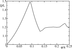
Figure 1: Dependence of the largest quantum/local value on measurement angle $\varphi$ for a Bell inequality violated maximally by the W state.

III SWAP method and results

Here we just give the basic idea of the SWAP method and in the further subsections we then give the results for self-testing of different multipartite states. For a detailed explanation of the method, we refer the reader to Ref. swap , which discusses thoroughly the bipartite case but the generalization to more parties is straightforward.

Suppose that we want to show that a multipartite state produced in a Bell experiment is close to a desired state, which we denote by $\bar{|\psi\rangle}$. The only information we have access to is the experimental violation $Q$ of a given Bell inequality $\cal{B}$. The SWAP method swap combines (i) the idea of swapping black boxes with trusted systems my with (ii) the semidefinite characterization of quantum correlations à la NPA npa .

(i) Let $\rho_{ABC}$ be the black-box system and let the trusted auxiliary qubits $A^{\prime},B^{\prime},C^{\prime}$ be prepared in the state $|0\rangle$. Then some local unitaries $U_{AA^{\prime}}$, $U_{BB^{\prime}}$, $U_{CC^{\prime}}$ are applied between the trusted systems and their respective boxes, which operations leave the trusted system in the state

$$\rho_{swap}={\textrm{Tr}}_{ABC}(U\rho_{ABC}\otimes|000\rangle\langle 000|_{A^{\prime}B^{\prime}C^{\prime}}U^{\dagger}),$$ (24)

where $U=U_{AA^{\prime}}\otimes U_{BB^{\prime}}\otimes U_{CC^{\prime}}$. We want to choose $U$ such that the fidelity

$$F=\langle\bar{\psi}|\rho_{swap}|\bar{\psi}\rangle$$ (25)

is as large as possible.

However, the virtual operation $U$ must be evaluated only from the mere knowledge of statistical data (e.g. from the amount of a Bell violation). At this point comes the NPA method to our help.

(ii) The crucial observation npa is that, for an arbitrary state $|\psi\rangle$ and set of operators $\{\hat{M}_{i}\}$, the matrix $\Gamma$ with entries $\Gamma_{ij}={\textrm{Tr}}(|\psi\rangle\langle\psi|\hat{M}_{i}^{\dagger}\hat{M}_{j})$ is positive semidefinite.

How does this help? For illustration, consider a three-party situation, and let $S$ be a set of products of the following operators $A_{x},B_{y},C_{z}$: $S=\{(\leavevmode\hbox{\small 1\normalsize\kern-3.30002pt1},A_{1},A_{2},A_{1}A_{2},A_{2}A_{1})\times(\leavevmode\hbox{\small 1\normalsize\kern-3.30002pt1},B_{1},B_{2},B_{1}B_{2},B_{2}B_{1})\times(\leavevmode\hbox{\small 1\normalsize\kern-3.30002pt1},C_{1},C_{2},C_{1}C_{2},C_{2}C_{1})$. This set has $N=5\times 5\times 5=125$ components which we denote by $M_{i}$, $i=1,\ldots,N$. According to the above remark, the $N$-dimensional $\Gamma$ matrix built up out of these operators must be positive semidefinite. Moreover, some of the matrix elements are equal or satisfy other constraints (for instance, all diagonal entries have to be 1). Such constraints we collectively denote by ${\textrm{Tr}}(\alpha_{i}\Gamma)=\delta_{i}$, $i=1,\ldots,K$, where $K$ is the number of constraints, and matrices $\alpha_{i}$ and scalars $\delta_{i}$ are associated with the constraints. Finally, noting that both the fidelity expression (25) and the Bell value are linear combinations of certain entries of the $\Gamma$ matrix, we obtain the following semidefinite programming (SDP) BV relaxation of the original problem:

$$f=\min{\textrm{Tr}(\tilde{F}\Gamma)}$$ (26)

$$\text{subject to}\,\Gamma \geq 0$$

$${\textrm{Tr}}(\alpha_{i}\Gamma) =\delta_{i}\quad(i=1,\ldots,K)$$

$${\textrm{Tr}}(\tilde{B}\Gamma) =Q,$$

where $\tilde{B}$ is the matrix which contains our Bell inequality in question and $\tilde{F}$ is the matrix encompassing the device-independent fidelity expression. Matrices $\alpha_{i}$ contain linear constraints. By solving this program, which can be done using standard SDP packages, we obtain a lower bound $f$ on the true fidelity of the quantum state $\rho_{swap}$ to a given reference state $|\bar{\psi}\rangle$.

Let us next summarize the computational resources used in solving the SDP problem (26) above. In all studied cases we used the MATLAB modeling language YALMIP yalmip . For the three-qubit computations, the size of the $\Gamma$ matrix is $125\times 125$ and the number of constraints is $K=8604$. In this case, we also increased the size of the $\Gamma$ matrix by including in sequence $S$ the following third-order terms $A_{1}A_{2}A_{1}$, $B_{1}B_{2}B_{1}$, $C_{1}C_{2}C_{1}$ (with $\Gamma$ matrix having dimension $6^{3}=216$, and $K=24436$). However, to our surprise we did not get any improvement over the previous results (the difference in all values were in the range of $10^{-8}$, which is roughly the precision of our SDP solver). In both cases, we used SeDuMi sedumi as a solver and solving the SDP for a single instance of Bell violation took about 1 hour and 1 day, respectively, on a standard desktop PC.

As for the four-qubit computations, the size of the $\Gamma$ matrix is $625\times 625$ and the number of constraints is $K=202186$. In this case, we had to use the SDPNAL solver sdpnal , which in spite of the large number of constraints solved the SDP problem (for one instance of Bell violation) within half an hour.

III.1 Self-testing of W state

We give below the details for the self-testing of the W state via the SWAP method using the three Bell expressions ${\cal{B}}_{1,2,3}$ in Table 1. The lower bound results for the fidelity $F$ are shown in Fig. 2. These curves can be directly used in Bell experiments to certify how close a black box state is to a three-qubit W state. Noting that by replacing the swaps in (24) by identity operators acting on trusted qubits which are initialized in some product state guarantees that a fidelity of $4/9$ can be achieved with respect to the W state (which value is independent of the Bell violation). Hence, we expect that the curves provide useful information only above this threshold (whose value of $4/9$ is designated by solid black line).

Also note that, for the SWAP method to work, the optimal measurement settings have to be the Pauli $Z$ and $X$, instead of our rotated measurements, in which case we have to rotate our W state correspondingly. Hence, the state we actually self-test is $|\tilde{W}\rangle=U\otimes U\otimes U|W\rangle$ and the corresponding measurements are $A_{1}=B_{1}=C_{1}=\hat{Z}$ and $A_{2}=B_{2}=C_{2}=\hat{X}$, where $U=\cos(\pi/4-\varphi/2)\leavevmode\hbox{\small 1\normalsize\kern-3.30002pt1}-i\sin(\pi/4-\varphi/2)\hat{Y}$. Since this kind of local isometry is part of the definition of self-testing, we can still identify this state with the W state. Similar rotation tricks have been applied to the GHZ and cluster states in the next subsections.

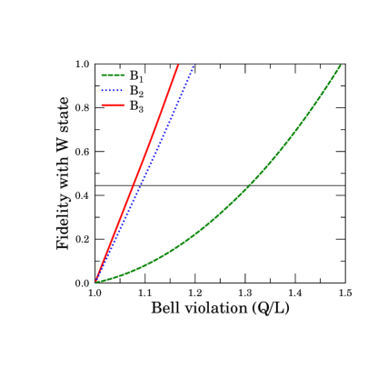
Figure 2: Robust self-testing of the W state. Minimal fidelity with respect to the ideal W state as a function of Bell violations $B_{1},B_{2}$, and $B_{3}$.

III.2 Self-testing of GHZ states

We perform robust self-testing for the (i) three-qubit GHZ state (7) using the Mermin-Bell expression (6) and for the (ii) four-qubit GHZ state (9) using the MABK-Bell expression (8). In both cases, the fidelity of $1/2$ can be attained with the $|000\rangle$ product state, hence the figure gives useful information only above this threshold value (presented with a black solid line). Please see Figure 3.

In a recent experiment, DiCarlo et al. dicarlo use superconducting circuits to implement the three-qubit GHZ state with a fidelity of $87\pm 1\%$, as assessed via full state tomography. DiCarlo et al. also evaluate the Mermin sum (6), obtaining the value $Q=3.4\pm 0.1$, or, equivalently, $Q/L=(3.4\pm 0.1)/2=1.7\pm 0.05$. For such a Bell violation, the certified fidelity value is $F=57\%$, as can be read off from solid curve 3. This nicely demonstrates the power of the device-independent approach. While our certified fidelity is (obviously) below the one reported in Ref. dicarlo , it has the advantage that it does not depend on any details of the measurement devices used in the experiment.

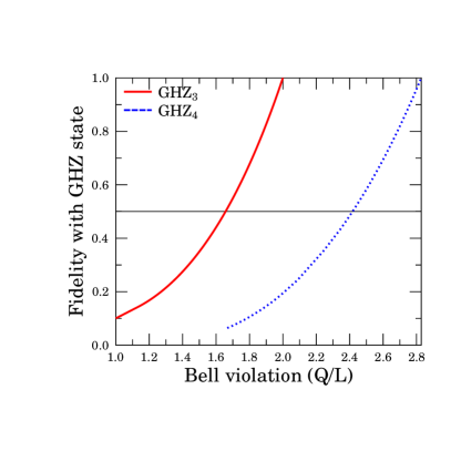
Figure 3: Robust self-testing of GHZ states. Minimal fidelity with respect to the ideal GHZ states as a function of Bell violation (Mermin and MABK inequalities).

III.3 Self-testing of the cluster state

The four-qubit linear cluster state cluster to be used in our robust self-testing is

$$|Cl\rangle=\frac{1}{2}(|0000\rangle+|0011\rangle+|1100\rangle-|1111\rangle).$$ (27)

Note that this state is not permutationally invariant.

We consider the Bell inequality that results when adding up the inequalities defined by eq. (26) and eq. (27a) in Tóth et al. clusterNL1 :

$$Toth\equiv A_{1}C_{1}D_{2}+A_{2}B_{1}C_{2}D_{2}+A_{1}C_{2}D_{1}-A_{2}B_{1}C_{1}D_{1}$$

$$+B_{2}C_{1}D_{2}+A_{2}B_{1}C_{2}D_{2}+B_{2}C_{2}D_{1}-A_{2}B_{1}C_{1}D_{1}\leq 4$$ (28)

The Tóth et al. Bell expression above can attain the algebraic maximum of 8 with a cluster state. The respective settings are $\hat{Z}$ and $\hat{X}$ up to local rotations. Hence, this inequality is a good candidate for self-testing. The minimal certified fidelity in function of the Bell violation (III.3) is shown in figure 4. We recall that the fidelity of $1/4$ can be attained with a product state, hence the figure gives useful information only above this threshold value (drawn in a black solid line).

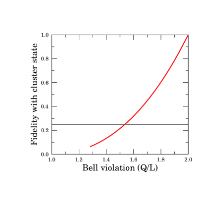
Figure 4: Robust self-testing of the cluster state. Minimal fidelity with respect to the ideal cluster state as a function of Bell violation (Tóth et al. inequality (III.3)).

The four-qubit cluster state (27) has been implemented with photons cluster_exp and recently in a system of trapped ions lanyon as well. In the first case, the two-setting Scarani et al. inequality scarani was used in a Bell experiment, for which the cluster state is not a unique eigenstate of the Bell operator giving maximal violation. Hence, it is not suitable for self-testing. In the second case, the three-setting Gühne et al.  inequality guhne was used in the Bell test, in which case the cluster state is a unique eigenstate of the Bell operator, hence suitable for self-testing. Unfortunately, the computational resources required to implement the swap method in the four-party/three-setting Bell scenario are too demanding for a normal desktop.

IV Conclusion

In this paper, we have presented an efficient algorithm based on linear programming to generate multipartite Bell inequalities which are good candidates for self-testing of permutationally invariant states. In combination with the SWAP method swap , the new inequalities and other famous Bell functionals have allowed us to self-test the W state and other notable multipartite states, such as the GHZ and cluster states. Our main findings are summarized in Figs. 2,3,4, which show how far the black-box state is (in terms of the fidelity measure) from a reference state for a given Bell violation. The presented lower bounds for the fidelity are promising from an experimental point of view, and, as we showed, some of them actually apply to recent experiments.

We have some open questions. The computational effort of the swap method for generic Bell inequalities scales badly with the number of parties. Let us recall that for four parties the number of SDP constraints are $\sim 2\times 10^{5}$. However, permutationally invariant Bell inequalities carry lots of additional symmetries over generic Bell inequalities which might be exploited to reduce the complexity of the SDP problem to be solved. This simplification may allow the swap method to be applied beyond four qubit-systems.

Self-testing of higher dimensional systems has already been demonstrated through the example of the bipartite three-outcome CGLMP inequality swap . It would be challenging to self-test three-party higher dimensional states as well, such as the fully anti-symmetric state (also called Aharonov state used in the Byzantine agreement problem aharonov ) or the generalized three-qudit GHZ state $|\psi\rangle=\sum_{i=0}^{d-1}{|i\rangle|i\rangle|i\rangle}/\sqrt{d}$ for $d\geq 3$.

Four-qubit (or even more complex) entangled states are routinely generated and characterized in various types of systems, including photons yao , ions monz ; w8qubit , and superconducting qubits dicarlo . Due to the experimentally friendly nature of the device-independent approach, we find it intriguing to perform nonlocality experiments based on our Bell expressions in Table 1 and extract certified fidelity values from our respective curves in Fig. 2.

As shown in Ref. swap , the SWAP method is also useful to self-test measurement devices in the bipartite scenario. It would be interesting to generalize our results concerning self-testing of multipartite quantum states to the realm of self-testing measurements in the multipartite scenario.

Appendix A Deriving an extra condition

Here it is shown that the mean value $\langle W|\hat{\cal B}|W\rangle$ does not change in first order on small variations around the measurement angles $\varphi_{1}$ and $\varphi_{2}$. Let us take $\varphi_{1}=\varphi+\delta_{1}$ and $\varphi_{2}=\varphi-\pi/2+\delta_{2}$. Then, neglecting second order terms, from Eq. (14) it follows:

$$\hat{M}_{1} =(c-s\delta_{1})\hat{Z}+(s+c\delta_{1})\hat{X}$$

$$\hat{M}_{2} =(s+c\delta_{2})\hat{Z}-(c-s\delta_{2})\hat{X},$$ (29)

where $c\equiv\cos\varphi$ and $s\equiv\sin\varphi$. By substituting these expressions into Eq. (13) we get through straightforward calculation:

$$\hat{G}_{1}= (c-s\delta_{1})\hat{H}_{1}+(s+c\delta_{1})\hat{H}_{2}$$

$$\hat{G}_{2}= (s+c\delta_{2})\hat{H}_{1}-(c-s\delta_{2})\hat{H}_{2}$$

$$\hat{G}_{3}= (c^{2}-2sc\delta_{1})\hat{H}_{3}+[sc+(c^{2}-s^{2})\delta_{1}]\hat{H}_{4}+$$

$$(s^{2}+2sc\delta_{1})\hat{H}_{5}$$

$$\hat{G}_{4}= 2(sc-s^{2}\delta_{1}+c^{2}\delta_{2})\hat{H}_{3}+$$

$$[s^{2}-c^{2}+2sc(\delta_{1}+\delta_{2})]\hat{H}_{4}-$$

$$2(sc+c^{2}\delta_{1}-s^{2}\delta_{2})\hat{H}_{5}$$

$$\hat{G}_{5}= (s^{2}+2sc\delta_{2})\hat{H}_{3}-[sc+(c^{2}-s^{2})\delta_{2}]\hat{H}_{4}+$$

$$(c^{2}-2sc\delta_{2})\hat{H}_{5}$$

$$\hat{G}_{6}= c^{2}(c-3s\delta_{1})\hat{H}_{6}+c[sc+(c^{2}-2s^{2})\delta_{1}]\hat{H}_{7}+$$

$$s[sc+(2c^{2}-s^{2})\delta_{1}]\hat{H}_{8}+s^{2}(s+3c\delta_{1})\hat{H}_{9}$$

$$\hat{G}_{7}= 3c(sc-2s^{2}\delta_{1}+c^{2}\delta_{2})\hat{H}_{6}+$$

$$[c(2s^{2}-c^{2})+3sc^{2}\delta_{2}+2s(2c^{2}-s^{2})\delta_{1}]\hat{H}_{7}+$$

$$[s(s^{2}-2c^{2})+3s^{2}c\delta_{2}+2c(2s^{2}-c^{2})\delta_{1}]\hat{H}_{8}-$$

$$3s(sc+2c^{2}\delta_{1}-s^{2}\delta_{2})\hat{H}_{9}$$

$$\hat{G}_{8}= 3s(sc-s^{2}\delta_{1}+2c^{2}\delta_{2})\hat{H}_{6}+$$

$$[s(s^{2}-2c^{2})+3s^{2}c\delta_{1}+2c(2s^{2}-c^{2})\delta_{2}]\hat{H}_{7}+$$

$$[c(c^{2}-2s^{2})-3sc^{2}\delta_{1}+2s(s^{2}-2c^{2})\delta_{2}]\hat{H}_{8}+$$

$$3c(sc+c^{2}\delta_{1}-2s^{2}\delta_{2})\hat{H}_{9}$$

$$\hat{G}_{9}= s^{2}(s+3c\delta_{2})\hat{H}_{6}-s[sc+(2c^{2}-s^{2})\delta_{2}]\hat{H}_{7}+$$

$$c[sc+(c^{2}-2s^{2})\delta_{2}]\hat{H}_{8}-c^{2}(c-3s\delta_{2})\hat{H}_{9}.$$ (30)

By substituting these expressions into Eq. (12) and comparing the result to Eq. (15) one can express the $\eta_{i}$ coefficients with $b_{i}$, and the angles characterizing the measurement operators. Then by using Eq. (15) one gets for the expectation value of the Bell-operator:

$$\langle W|\hat{\cal B}|W\rangle=\{(c-s\delta_{1})b_{1}+(s+c\delta_{2})b_{2}\}-$$

$$\{(c^{2}-2sc\delta_{1})b_{3}+2(sc-s^{2}\delta_{1}+c^{2}\delta_{2})b_{4}+$$

$$\vphantom{W}(s^{2}+2sc\delta_{2})b_{5}\}+$$

$$2\{(s^{2}+2sc\delta_{1})b_{3}-2(sc+c^{2}\delta_{1}-s^{2}\delta_{2})b_{4}+$$

$$\vphantom{W}(c^{2}-2sc\delta_{2})b_{5}\}-$$

$$\{c^{2}(c-3s\delta_{1})b_{6}+3c(sc-2s^{2}\delta_{1}+c^{2}\delta_{2})b_{7}+$$

$$\vphantom{W}3s(sc-s^{2}\delta_{1}+2c^{2}\delta_{2})b_{8}+s^{2}(s+3c\delta_{2})b_{9}\}+$$

$$2\{s[sc+(2c^{2}-s^{2})\delta_{1}]b_{6}+$$

$$\vphantom{W}[s(s^{2}-2c^{2})+3s^{2}c\delta_{2}+2c(2s^{2}-c^{2})\delta_{1}]b_{7}+$$

$$\vphantom{W}[c(c^{2}-2s^{2})-3sc^{2}\delta_{1}+2s(s^{2}-2c^{2})\delta_{2}]b_{8}+$$

$$\vphantom{W}c[sc+(c^{2}-2s^{2})\delta_{2}]b_{9}\}.$$ (31)

We must choose the coefficients such that the derivatives of the expression above in terms of $\delta_{1}$ and $\delta_{2}$ are zero, that is:

$$-sb_{1}+6scb_{3}+2(s^{2}-2c^{2})b_{4}+s(7c^{2}-2s^{2})b_{6}+$$

$$\vphantom{-}2c(7s^{2}-2c^{2})b_{7}+3s(s^{2}-2c^{2})b_{8}=0$$ (32)

$$-cb_{2}-6scb_{5}+2(2s^{2}-c^{2})b_{4}+c(2c^{2}-7s^{2})b_{9}+$$

$$\vphantom{-}2s(2s^{2}-7c^{2})b_{8}+3c(2s^{2}-c^{2})b_{7}=0.$$ (33)

These are necessary conditions for $\varphi$ and $\varphi-\pi/2$ to be the optimal measurement angles. They can also be expressed with the $\eta_{i}$ coefficients with this choice of angles. We can get those by substituting Eqs. (30) at $\delta_{1}=\delta_{2}=0$ into Eq. (12) and comparing the result to Eq. (15):

$$\eta_{1}= cb_{1}+sb_{2}$$

$$\eta_{2}= sb_{1}-cb_{2}$$

$$\eta_{3}= c^{2}b_{3}+2scb_{4}+s^{2}b_{5}$$

$$\eta_{4}= scb_{3}-(c^{2}-s^{2})b_{4}-scb_{5}$$

$$\eta_{5}= s^{2}b_{3}-2scb_{4}+c^{2}b_{5}$$

$$\eta_{6}= c^{3}b_{6}+3sc^{2}b_{7}+3s^{2}cb_{8}+s^{3}b_{9}$$

$$\eta_{7}= sc^{2}b_{6}-c(c^{2}-2s^{2})b_{7}+s(s^{2}-2c^{2})b_{8}-s^{2}cb_{9}$$

$$\eta_{8}= s^{2}cb_{6}+s(s^{2}-2c^{2})b_{7}+c(c^{2}-2s^{2})b_{8}+sc^{2}b_{9}$$

$$\eta_{9}= s^{3}b_{6}-3s^{2}cb_{7}+3sc^{2}b_{8}-c^{3}b_{9},$$ (34)

which can be written formally as $\eta_{i}=\sum_{j}{R_{ij}b_{j}}$, $i=1,\ldots,9$.

It is easy to see from Eq. (29) that if $\delta_{1}=\delta_{2}=0$, the $(\hat{M}_{1},\hat{M}_{2})$ pair may be expressed with $(\hat{Z},\hat{X})$ the same way than the other way around. Therefore, Eqs. (34) and the inverse relationships has the same coefficients, i.e. $b_{i}=\sum_{j}{R_{ij}\eta_{j}}$, $i=1,\ldots,9$.

Now let us add Eq. (32) to Eq. (33). Comparing the result to Eqs. (34) it is fairly easy to see that the result is:

$$-\eta_{2}+6\eta_{4}+7\eta_{7}-2\eta_{9}=0.$$ (35)

However, if the $|W\rangle$ is an eigenstate of the Bell-operator, this relationship is automatically fulfilled as the equation follows from Eqs. (19). If we multiply Eq. (32) by $c^{2}$ and Eq. (33) by $s^{2}$, subtract them from each other, and use $c^{2}+s^{2}=1$ several times, a somewhat lengthier calculation does lead to an independent, fairly simple equation:

$$sc(-\eta_{1}+2\eta_{3}+4\eta_{5}+3\eta_{6}+2\eta_{8})+4(c^{2}-s^{2})(\eta_{4}+\eta_{7})=0.$$ (36)

This is the condition appearing in Eq. (21) in the main text. We note that the derivation of Eq. (36) and the spurious Eq. (35) is not a crucial step. Instead of Eq. (21), we could have taken both Eqs. (32,33) directly as constraints for the linear program.

References

- (1) R. Horodecki, P. Horodecki, M. Horodecki, and K. Horodecki, Rev. Mod. Phys. 81, 865 (2009).
- (2) O. Gühne and G. Tóth, Phys. Rep. 474, 1 (2009).
- (3) D. Rosset, R. Ferretti-Schöbitz, J-D. Bancal, N. Gisin, and Y-C. Liang, Phys. Rev. A 86, 062325 (2012).
- (4) G. Tóth et al., Phys. Rev. Lett. 105, 250403 (2010); W. Wieczorek et al., Phys. Rev. Lett. 103, 020504 (2009).
- (5) C. Schwemmer, G. Tóth, A. Niggebaum, T. Moroder, D. Gross, O. Gühne, H. Weinfurter, arXiv:1401.7526 (2014).
- (6) T. Monz et al., Phys. Rev. Lett. 106, 130506 (2011).
- (7) B.P. Lanyon, M. Zwerger, P. Jurcevic, C. Hempel, W. Dür, H.J. Briegel, R. Blatt, and C.F. Roos, Phys. Rev. Lett. 112, 100403 (2014).
- (8) D. Gross, Y.-K. Liu, S. T. Flammia, S. Becker, and J. Eisert, Phys. Rev. Lett. 105, 150401 (2010).
- (9) M. Cramer, M. B. Plenio, S. T. Flammia, R. Somma, D. Gross, S. D. Bartlett, O. Landon-Cardinal, D. Poulin, and Y.-K. Liu, Nat. Commun. 1, 149 (2010).
- (10) V. Scarani, arXiv:1303.3081 (2013).
- (11) D. Mayers and A. Yao, Quant. Inf. Comput. 4, 273 (2004).
- (12) S.J. Summers, R.F. Werner, Commun. Math. Phys. 110, 247 (1987); S. Popescu, D. Rohrlich, Phys. Lett. A 169, 411 (1992); B.S. Tsirelson, Hadronic Journal Supplement 8, 329 (1993).
- (13) C.-E. Bardyn, T.C.H. Liew, S. Massar, M. McKague, and V. Scarani, Phys. Rev. A 80, 062327 (2009); M. McKague, T.H. Yang, and V. Scarani, J. Phys. A: Math. Theor. 45, 455304 (2012); C.A. Miller and Y. Shi, arXiv:1207.1819 (2012); B.W. Reichardt, F. Unger and U. Vazirani, Nature 496, 456 (2013); T.H. Yang and M. Navascués, Phys. Rev. A 8, 050102(R) (2013).
- (14) T.H. Yang, T. Vertesi, J.-D. Bancal, V. Scarani, and M. Navascues, arXiv:1307.7053 (2013); arXiv:1406.7127 (2014).
- (15) J.F. Clauser, M.A. Horne, A. Shimony, and R.A. Holt, Phys. Rev. Lett. 23, 880 (1969).
- (16) W. Dur, G. Vidal, and J.I. Cirac, Phys. Rev. A 62, 062314 (2000).
- (17) D.M. Greenberger, M.A. Horne, A. Zeilinger, Bells Theorem, Quantum Theory, and Conceptions of the Universe (ed. M. Kafatos, Kluwer Academic, Dordrecht, Holland, 1989), p. 69.
- (18) H.J. Briegel and R. Raussendorf, Phys. Rev. Lett. 86, 910 (2001); R. Raussendorf, H. J. Briegel, Phys. Rev. Lett. 86, 5188 (2001).
- (19) M. Eibl, S. Gaertner, M. Bourennane, C. Kurtsiefer, M. Zukowski, and H. Weinfurter, Phys. Rev. Lett. 90, 200403 (2003).
- (20) J.-W. Pan, D. Bouwmeester, M. Daniell, H. Weinfurter, and A. Zeilinger, Nature 403, 515 (2000); M. Eibl, N. Kiesel, M. Bourennane, C. Kurtsiefer, and H. Weinfurter, Phys. Rev. Lett. 92, 077901 (2004); Z. Zhao, T. Yang, Y.-A. Chen, A.-N. Zhang, M. Zukowski, and J.-W. Pan, Phys. Rev. Lett. 91, 180401 (2003).
- (21) P. Walther, M. Aspelmeyer, K. J. Resch, and A. Zeilinger, Phys. Rev. Lett. 95, 020403 (2005); N. Kiesel et al., Phys. Rev. Lett. 95, 210502 (2005).
- (22) N. D. Mermin, Am. J. Phys. 58, 731 (1990).
- (23) M. McKague, arXiv:1010.1989 (2010).
- (24) J.-D. Bancal, N. Gisin, Y.-C. Liang, and S. Pironio, Phys. Rev. Lett. 106, 250404 (2011); K. F. Pal, T. Vertesi, Phys. Rev. A 83, 062123 (2011).
- (25) J. T. Barreiro, J-D. Bancal, P. Schindler, D. Nigg, M. Hennrich, T. Monz, N. Gisin, and R. Blatt, Nature Physics 9, 559 (2013).
- (26) T. Moroder, J.-D. Bancal, Y.-C. Liang, M. Hofmann and O. Gühne, Phys. Rev. Lett. 111, 030501 (2013).
- (27) G. Vidal and R. F. Werner, Phys. Rev. A 65, 032314 (2002).
- (28) N. Brunner, J. Sharam, and T. Vértesi, Phys. Rev. Lett. 108, 110501 (2012).
- (29) X. Wu, Y. Cai, T. H. Yang, H. N. Le, J.-D. Bancal and V. Scarani, arXiv:1407.5769.
- (30) J. S. Bell, Physics 1, 195 (1964); N. Brunner, D. Cavalcanti, S. Pironio, V. Scarani and S. Wehner, Rev. Mod. Phys. 86, 419 (2014).
- (31) N. D. Mermin, Phys. Rev. Lett. 65, 1838 (1990).
- (32) M. Ardehali, Phys. Rev. A 46, 5375 (1992); A.V. Belinskii and D.N. Klyshko, Phys. Usp. 36, 653 (1993).
- (33) J.-D. Bancal, N. Gisin, and S. Pironio, J. Phys. A: Math. Theor. 43, 385303 (2010); N. Brunner, J. Sharam, and T. Vertesi, Phys. Rev. Lett. 108, 110501 (2012); J. Tura, A. B. Sainz, T. Vertesi, A. Acin, M. Lewenstein, and R. Augusiak, arXiv:1312.0265 (2013).
- (34) R.H. Dicke, Phys. Rev. 93, 99 (1954).
- (35) R.F. Werner and M.M. Wolf, Quantum Inf. Comput. 1, 1 (2001); K.F. Pál and T. Vértesi, Phys. Rev. A 82, 022116 (2010).
- (36) Ll. Masanes, arXiv:quant-ph/0512100 (2005).
- (37) M. Navascués, S. Pironio, and A. Acín, Phys. Rev. Lett. 98, 010401 (2007); M. Navascués, S. Pironio and A. Acín, New J. Phys. 10, 073013 (2008).
- (38) S.P. Boyd and L. Vandenberghe, Convex Optimization, Cambridge University Press, 2004.
- (39) J. Löfberg, YALMIP: A Toolbox for Modeling and Optimization in MATLAB, Proceedings of the CACSD Conference (Taipei, Taiwan, 2004).
- (40) J.F. Sturm, Using SeDuMi 1.02, a MATLAB toolbox for optimization over symmetric cones, Optimization Methods and Software 11 625 (1999).
- (41) X. Zhao, D. Sun, and K.-C. Toh, SIAM J. Optim. 20, 1737 (2010).
- (42) L. DiCarlo et al., Nature 467, 574 (2010).
- (43) G. Toth, O. Guehne, H. J. Briegel, Phs. Rev. A 73, 022303 (2006).
- (44) V. Scarani, A. Acín, E. Schenck, and M. Aspelmeyer, Phys. Rev. A 71, 042325 (2005).
- (45) O. Gühne, G. Tóth, P. Hyllus, and H.J. Briegel, Phys. Rev. Lett. 95, 120405 (2005).
- (46) M. Fitzi, N. Gisin, U. Maurer, Phys. Rev. Lett. 87, 217901 (2001).
- (47) X.-C. Yao et al., Nat. Phot. 6, 225 (2012).
- (48) H. Häffner, W. Hänsel, C. Roos, J. Benhelm, et al., Nature 438, 643 (2005).