Reference analysis of the signal + background model in counting experiments II. Approximate reference prior

Abstract

The objective Bayesian treatment of a model representing two independent Poisson processes, labelled as “signal” and “background” and both contributing additively to the total number of counted events, is considered. It is shown that the reference prior for the parameter of interest (the signal intensity) can be well approximated by the widely (ab)used flat prior only when the expected background is very high. On the other hand, a very simple approximation (the limiting form of the reference prior for perfect prior background knowledge) can be safely used over a large portion of the background parameters space. The resulting approximate reference posterior is a Gamma density whose parameters are related to the observed counts. This limiting form is simpler than the result obtained with a flat prior, with the additional advantage of representing a much closer approximation to the reference posterior in all cases. Hence such limiting prior should be considered a better default or conventional prior than the uniform prior. On the computing side, it is shown that a 2-parameter fitting function is able to reproduce extremely well the reference prior for any background prior. Thus, it can be useful in applications requiring the evaluation of the reference prior for a very large number of times.
The published version JINST 9 (2014) T10006 (10.1088/1748-0221/9/10/T10006) has a typo in the normalization constant $N$ of eq. (12), fixed here.

1 Introduction

This document complements and extends the results shown in Ref. [1] (hereafter Paper I), in which the reference analysis is performed of the signal + background model in counting experiments, when partial information is available about the background and an objective Bayesian solution is desired. In the model, signal and background events come from two independent Poisson sources, so that the total number $n\geq 0$ of observed counts is distributed accordingly to

$$\text{Poi}(n|s+b)=\frac{(s+b)^{n}}{n!}\,e^{-(s+b)}$$ (1)

The goal is to perform statistical inference on the signal strength $s\geq 0$, hence the background strength $b\geq 0$ is a nuisance parameter. The starting point is the Bayes’ theorem

$$p(s,b|n)\propto\text{Poi}(n|s+b)\,p(s)\,p(b)$$ (2)

which gives the joint posterior probability density $p(s,b|n)$ of signal and background strengths, given the observed number $n$ of events. The joint posterior is proportional to the product of the likelihood function — that is (1) when considered as a function of $s$ and $b$ for fixed $n$ — with the prior densities $p(s)\,p(b)$ of signal and background. After integrating over $b$, one gets the marginal posterior density $p(s|n)$ which represents the full solution of the inference problem. From $p(s|n)$ one can compute summary information like e.g. the posterior expectation or most probable value, enclosed by intervals representing some given probability, say 68.3% or 95% posterior probability.

In Paper I the very common situation is considered in which one claims no prior information on the signal $s$, but does have prior estimates of the background expectation $E[b]$ and standard deviation $\sqrt{V[b]}$ (the square root of the prior variance). These two values are sufficient to specify uniquely the prior density, if the latter is chosen to be a Gamma density

$$p(b)=\text{Ga}(b|\alpha,\beta)=\frac{\beta^{\alpha}}{\Gamma(\alpha)}\,b^{\alpha-1}\,e^{-\beta b}$$ (3)

(the conjugate prior of the Poisson model) with shape parameter $\alpha>0$ and rate parameter $\beta>0$ fixed by requiring $E[b]=\alpha/\beta$ and $V[b]=\alpha/\beta^{2}$.

The same Poisson model (1), when assuming no prior knowledge about both the signal and the background, has been addressed by [2] and [3], where a reference prior is found for both signal and background. However in practical applications, expecially when a search for rare or new phenomena is performed, the background is known quite well (the discovery of the Higgs boson is one example [4, 5]). Hence we restrict ourselves to the inference problems about the signal strength $s$, when there is at least some knowledge of the background yield summarized by the prior background expectation $E[b]$ and variance $V[b]$ (or standard deviation).

Paper I finds the reference prior for the signal starting from the marginal model

$$P(n|s)=\int_{0}^{\infty}\text{Poi}(n|s+b)\,\text{Ga}(b|\alpha,\beta)\,\text{d}b$$ (4)

and following the algorithm explained in [6], which requires the computation of the Fisher’s information function

$$I(s)=-E\left[\left(\frac{\partial^{2}}{\partial s^{2}}\log p(k|s)\right)\right]$$ (5)

As the resulting reference prior $\pi(s)\propto|I(s)|^{1/2}$ is not integrable over the positive real line, it has an arbitrary scale factor. It should be emphasized that, provided that the corresponding posterior is a proper density, this is not a problem for the reference prior, which is formally constructed in such a way to maximize the amount of missing prior information and does not represent one’s degree of belief [7, 8, 9]. The choice made in Paper I is to define

$$\pi(s)=\frac{|I(s)|^{1/2}}{|I(0)|^{1/2}}$$ (6)

which makes it trivial to compare it against the uniform prior, so widespread that it can be considered a conventional prior.

As noted in Paper I (and references therein), the flat prior is often presented as “noninformative”, which is not the case, as for the current problem it is not the result of a formal procedure to construct an objective prior. At the same time, it can not be an informative prior, because it is not normalizable (hence can not represent a degree of belief): strictly speaking it has no formal justification. In facts, the (ab)use of the uniform prior is the most important source of criticism toward the Bayesian approach in scientific inference. Nevertheless, the flat prior may provide a good approximation to the reference prior in some case, although this is not a general rule.

The function (6) is monotonically decreasing and depends on the shape and rate parameters describing the prior of the background. It is flatter for increasing background expectation $E[b]=\alpha/\beta$ and for decreasing prior background relative uncertainty $\sigma[b]/E[b]=1/\sqrt{\alpha}$. Thus for increasing $\alpha$ and decreasing $\beta$, the flat prior may provide a good approximation to an objective prior, although it is the user’s responsibility to decide when the difference with respect to $\pi(s)$ is acceptably small.

The reference prior $\pi(s)$ obtained in Paper I has the form of an infinite series, as shown in the next section. Although its implementation in a computer program has good performance when following the recommendations of Appendix A of Paper I, some users consider it too complicated and error-prone to write the corresponding code. For this reason, they end up into using the flat prior as the “conventional” choice, despite from the known issues of this prior (it is mathematically ill-defined and many people do not consider it “objective”, as it gives absurdly high weights to large values of the signal, which are known not to be true). Hence it is important to find the cases in which the use of $\pi(s)$ is not required.

Luckily enough, a very simple expression exists for the limiting case of perfect background knowledge, which provides a good approximation in many practical problems and is closer to the reference prior than the flat prior. The corresponding posterior is a Gamma function which approximates the reference posterior much better than the posterior obtained with a flat prior (the marginal model given by eq. (4) below). This solution is so simple that there is really no motivation to adopt a flat prior. Below, we will see how well this approximation works. Even when it is not a perfect approximation, it is usually closer to the full reference prior than the constant prior. For this reason, it is recommended as the default or conventional prior whenever the use of the full reference prior is considered too complicated.

In practical applications, the performance can be improved if the reference prior is evaluated only at few tens of points and interpolated with a fitting function to be used in the following computations, as a probability density function may need to be evaluated a very large number of times. The limiting properties of the reference prior suggest the form of a 1-parameter fitting function which is easy to program and provides a good approximation to the reference prior over a wide portion of the parameters space. Furthermore, a 2-parameter approximate reference prior, available in closed form and very quick to compute, is practically equivalent to $\pi(s)$ for the entire parameters range scanned in this work. This fitting function can be used to speed-up the computation of the reference prior with no precision losses. Thus it is has been exploited in the Bayesian Analysis Toolkit [10], which is the first publicly available implementation of the reference prior $\pi(s)$ known to the author. Appendix A shows an example of C++ code to be used with BAT. For the users who do not rely on BAT, a table of values of $\pi(s)$ for $s\in[0,70]$ for all background parameters examined in section 3 is freely available on Zenodo (10.5281/zenodo.11896), to obtain quick approximations as described below and in Appendix C.

2 The reference prior and posterior densities

Although the marginal model (4) does not depend explicitly on the background, it still depends on the background shape $\alpha$ and rate $\beta$ parameters via the integration. Paper I shows that the marginal model can be written as

$$P(n|s)=\left(\frac{\beta}{1+\beta}\right)^{\!\alpha}e^{-s}\,f(s;n,\alpha,\beta)$$ (7)

where the polynomial

$$f(s;n,\alpha,\beta)=\sum_{m=0}^{n}\binom{\alpha+m-1}{m}\frac{s^{n-m}}{(n-m)!\,(1+\beta)^{m}}$$ (8)

behaves like $(s+\alpha/\beta)^{n}$ when both $\alpha,\beta$ are very large.

Hence the reference prior also depends on the background parameters, and it does so via the Fisher’s information function

$$|I(s)|^{1/2}=\left|\left(\frac{\beta}{1+\beta}\right)^{\!\alpha}e^{-s}\,\sum_{n=0}^{\infty}\frac{[f(s;n,\alpha,\beta)]^{2}}{f(s;n+1,\alpha,\beta)}-1\right|^{1/2}$$ (9)

which involves an infinite sum over terms featuring the polynomial (8). This function is not integrable, hence one is free to choose a multiplicative constant. We define the reference prior as in eq. (6), which is the recommended expression in practical computations.

The marginal reference posterior for the signal yield $s$ is

$$p(s|n)\propto\left(\frac{\beta}{1+\beta}\right)^{\!\alpha}e^{-s}\,f(s;n,\alpha,\beta)\,\pi(s)$$ (10)

which is always a proper density, hence the normalization constant is just the integral of the expression above.

In Paper I it was shown that, in the limiting case of perfect prior information about the background, the reference prior becomes proportional to $(s+b_{0})^{-1/2}$. This is the Jeffreys’ prior for the variable $s^{\prime}\equiv s+b_{0}$, a quite natural result. More precisely, the limiting prior which matches the convention that $\pi(0)=1$ is

$$\pi_{0}(s)\equiv\sqrt{\frac{b_{0}}{s+b_{0}}}$$ (11)

when one has perfect prior knowledge of the background. It is then interesting to check that the posterior also matches the result obtained with Jeffreys’ prior, which for $n$ observed counts is $p(s^{\prime}|n)=\text{Ga}(s^{\prime}|n+\frac{1}{2},1)$.

By substituting $\alpha=b_{0}\beta$ in (8) and taking the limit $\beta\to\infty$ while keeping $\beta=\alpha/b_{0}$ constant, such that the background prior (3) tends to $\delta(b-b_{0})$, one gets

$$\begin{split}f(s;n+1,\alpha,\beta)&\xrightarrow[\beta=\alpha/b_{0}]{\alpha\to\infty}\frac{s^{n}}{n!}+\frac{s^{n-1}\,b_{0}}{(n-1)!}+\frac{s^{n-2}\,b_{0}^{2}}{2(n-2)!}+\frac{s^{n-3}\,b_{0}^{3}}{3!(n-3)!}+\cdots+\frac{b_{0}^{n}}{n!}\\ &=\sum_{k=0}^{n}\binom{n}{k}\,s^{n-k}\,b_{0}^{k}=(s+b_{0})^{n}\end{split}$$

In the same limit, $[\beta/(1+\beta)]^{\alpha}\to e^{-b_{0}}$ and eq. (10) gives $p_{0}(s|n)\propto e^{-(s+b_{0})}\,(s+b_{0})^{n-1/2}$ i.e. the kernel of the Gamma density $\text{Ga}(s+b_{0}|n+\tfrac{1}{2},1)$, as expected. In conclusion, the properly normalized limiting reference posterior is

$$p_{0}(s|n)=\frac{1}{N}\text{Ga}(s+\tfrac{\alpha}{\beta}|n+\tfrac{1}{2},1)$$ (12)

where the normalization constant is

$$N=\int_{0}^{\infty}\text{Ga}(s+\tfrac{\alpha}{\beta}|n+\tfrac{1}{2},1)\,\text{d}s=\int_{\alpha/\beta}^{\infty}\text{Ga}(x|n+\frac{1}{2},1)\,\text{d}x$$

Compared to the posterior obtained with a flat prior, proportional to the marginal model (7) (see also Appendix B), the limiting reference posterior is simpler and easier to implement (most data analysis packages include the Gamma function, so no coding is needed). Hence it is a much more appealing conventional solution, provided that it behaves not much worse than the flat prior. Actually it comes out that the limiting reference posterior (12) is a much better approximation to the reference posterior than (7), so that there is really no reason to continue using the flat prior.

In the following section, we will investigate the performance of the approximate reference prior obtained by setting $b_{0}=E[b]$ in eq. (11). This is equivalent to ignoring the uncertainty on the background in the signal region. Hence we expect it to work well whenever the relative uncertainty $\sqrt{V[b]}/E[b]=1/\sqrt{\alpha}$ is small, that is for large values of the shape parameter. The good surprise is that, even when the relative uncertainty is sizable, $\pi_{0}(s)$ is very often a much better approximation to the reference prior than a flat prior.

3 Properties of the limiting reference prior

In order to see how well the limiting reference prior $\pi_{0}(s)=\sqrt{E[b]/(s+E[b])}$ approximates the reference prior $\pi(s)$, the function $\pi_{0}(s)$ has been computed over many points in the $(\alpha,\beta)$ parameter space. A uniform logarithmic scan was performed, with a factor of 2 spanned by each parameter every 5 steps. Figure 1 shows the points of the parameters space $(\alpha,\beta)$ which have been used in this paper, together with the corresponding values of the expected background $E[b]=\alpha/\beta$ and relative uncertainty $\sigma[b]/E[b]=1/\sqrt{\alpha}$.

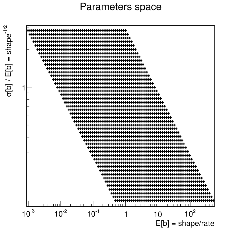
Figure 1: Scan of the background prior parameters space (left) and corresponding prior expectation and relative uncertainty (right).

The most useful comparison is among the posteriors obtained with different priors, and is definitely a very good check for any particular problem under analysis. However, the posterior is conditional on the number $n$ of observed counts, which can range from zero to infinity, hence one would need to consider a very large number of possible combinations, which is unfeasible. Figure 2 provides just one example, showing the ratio between the posterior expected signal computed with the flat or limiting prior and the reference posterior mean, when $n=1$ (very far from the asymptotic regime, in which we know that the posteriors will be practically the same). The flat prior always overestimates the posterior mean, approaching the reference posterior expectation when the background expectation is higher (i.e. toward the top-left region in the parameters space). This is the obvious consequence of assigning a costant weight to all possible values of the signal (in contrast, the reference prior assigns a monotonically decreasing weight to larger signal intensities). On the other hand, the limiting reference prior expectation approaches the reference posterior mean from below, being closer than the result obtained with a flat prior over a large portion of the parameters space. As an example, the regions in which the agreement is not worse than 5% are also shown in the figure.

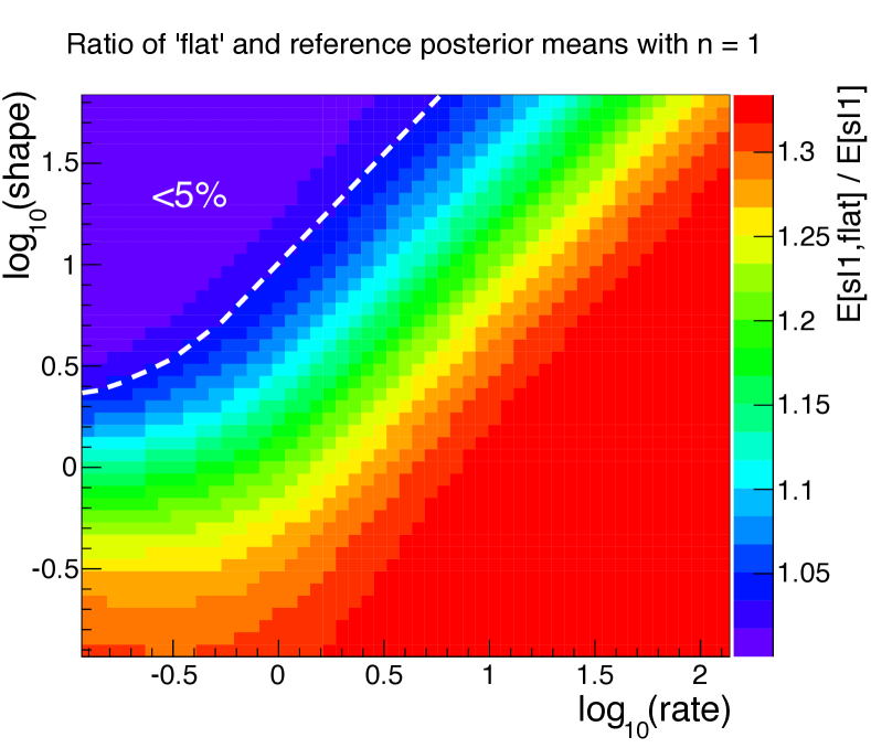
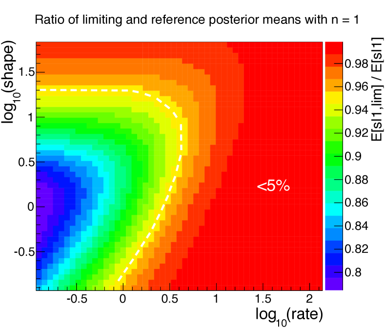
Figure 2: Ratio of posterior means for $n=1$ observed counts. Left: the posterior corresponding to the flat prior $p(s)=1$ is compared to the reference posterior $p(s|n=1)$. Right: the limiting reference posterior obtained when using the limiting prior $\pi_{0}(s)$ is compared to the reference posterior.

As it is impractical to compare the posteriors for various values of $n$, we focus in the following on the differences between priors. There are several ways of quantifying the “distance” between two probability distributions. Among the most common ones, we have

$$d_{a}=\left(\int|p(x)-q(x)|^{a}\,\text{d}x\right)^{\!1/a}$$ (13)

where $a=1$ corresponds to the area bracketed by the two densities $p(x)$ and $q(x)$, $a=2$ is the usual RMS difference, and $a\to\infty$ gives $d_{\infty}=\max|p(x)-q(x)|$, the maximum of the point-wise comparison.

All of them are defined for proper densities, whereas in our case we have improper priors to be compared. Here we avoid problems related to the integration over an unlimited domain by restricting it to a reasonably wide range, chosen to be $[0,70]$. In addition, we choose the RMS distance $d_{2}$ and normalize the difference by dividing by the integral of the reference prior over the same interval. Figure 3 shows the expected background and the relative RMS difference between $\pi_{0}(s)$ and $\pi(s)$, as a function of $\alpha$ and $\beta$.

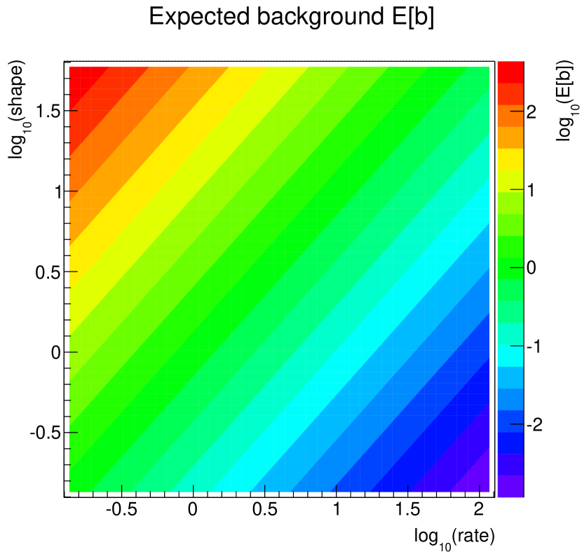
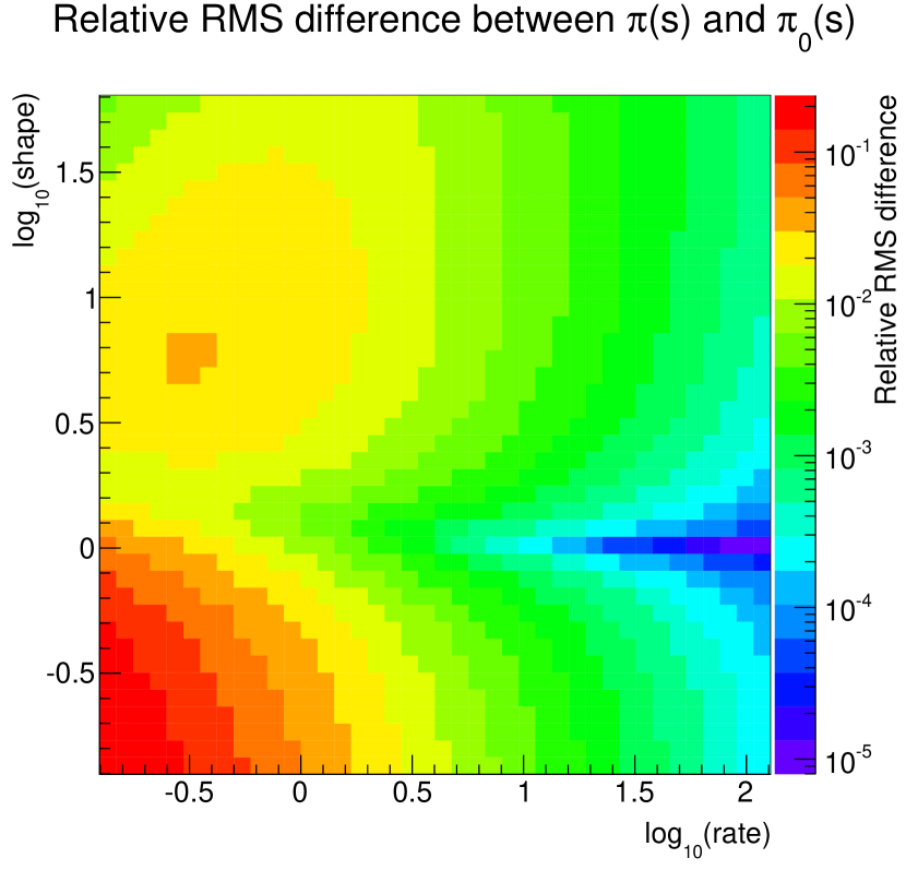
Figure 3: Expected background (left) and relative RMS difference between $\pi(s)$ and $\pi_{0}(s)$ (right).

In practice, the use of the reference prior is recommended mostly when the signal is small or absent: what really matters is the difference between the posteriors, and this becames negligible very quickly for increasing number $n$ of observed counts. The dependence on the choice of the prior is strongest when $n$ is very small or zero, which implies that the sum of signal and background is very small. In addition, here we are comparing monotonically decreasing functions all starting from the same positive value (one at the origin) and all asymptotically reaching zero: their relative difference (apart from the maximum point-wise separation) becomes smaller and smaller for increasing values of the argument. This means that, although somewhat arbitrary, the choice of looking at the relative RMS difference over $[0,70]$ is sufficient to capture all relevant aspects of the comparison and can serve as a useful guideline for deciding when one should use the full reference prior or can safely use the approximate expression.

For most practical purposes, a relative RMS difference below 1% is acceptable, as this is the order of magnitude of the maximum change in the posterior in the limit of very few or zero observed counts. Hence we will assume that a disagreement not larger than 1% is tolerable in this paper. On the other hand, it should be emphasized that a threshold at 1% is quite conservative. In most applications larger deviations can be tolerated, as the posteriors will quickly become indistinguishable for increasing number $n$ of observed counts. In addition, the common practice is to summarize the posterior by providing one value (e.g. the expectation) and some estimate of its uncertainty (e.g. the shortest interval covering 68.3% posterior probability), by rounding the values to the minimum meaningful number of digits. Often, this summary is quite robust compared to relative RMS differences of several percent. Nevertheless, the notion of “acceptable difference” is application dependent, and the researcher should state which is the criterion dictating the choice of the prior.

The right panel of figure 3 shows that the limiting reference prior is satisfactory (differing by less than 1%) when the rate parameter is larger than 4, and in some case even for lower values (depending on the shape parameter).

4 Computing the reference prior

The reference prior (6) can be evaluated iteratively, by computing the next element of its infinite series until the difference with respect to the previous result becomes smaller than a predefined tolerance. When $s$ is large, more terms need to be computed to achieve a predefined precision, which means that the calculation become slower. In addition, the CPU time may depend on the background parameters. For example the author’s private C++ code works with a tolerance of $10^{-6}$, a bit larger than the accuracy of single-precision floating-point values. The average CPU time per evaluated point with $s\in[0,70]$ ranges from 0.5 ms to 4.5 ms on the author’s laptop, with the lowest value spanning over most of the parameters space, apart from the top-left corner (shape higher than 10, rate lower than 1; figure 4), where it increases rapidly.

With the goal of improving the performance of numerical evaluations, approximations of the reference prior were searched for, which could provide better results than the limiting reference prior (11). Closed form expressions were found, which allow to significantly reduce the computing time. The 2-parameter approximation illustrated in section 4.2 below requires 0.10–0.24  µs per call, independently of the region in the $(\alpha,\beta)$ space, providing a speed-up in the range $10^{3}$–$2\times 10^{4}$.

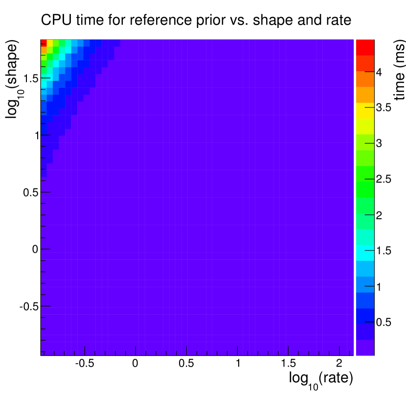
Figure 4: Average CPU time per call required by the author’s private C++ code computing the reference prior $\pi(s)$.

4.1 A 1-parameter approximation

Inspired by the limiting form (11), one may look for a simple approximation of $\pi(s)$ in which a single parameter is tuned to obtain the best agreement with the reference prior. A fit has been performed with the function

$$f(s;C)=\sqrt{\frac{C}{s+C}}$$ (14)

where $C>0$ is the single unknown parameter, over the parameters space. The value of the reference prior $\pi(s)$ has been computed at equally spaced steps in the range $s\in[0,70]$. The fit quality and best parameter values are shown in figure 5. Clearly, $C\to E[b]$ in the limit of perfect background knowledge, where $\pi_{0}(s)$ works well (figure 6, right panel).

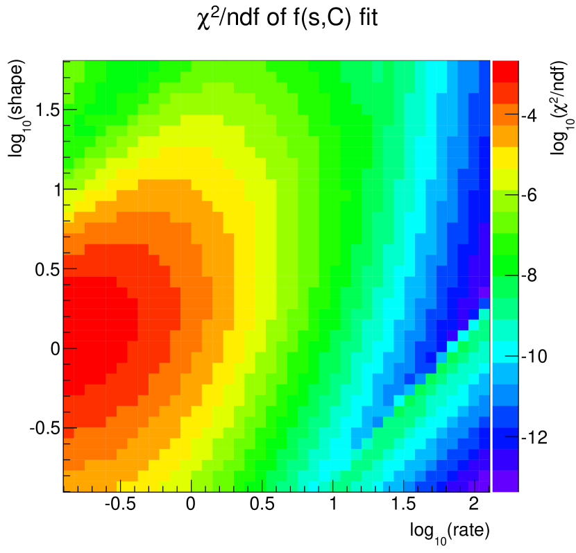
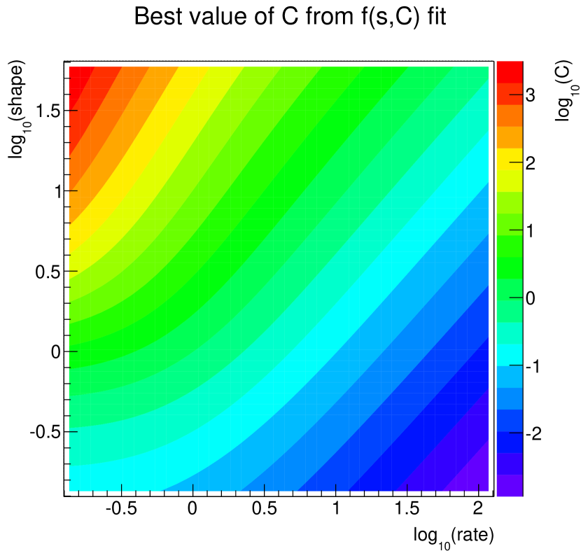
Figure 5: Fit quality (left) and best parameter value (right).

The relative RMS difference between $f(s;C)$ and $\pi(s)$ is shown in figure 6, left panel. The function (14) provides a good approximation, with a relative RMS difference below 1%, whenever both shape and rate parameters are not small (i.e. when they are at least few units). Our quality threshold is exceeded only if $\alpha<2.5$ and $\beta<0.6$.

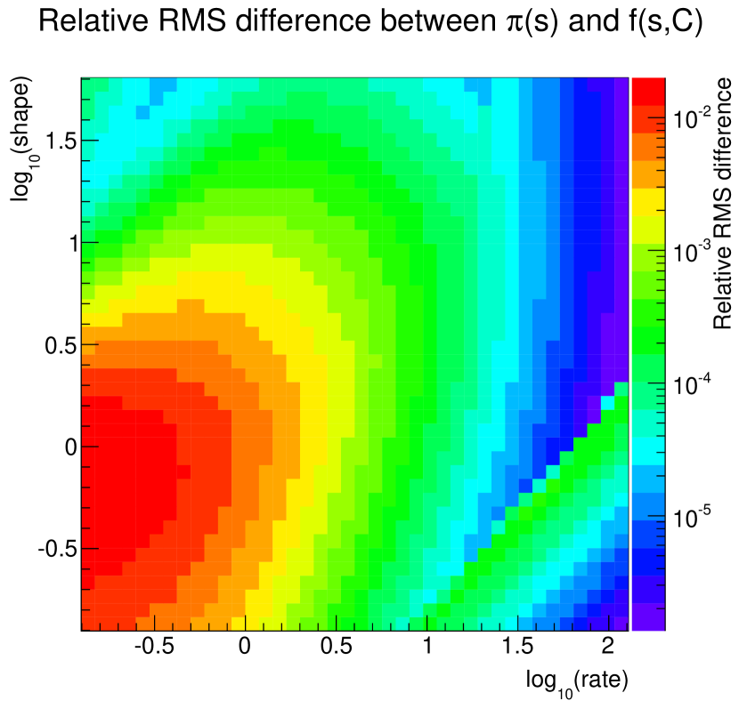
Figure 6: Relative RMS difference between the best fitting function $f(s;C)$ and the reference prior $\pi(s)$ (left), and ratio between the fit parameter and the prior background expectation (right).

When there is very good prior knowledge of the background, the limiting value for the $C$ parameter is the prior background expectation, hence it is instructive to look at the ratio $C/E[b]$ over the parameter space. As the limiting situation which we are considering involves a fixed background expectation and a decreasing relative precision $\sqrt{V[b]}/E[b]=1/\sqrt{\alpha}$, we expect that far from the conditions of perfect background knowledge the departure of $C/E[b]$ will depend on the shape parameter only. Indeed, the right plot in figure 6 shows that for small rate values, the ratio is a monotonically increasing function of the shape parameter, whereas for large values of the rate parameter (in practice, when $\beta$ is at least about ten), $C$ is practically equivalent to the prior background expectation. In particular, the logarithm of the ratio $C/E[b]$ can be well fitted by an arcotangent function of the logarithm of the shape parameter, whose amplitude (the distance between the two asymptotic values) goes to zero very quickly with increasing $\beta$ values (a Gaussian fit well reproduces the amplitude as a function of the logarithm of the rate parameter in the range studied here).

In summary, when the rate parameter is larger than several units the limiting reference prior (11) already provides a good approximation. In addition, for smaller values of $\beta$ the 1-parameter function (14) can fit the reference prior well enough, provided that the shape parameter is larger than few units. However, this approximation does not satisfy our requirement over the entire parameter space, hence we look for something better.

4.2 A 2-parameter approximation

A function which fits the reference prior better than (14) and can well reproduce $\pi(s)$ over the entire portion of parameters space considered here is

$$f(s;A,B)=\sqrt{\frac{A\exp(B\,s^{E})}{s+A\exp(B\,s^{E})}}$$ (15)

It coincides with (14) when setting the parameter $D$ to zero and should be used if $\alpha<2.5$ and $\beta<0.6$ and $n$ is small. The power $E$ of $s$ in the exponent was found not to change appreciably over the entire parameter space, and was treated as a fixed parameter with value $E=0.125$ when producing the plots shown in figures 7, 8 and 9 (only $A$ and $B$ were left free to vary in the fits). The difference with the reference prior is very small and completely negligible in any practical application.

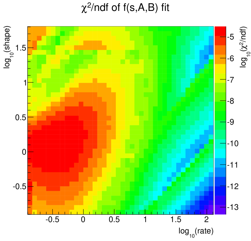
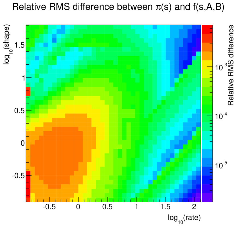
Figure 7: Fit quality (left) and relative RMS difference between the best fitting function $f(s;A,B)$ and the reference prior $\pi(s)$ (right).

Figure 7 shows the goodness of fit of (15) and the relative RMS difference between $f(s;A,B)$ and $\pi(s)$. The latter is one order of magnitude better than the result obtained with $f(s;C)$, and is always smaller that 1% over the entire portion of the parameters space investigated here. Hence the form (15) is well suited for practically all applications. Indeed, this function can be optionally used in BAT [10] to speed-up the computation of the reference prior: the latter is initially computed over a number of discrete $s$ values, then a best fit with $f(s;A,B)$ is performed, and the latter is used in all following computations (a similar approach is illustrated in Appendix C).

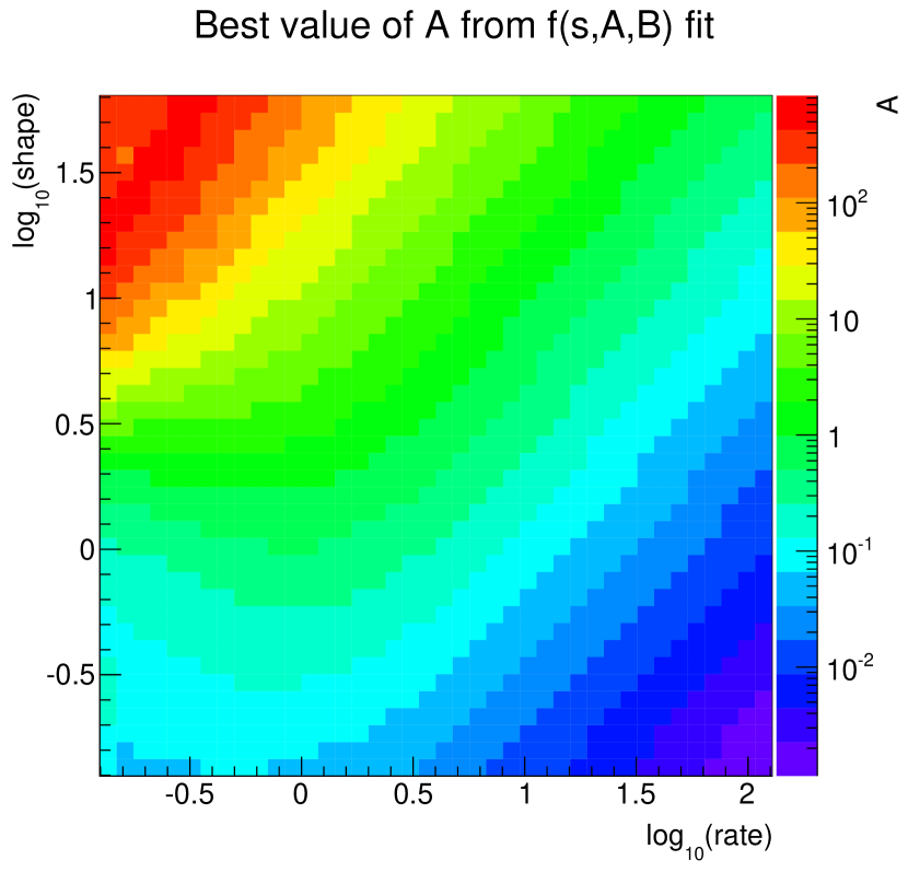
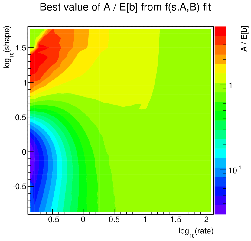
Figure 8: Value of the $A$ parameter for the best fitting function $f(s;A,B)$ (left), and its ratio with the prior background expectation (right).

As shown in figure 8, the best value of the $A$ parameter basically coincides with the best value of $C$ whenever $f(s;C)$ represents a good approximation. In this portion of the parameters space (say for $\beta$ above several units), the $B$ parameter is indeed so small that one can round it off to zero (figure 9).

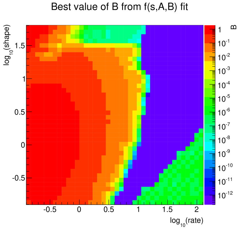
Figure 9: Value of the $B$ parameter for the best fitting function $f(s;A,B)$.

5 Summary and conclusions

The reference prior $\pi(s)$ for the $\text{Poi}(n|s+b)$ model can be computed when an informative prior for the nuisance parameter $b$ is available in the form of a Gamma density with known shape and rate parameters. The reference prior is an improper density, as it can be expected by analogy with Jeffreys’ prior for a single Poisson variable. For practical applications, it is recommended to fix the arbitrary multiplicative constant in such a way that $\pi(s)$ is a monotonically decreasing function with maximum $\pi(0)=1$, as this simplifies the comparison with the widespread uniform prior.

The limiting form of $\pi(s)$ when there is certain information about the backgrond is $\pi_{0}(s)=\sqrt{b_{0}/(s+b_{0})}$, which is Jeffreys’ prior for the offset-ed variable $s^{\prime}=s+b_{0}$. The corresponding posterior $p_{0}(s|n)\propto\text{Ga}(s+b_{0}|n+\frac{1}{2},1)$ provides a valid approximation to the full reference posterior in many cases. In particular, this is true when the relative uncertainty $\sigma[b]/E[b]=1/\sqrt{\alpha}$ on the background in the “signal region” is small, i.e. for large values of the shape parameter $\alpha$. In addition, even when $\alpha$ is small, the approximate prior $\pi_{0}(s)$ differs less than 1% from $\pi(s)$ when the rate parameter $\beta$ is larger than few units.

In most cases, $\pi_{0}(s)$ approximates $\pi(s)$ much better than the uniform prior and the resulting posterior is much simpler. As the Gamma density is available in all software packages used in data analysis, evaluating the approximate reference posterior $p_{0}(s|n)$ is straightforward. When $n$ is not too small (in practice, a few counts are often sufficient), it will provide a very good approximation to the full reference posterior. For these reasons, it is recommended to consider $\pi_{0}(s)$ as the best default or conventional prior, in place of the flat prior, whenever the use of the full reference prior $\pi(s)$ is considered too complicated.

The user shall decide when an approximate form gives acceptable results in her application. In this paper, we adopted an overall agreement not worse than 1% between the priors as a (very conservative) guideline. This implies that, when $\alpha<30$ and $\beta<4$, the full reference prior (or its 2-parameter approximation) should be used. On the other hand, this rule ignores the fact that, unless $n$ is very low or zero, in practice the difference between the corresponding posteriors (the things which matter) is smaller than the difference between priors (and approaches zero when $n$ increases).

The first public implementation of the reference posterior in BAT has also the option of reducing the computing power by means of the 2-parameter function (15), which can reproduce $\pi(s)$ over the entire range of parameters scanned in this work. This option might be useful in applications requiring the evaluation of the reference prior a very large number of times, as the speed-up is at least of three orders of magnitude. People who do not use BAT may implement the same excellent approximation to the reference prior, which is used in BAT to speed-up the computation, by looking at the values of $\pi(s)$ computed for all the points in the background parameters space studied here, as explained in Appendix C.

Appendix A Example with BAT

After installing BAT [10], the BAT/examples/advanced/referencecounting/ folder contains a full example. Here we show that few C++ lines are sufficient to solve a typical problem (see figure 10).

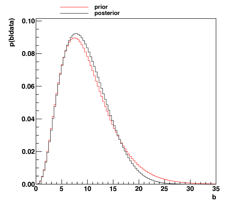
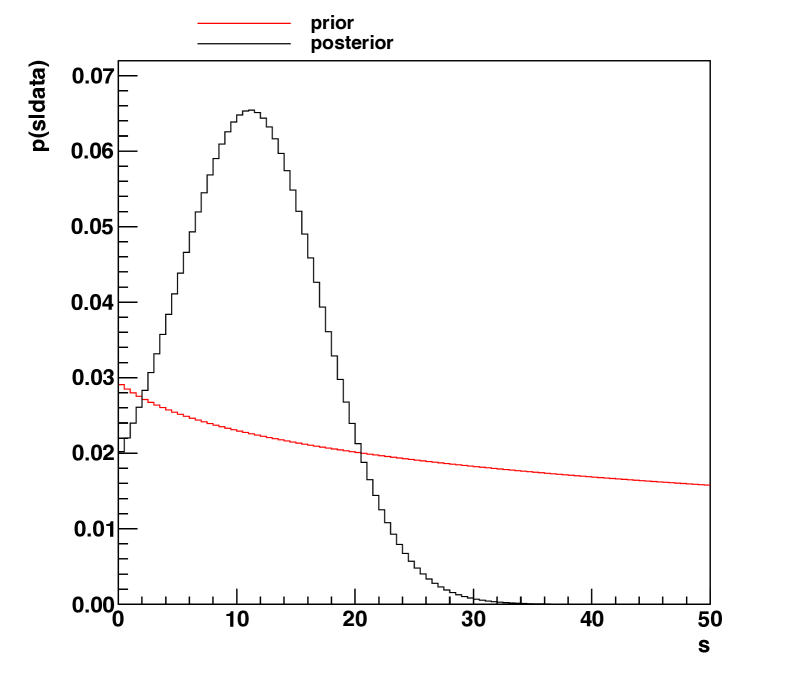
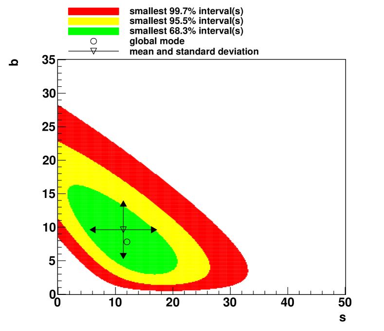
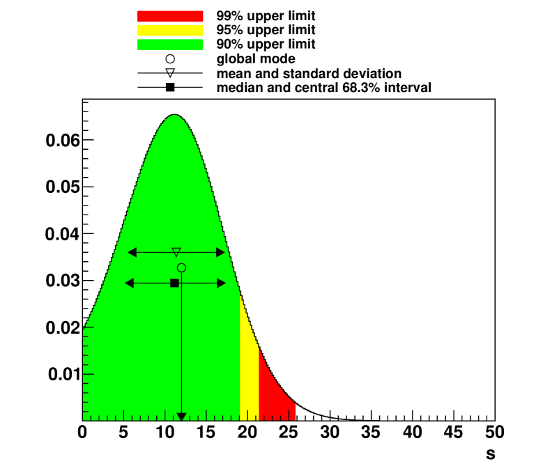
Figure 10: Top: prior and posterior densities of the background (left) and signal (right). Bottom: joint posterior (left) and marginal reference posterior for the signal (right).

  // create new ReferenceCounting object
  ReferenceCounting* m = new ReferenceCounting();

  // BAT settings
  m->SetNbins("s", 300);
  m->SetNbins("b", 300);
  m->MCMCSetPrecision(BCIntegrate::kMedium);

  // set option of how to evaluate prior
  m->SetPriorEvalOption(ReferenceCounting::kHistogram);

  // set background
  double bkg_exp = 10; // expectation value
  double bkg_std = 5;  // uncertainty on background
  double beta    = bkg_exp/bkg_std/bkg_std; // rate
  double alpha   = bkg_exp*beta;            // shape
  m->SetAlphaBeta(alpha, beta);

  // set number of observed events
  m->SetNObs(20);

  // set parameter range
  m->SetParameterRange(0, 0.0, 50); // signal
  m->SetParameterRange(1, 0.0, 35); // background

  // perform sampling with MCMC
  m->MarginalizeAll();

  // perform minimization with Minuit
  m->FindMode( m->GetBestFitParameters() );

  // draw all marginalized distributions
  m->PrintAllMarginalized("plots.pdf");

  // print results of the analysis
  m->PrintResults("results.txt");
 

Appendix B Explicit forms for the marginal posterior

By integrating over $b$ the left- and right-hand terms of the Bayes’ theorem (2) one finds the marginal posterior density for $s$, proportional to the product of the marginal model (7) and the signal prior $p(s)$. The result is similar to (10). Dropping the constant $[\beta/(1+\beta)]^{\alpha}$ we obtain

$$p(s|n)\propto e^{-s}\,f(s;n,\alpha,\beta)\,p(s)$$ (16)

It is simple to show that the marginal model (7) has the form of a linear combination of Gamma kernels. This means that the posterior obtained with the uniform prior is also a mixture of Gamma densities. Its form will be given below.

Here we provide the explicit form for the marginal posterior (16) when the signal prior belongs to the family of Gamma densities. When

$$p(s)=\text{Ga}(s|A,B)$$

it can be shown that the marginal posterior is a linear combination of Gamma densities:

$$p_{A,B}(s|n)=\frac{1}{N}\sum_{m=0}^{n}\binom{\alpha+m-1}{m}\frac{\text{Ga}(s\,|\,n-m+A,1+B)}{(1+\beta)^{m}\,(n-m+A)\,\mathrm{B}(n-m+1,A)}$$ (17)

where the normalization constant is

$$N=\sum_{m=0}^{n}\binom{\alpha+m-1}{m}[(1+\beta)^{m}\,(n-m+A)\,\mathrm{B}(n-m+1,A)]^{-1}$$

with the Beta function $\mathrm{B}(x,y)=\Gamma(x)\Gamma(y)/\Gamma(x+y)$. This result is important for two reasons. First, when there is some prior knowledge about $s$ one should use an informative prior, rather than the reference prior. As for the background, it is best to choose a Gamma density for the signal prior, obtaining the posterior analytically. Second, because the Bayes’ theorem behaves as a linear operator, representing the prior knowledge about $s$ with a linear combination of Gamma densities gives a posterior which is a linear combination of the posteriors computed with each individual Gamma prior. This means that when (17) is used as the prior for the next experiment, one obtains the corresponding posterior with a simple (although tedious) algebra.

The marginal posterior corresponding a flat prior in $s$ can be obtained either by direct computation from the marginal model (7), or from (17) by setting $A=1,B=0$:

$$p_{1,0}(s|n)=\frac{1}{N^{\prime}}\sum_{m=0}^{n}\binom{\alpha+m-1}{m}\frac{\text{Ga}(s\,|\,n-m+1,1)}{(1+\beta)^{m}}$$ (18)

where the normalization constant is

$$N^{\prime}=\sum_{m=0}^{n}\binom{\alpha+m-1}{m}(1+\beta)^{-m}$$

Appendix C Fitting the reference prior to obtain a quick approximation

A text file containing values of $\pi(s)$ at discrete values of $s\in[0,70]$ for all values of the background shape and rate parameters examined in this paper is freely available on Zenodo (10.5281/zenodo.11896). The format of the file is the following.

All lines contain the same number of items, separated by white spaces, such that the file can be considered as a 2-dimensional table. The first row is special, as it provides the header for the table. The first two items in the first row are the strings “shape” and “rate”, which represent the title of the corresponding columns. Next, a number of signal values follows, from $s=0$ to $s=70$ at equally spaced steps. These values are the locations on the positive real line at which the reference prior is computed.

Starting from the second line, the format is always the same. The first two values are the background shape and rate parameters with which the reference prior $\pi(s)$ is defined for the current row. Next, the value $\pi(0)$ (always one) is followed by a fixed number of values $\pi(s_{i})$, where $s_{i}$ is the value at position $i+2$ in the first row, until $\pi(70)$ is given as last value.

The limiting form $\pi_{0}(s)$ only requires the knowledge of the background shape $\alpha$ and rate $\beta$ parameters (first two entries in each row, apart from the first line), as $\pi_{0}(s)=\sqrt{E[b]/(s+E[b])}$ with $E[b]=\alpha/\beta$. To obtain a better approximation, the values of $\pi(s)$ can be fitted by the function (14), or better with (15) where the third parameter can be fixed at $E=0.125$ or $E=0.100$ and initial values for the other two parameters $A,B$ can be set to $E[b]$ and 0 (figure 9 provides more precise indications if the fit does not converge immediately). Of course, the user is free to try different functional forms. For example, a 3-parameter function which well reproduces $\pi(s)$ and is very quick to compute is $\exp(ax^{0.25}+bx^{0.5}+cx)$.

As the shape of $\pi(s)$ changes quite smoothly in the $(\log_{10}\alpha,\log_{10}\beta)$ space (as shown in https://www.youtube.com/watch?v=vqUnRrwinHchttps://www.youtube.com/watch?v=vqUnRrwinHc), the user shall first interpolate the values of $\pi(s)$ computed with the points close to her background parameters (a linear interpolation in the log-log parameters space is enough), before fitting the resulting collection of $\pi(s)$ values.

References

- [1] D. Casadei, Reference analysis of the signal + background model in counting experiments, JINST 7 (2012) P01012, 10.1088/1748-0221/7/01/P01012, \hrefhttp://arXiv.org/abs/1108.4270arXiv: 1108.4270.
- [2] L. Demortier, S. Jain, H.B. Prosper, Reference priors for high energy physics, Phys. Rev. D 82 (2010) 034002.
- [3] M. Pierini, H.B. Prosper, S. Sekmen, M. Spiropulu, Priors for New Physics, 2011, \hrefhttp://arXiv.org/abs/1108.0523arXiv: 1108.0523
- [4] The ATLAS Collaboration, Observation of a new particle in the search for the Standard Model Higgs boson with the ATLAS detector at the LHC, Phys. Lett. B 716 (2012) 1, 10.1016/j.physletb.2012.08.020.
- [5] The CMS Collaboration, Observation of a new boson at a mass of 125 GeV with the CMS experiment at the LHC, Phys. Lett. B 716 (2012) 30, 10.1016/j.physletb.2012.08.021.
- [6] D. Sun and J.O. Berger, Reference priors with partial information, Biometrika 85 (1998) 55, 10.1093/biomet/85.1.55.
- [7] J.M. Bernardo and A.F.M. Smith, Bayesian theory, Wiley, 1994, 10.1002/9780470316870.
- [8] J.M. Bernardo, Reference analysis, in Handbook of Statistics 25 (D.K. Dey, C.R. Rao ed.), Elsevier (2005), pp. 17, 10.1016/S0169-7161(05)25002-2.
- [9] J.O. Berger, J.M. Bernardo, D. Sun, The formal definition of reference priors, The Annals of Statistics 37 (2009) 905, 10.1214/07-AOS587.
- [10] A. Caldwell, D. Kollar, K. Kröninger, BAT - The Bayesian Analysis Toolkit, Computer Physics Communications 180 (2009) 2197-2209 10.1016/j.cpc.2009.06.026, \hrefhttp://arXiv.org/abs/0808.2552arXiv: 0808.2552.