Mechanical Proofs of Properties of the Tribonacci Word

Abstract

We implement a decision procedure for answering questions about a class of infinite words that might be called (for lack of a better name) “Tribonacci-automatic”. This class includes, for example, the famous Tribonacci word ${\bf T}=0102010010201\cdots$, the fixed point of the morphism $0\rightarrow 01$, $1\rightarrow 02$, $2\rightarrow 0$. We use it to reprove some old results about the Tribonacci word from the literature, such as assertions about the occurrences in $\bf T$ of squares, cubes, palindromes, and so forth. We also obtain some new results.

Note: some sections of this paper have been taken, more or less verbatim, from another preprint of the authors and C. F. Du and L. Schaeffer [15].

1 Decidability

As is well-known, the logical theory $\operatorname{Th}({\mathbb{N}},+)$, sometimes called Presburger arithmetic, is decidable [29, 30]. Büchi [7] showed that if we add the function $V_{k}(n)=k^{e}$, for some fixed integer $k\geq 2$, where $e=\max\{i\ :\ k^{i}\,|\,n\}$, then the resulting theory is still decidable. This theory is powerful enough to define finite automata; for a survey, see [6].

As a consequence, we have the following theorem (see, e.g., [33]):

Theorem 1.

There is an algorithm that, given a proposition phrased using only the universal and existential quantifiers, indexing into one or more $k$-automatic sequences, addition, subtraction, logical operations, and comparisons, will decide the truth of that proposition.

Here, by a $k$-automatic sequence, we mean a sequence $\bf a$ computed by deterministic finite automaton with output (DFAO) $M=(Q,\Sigma_{k},\Delta,\delta,q_{0},\kappa)$. Here $\Sigma_{k}:=\{0,1,\ldots,k-1\}$ is the input alphabet, $\Delta$ is the output alphabet, and outputs are associated with the states given by the map $\kappa:Q\rightarrow\Delta$ in the following manner: if $(n)_{k}$ denotes the canonical expansion of $n$ in base $k$, then ${\bf a}[n]=\kappa(\delta(q_{0},(n)_{k}))$. The prototypical example of an automatic sequence is the Thue-Morse sequence ${\bf t}=t_{0}t_{1}t_{2}\cdots$, the fixed point (starting with $0$) of the morphism $0\rightarrow 01$, $1\rightarrow 10$.

It turns out that many results in the literature about properties of automatic sequences, for which some had only long and involved proofs, can be proved purely mechanically using a decision procedure. It suffices to express the property as an appropriate logical predicate, convert the predicate into an automaton accepting representations of integers for which the predicate is true, and examine the automaton. See, for example, the recent papers [1, 22, 24, 23, 25]. Furthermore, in many cases we can explicitly enumerate various aspects of such sequences, such as subword complexity [9].

Beyond base $k$, more exotic numeration systems are known, and one can define automata taking representations in these systems as input. It turns out that in the so-called Pisot numeration systems, addition is computable [16, 17], and hence a theorem analogous to Theorem 1 holds for these systems. See, for example, [5]. It is our contention that the power of this approach has not been widely appreciated, and that many results, previously proved using long and involved ad hoc techniques, can be proved with much less effort by phrasing them as logical predicates and employing a decision procedure. Furthermore, many enumeration questions can be solved with a similar approach.

In a previous paper, we explored the consequences of a decision algorithm for Fibonacci representation [15]. In this paper we discuss our implementation of an analogous algorithm for Tribonacci representation. We use it to reprove some old results from the literature purely mechanically, as well as obtain some new results.

For other works on using computerized formal methods to prove theorems see, for example, [26, 28].

2 Tribonacci representation

Let the Tribonacci numbers be defined, as usual, by the linear recurrence $T_{n}=T_{n-1}+T_{n-2}+T_{n-3}$ for $n\geq 3$ with initial values $T_{0}=0$, $T_{1}=1$, $T_{2}=1$. (We caution the reader that some authors use a different indexing for these numbers.) Here are the first few values of this sequence.

$n$	0	1	2	3	4	5	6	7	8	9	10	11	12	13	14	15	16
$T_{n}$	0	1	1	2	4	7	13	24	44	81	149	274	504	927	1705	3136	5768

From the theory of linear recurrences we know that

$$T_{n}=c_{1}\alpha^{n}+c_{2}\beta^{n}+c_{3}\gamma^{n}$$

where $\alpha,\beta,\gamma$ are the zeros of the polynomial $x^{3}-x^{2}-x-1$. The only real zero is $\alpha\doteq 1.83928675521416113255185$; the other two zeros are complex and are of magnitude $<3/4$. Solving for the constants, we find that $c_{1}\doteq 0.336228116994941094225362954$, the real zero of the polynomial $44x^{3}-2x-1=0$. It follows that $T_{n}=c_{1}\alpha^{n}+O(.75^{n})$. In particular $T_{n}/T_{n-1}=\alpha+O(.41^{n})$.

It is well-known that every non-negative integer can be represented, in an essentially unique way, as a sum of Tribonacci numbers $(T_{i})_{i\geq 2}$, subject to the constraint that no three consecutive Tribonacci numbers are used [8]. For example, $43=T_{7}+T_{6}+T_{4}+T_{3}$.

Such a representation can be written as a binary word $a_{1}a_{2}\cdots a_{n}$ representing the integer $\sum_{1\leq i\leq n}a_{i}T_{n+2-i}$. For example, the binary word $110110$ is the Tribonacci representation of $43$.

For $w=a_{1}a_{2}\cdots a_{n}\in\Sigma_{2}^{*}$, we define $[a_{1}a_{2}\cdots a_{n}]_{T}:=\sum_{1\leq i\leq n}a_{i}T_{n+2-i}$, even if $a_{1}a_{2}\cdots a_{n}$ has leading zeros or occurrences of the word $111$.

By $(n)_{T}$ we mean the canonical Tribonacci representation for the integer $n$, having no leading zeros or occurrences of $111$. Note that $(0)_{T}=\epsilon$, the empty word. The language of all canonical representations of elements of ${\mathbb{N}}$ is $\epsilon+(1+11)(0+01+011)^{*}$.

Just as Tribonacci representation is an analogue of base-$k$ representation, we can define the notion of Tribonacci-automatic sequence as the analogue of the more familiar notation of $k$-automatic sequence [12, 2]. We say that an infinite word ${\bf a}=(a_{n})_{n\geq 0}$ is Tribonacci-automatic if there exists an automaton with output $M=(Q,\Sigma_{2},q_{0},\delta,\kappa,\Delta)$ that $a_{n}=\kappa(\delta(q_{0},(n)_{T}))$ for all $n\geq 0$. An example of a Tribonacci-automatic sequence is the infinite Tribonacci word,

$${\bf T}=T_{0}T_{1}T_{2}\cdots=0102010010201\cdots$$

which is generated by the following 3-state automaton:

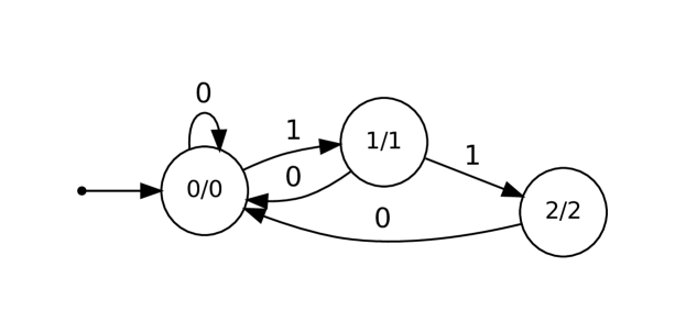
Figure 1: Automaton generating the Tribonacci sequence

To compute $T_{i}$, we express $i$ in canonical Tribonacci representation, and feed it into the automaton. Then $T_{i}$ is the output associated with the last state reached (denoted by the symbol after the slash).

A basic fact about Tribonacci representation is that addition can be performed by a finite automaton. To make this precise, we need to generalize our notion of Tribonacci representation to $r$-tuples of integers for $r\geq 1$. A representation for $(x_{1},x_{2},\ldots,x_{r})$ consists of a string of symbols $z$ over the alphabet $\Sigma_{2}^{r}$, such that the projection $\pi_{i}(z)$ over the $i$’th coordinate gives a Tribonacci representation of $x_{i}$. Notice that since the canonical Tribonacci representations of the individual $x_{i}$ may have different lengths, padding with leading zeros will often be necessary. A representation for $(x_{1},x_{2},\ldots,x_{r})$ is called canonical if it has no leading $[0,0,\ldots 0]$ symbols and the projections into individual coordinates have no occurrences of $111$. We write the canonical representation as $(x_{1},x_{2},\ldots,x_{r})_{T}$. Thus, for example, the canonical representation for $(9,16)$ is $[0,1][1,0][0,0][1,1][0,1]$.

Thus, our claim about addition in Tribonacci representation is that there exists a deterministic finite automaton (DFA) $M_{\rm add}$ that takes input words of the form $[0,0,0]^{*}(x,y,z)_{T}$, and accepts if and only if $x+y=z$. Thus, for example, $M_{\rm add}$ accepts $[1,0,1][0,1,1][0,0,0]$ since the three words obtained by projection are $100$, $010$, and $110$, which represent, respectively, $4$, $2$, and $6$ in Tribonacci representation.

Since this automaton does not appear to have been given explicitly in the literature and it is essential to our implementation, we give it here. This automaton actually works even for non-canonical expansions having three consecutive $1$’s. The initial state is state $1$. The state $0$ is a “dead state” that can safely be ignored.

We briefly sketch a proof of the correctness of this automaton. States can be identified with certain sequences, as follows: if $x,y,z$ are the identical-length words arising from projection of a word that takes $M_{\rm add}$ from the initial state $1$ to the state $t$, then $t$ is identified with the integer sequence $([x0^{n}]_{T}+[y0^{n}]_{T}-[z0^{n}]_{T})_{n\geq 0}$. State $0$ corresponds to sequences that can never lead to $0$, as they are too positive or too negative.

When we intersect this automaton with the appropriate regular language (ruling out input triples containing $111$ in any coordinate), we get an automaton with 149 states accepting $0^{*}(x,y,z)_{T}$ such that $x+y=z$.

Another basic fact about Tribonacci representation is that, for canonical representations containing no three consecutive $1$’s or leading zeros, the radix order on representations is the same as the ordinary ordering on ${\mathbb{N}}$. It follows that a very simple automaton can, on input $(x,y)_{T}$, decide whether $x<y$.

Putting this all together, we get the analogue of Theorem 1:

Procedure 2 (Decision procedure for Tribonacci-automatic words).

Input:

• $m,n\in{\mathbb{N}}$;

• $m$ DFAOs generating the Tribonacci-automatic words ${\bf w}_{1},{\bf w}_{2},\dots,{\bf w}_{m}$;

• a first-order proposition with $n$ free variables $\varphi(v_{1},v_{2},\dots,v_{n})$ using constants and relations definable in $\operatorname{Th}({\mathbb{N}},0,1,+)$ and indexing into ${\bf w}_{1},{\bf w}_{2},\dots,{\bf w}_{m}$.

Output: DFA with input alphabet $\Sigma_{2}^{n}$ accepting $\{(k_{1},k_{2},\dots,k_{n})_{T}\;:\;\varphi(k_{1},k_{2},\dots,k_{n})\text{ holds}\}$.

$q$	[0,0,0]	[0,0,1]	[0,1,0]	[0,1,1]	[1,0,0]	[1,0,1]	[1,1,0]	[1,1,1]	acc/rej
0	0	0	0	0	0	0	0	0	0
1	1	2	3	1	3	1	0	3	1
2	4	0	5	4	5	4	6	5	0
3	0	7	0	0	0	0	0	0	0
4	0	0	0	0	0	0	8	0	0
5	9	0	10	9	10	9	11	10	0
6	12	13	0	12	0	12	0	0	1
7	0	14	0	0	0	0	0	0	0
8	0	0	9	0	9	0	10	9	0
9	0	0	4	0	4	0	5	4	0
10	2	15	1	2	1	2	3	1	0
11	7	16	0	7	0	7	0	0	1
12	14	17	0	14	0	14	0	0	1
13	18	19	20	18	20	18	21	20	0
14	3	1	0	3	0	3	0	0	0
15	0	0	0	0	0	0	22	0	0
16	20	18	21	20	21	20	0	21	1
17	5	4	6	5	6	5	23	6	1
18	0	0	8	0	8	0	24	8	0
19	0	0	0	0	0	0	25	0	0
20	10	9	11	10	11	10	0	11	1
21	0	12	0	0	0	0	0	0	0
22	0	0	26	0	26	0	27	26	0
23	0	28	0	0	0	0	0	0	0
24	13	29	12	13	12	13	0	12	0
25	0	0	0	0	0	0	26	0	0
26	0	0	0	0	0	0	4	0	0
27	15	0	2	15	2	15	1	2	0
28	0	30	0	0	0	0	0	0	0
29	0	0	31	0	31	0	32	31	0
30	0	3	0	0	0	0	0	0	0
31	0	0	0	0	0	0	33	0	0
32	26	0	27	26	27	26	34	27	0
33	0	0	0	0	0	0	9	0	0
34	16	35	7	16	7	16	0	7	0
35	31	0	32	31	32	31	36	32	0
36	37	38	39	37	39	37	0	39	1
37	17	40	14	17	14	17	0	14	0
38	19	0	18	19	18	19	20	18	0
39	0	41	0	0	0	0	0	0	1
40	0	0	22	0	22	0	42	22	0
41	21	20	0	21	0	21	0	0	0
42	38	43	37	38	37	38	39	37	0
43	0	0	0	0	0	0	31	0	0

Table 1: Transition table for $M_{\rm add}$ for Tribonacci addition

3 Mechanical proofs of properties of the infinite Tribonacci word

Recall that a word $x$, whether finite or infinite, is said to have period $p$ if $x[i]=x[i+p]$ for all $i$ for which this equality is meaningful. Thus, for example, the English word ${\tt alfalfa}$ has period $3$. The exponent of a finite word $x$, written $\exp(x)$, is $|x|/P$, where $P$ is the smallest period of $x$. Thus $\exp({\tt alfalfa})=7/3$.

If $\bf x$ is an infinite word with a finite period, we say it is ultimately periodic. An infinite word $\bf x$ is ultimately periodic if and only if there are finite words $u,v$ such that $x=uv^{\omega}$, where $v^{\omega}=vvv\cdots$.

A nonempty word of the form $xx$ is called a square, and a nonempty word of the form $xxx$ is called a cube. More generally, a nonempty word of the form $x^{n}$ is called an $n$’th power. By the order of a square $xx$, cube $xxx$, or $n$’th power $x^{n}$, we mean the length $|x|$.

The infinite Tribonacci word ${\bf T}=0102010\cdots=T_{0}T_{1}T_{2}\cdots$ can be described in many different ways. In addition to our definition in terms of automata, it is also the fixed point of the morphism $\varphi(0)=01$, $\varphi(1)=02$, and $\varphi(1)=0$. This word has been studied extensively in the literature; see, for example, [10, 3, 32, 18, 34, 14, 31, 35].

It can also be described as the limit of the finite Tribonacci words $(Y_{n})_{n\geq 0}$, defined as follows:

$$Y_{0} =\epsilon$$

$$Y_{1} =2$$

$$Y_{2} =0$$

$$Y_{3} =01$$

$$Y_{n} =Y_{n-1}Y_{n-2}Y_{n-3}\ \text{for $n\geq 4$}.$$

Note that $Y_{n}$, for $n\geq 2$, is the prefix of length $T_{n}$ of $\bf T$.

In the next subsection, we use our implementation to prove a variety of results about repetitions in $\bf T$.

3.1 Repetitions

It is known that all strict epistandard words (or Arnoux-Rauzy words), are not ultimately periodic (see, for example, [20]). Since $\bf T$ is in this class, we have the following known result which we can reprove using our method.

Theorem 3.

The word $\bf T$ is not ultimately periodic.

Proof.

We construct a predicate asserting that the integer $p\geq 1$ is a period of some suffix of $\bf T$:

$$(p\geq 1)\ \wedge\ \exists n\ \forall i\geq n\ {\bf T}[i]={\bf T}[i+p].$$

(Note: unless otherwise indicated, whenever we refer to a variable in a predicate, the range of the variable is assumed to be ${\mathbb{N}}=\{0,1,2,\ldots\}$.) From this predicate, using our program, we constructed an automaton accepting the language

$$L=0^{*}\ \{(p)_{T}\ :\ (p\geq 1)\ \wedge\ \exists n\ \forall i\geq n\ {\bf T}[i]={\bf T}[i+p]\}.$$

This automaton accepts the empty language, and so it follows that ${\bf T}$ is not ultimately periodic.

Here is the log of our program:

p >= 1 with 5 states, in 426ms
 i >= n with 13 states, in 3ms
  i + p with 150 states, in 31ms
   TR[i] = TR[i + p] with 102 states, in 225ms
    i >= n => TR[i] = TR[i + p] with 518 states, in 121ms
     Ai i >= n => TR[i] = TR[i + p] with 4 states, in 1098ms
      En Ai i >= n => TR[i] = TR[i + p] with 2 states, in 0ms
       p >= 1 & En Ai i >= n => TR[i] = TR[i + p] with 2 states, in 1ms
overall time: 1905ms

The largest intermediate automaton during the computation had 5999 states.

A few words of explanation are in order: here “T” refers to the sequence $\bf T$, and “E” is our abbreviation for $\exists$ and “A” is our abbreviation for $\forall$. The symbol “=>” is logical implication, and “&” is logical and. ∎

From now on, whenever we discuss the language accepted by an automaton, we will omit the $0^{*}$ at the beginning.

We now turn to repetitions. As a particular case of [18, Thm. 6.31 and Example 7.6, p. 130] and [19, Example 6.21] we have the following result, which we can reprove using our method.

Theorem 4.

$\bf T$ contains no fourth powers.

Proof.

A natural predicate for the orders of all fourth powers occurring in $\bf T$:

$$(n>0)\ \wedge\ \exists i\ \forall t<3n\ {\bf T}[i+t]={\bf T}[i+n+t].$$

However, this predicate could not be run on our prover. It runs out of space while trying to determinize an NFA with 24904 states.

Instead, we make the substitution $j=i+t$, obtaining the new predicate

$$(n>0)\ \wedge\ \exists i\ \forall j\ ((j\geq i)\wedge(j<i+3n))\implies{\bf T}[j]={\bf T}[j+n].$$

The resulting automaton accepts nothing, so there are no fourth powers.

Here is the log.

n > 0 with 5 states, in 59ms
 i <= j with 13 states, in 15ms
  3 * n with 147 states, in 423ms
   i + 3 * n with 799 states, in 4397ms
    j < i + 3 * n with 1103 states, in 4003ms
     i <= j & j < i + 3 * n with 1115 states, in 111ms
      j + n with 150 states, in 18ms
       TR[j] = TR[j + n] with 102 states, in 76ms
        i <= j & j < i + 3 * n => TR[j] = TR[j + n] with 6550 states, in 1742ms
         Aj i <= j & j < i + 3 * n => TR[j] = TR[j + n] with 4 states, in 69057ms
          Ei Aj i <= j & j < i + 3 * n => TR[j] = TR[j + n] with 2 states, in 0ms
           n > 0 & Ei Aj i <= j & j < i + 3 * n => TR[j] = TR[j + n] with 2 states, in 0ms
overall time: 79901ms

The largest intermediate automaton in the computation had 86711 states. ∎

Next, we move on to a description of the orders of squares occurring in $\bf T$. We reprove a result of Glen [18, §6.3.5].

Theorem 5.

All squares in $\bf T$ are of order $T_{n}$ or $T_{n}+T_{n-1}$ for some $n\geq 2$. Furthermore, for all $n\geq 2$, there exists a square of order $T_{n}$ and $T_{n}+T_{n-1}$ in $\bf T$.

Proof.

A natural predicate for the lengths of squares is

$$(n>0)\ \wedge\ \exists i\ \forall t<n\ {\bf T}[i+t]={\bf T}[i+n+t].$$

but when we run our solver on this predicate, we get an intermediate NFA of 4612 states that our solver could not determinize in the the allotted space. The problem appears to arise from the three different variables indexing $T$. To get around this problem, we rephrase the predicate, introducing a new variable $j$ that represents $i+t$. This gives the predicate

$$(n>0)\ \wedge\ \exists i\ \forall j\ ((i\leq j)\wedge(j<i+n))\implies{\bf T}[j]={\bf T}[j+n].$$

and the following log

i <= j with 13 states, in 10ms
 i + n with 150 states, in 88ms
  j < i + n with 229 states, in 652ms
   i <= j & j < i + n with 241 states, in 42ms
    j + n with 150 states, in 19ms
     TR[j] = TR[j + n] with 102 states, in 61ms
      i <= j & j < i + n => TR[j] = TR[j + n] with 1751 states, in 341ms
       Aj i <= j & j < i + n => TR[j] = TR[j + n] with 11 states, in 4963ms
        Ei Aj i <= j & j < i + n => TR[j] = TR[j + n] with 4 states, in 4ms
         n > 0 & Ei Aj i <= j & j < i + n => TR[j] = TR[j + n] with 4 states, in 0ms
overall time: 6232ms

The resulting automaton accepts exactly the language $10^{*}+110^{*}$. The largest intermediate automaton had 26949 states. ∎

We can easily get more information about the square occurrences in $\bf T$. By modifying our previous predicate, we get

$$(n>0)\ \wedge\ \forall j\ ((i\leq j)\wedge(j<i+n))\implies{\bf T}[j]={\bf T}[j+n]$$

which encodes those $(i,n)$ pairs such that there is a square of order $n$ beginning at position $i$ of $\bf T$.

This automaton has only 10 states and efficiently encodes the orders and starting positions of each square in $\bf T$. During the computation, the largest intermediate automaton had 26949 states. Thus we have proved

Theorem 6.

The language

$$\{(i,n)_{T}\ :\ \text{there is a square of order $n$ beginning at position $i$ in {\bf T}}\}$$

is accepted by the automaton in Figure 2.

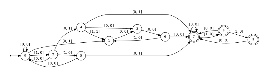
Figure 2: Automaton accepting orders and positions of all squares in $\bf T$

Next, we examine the cubes in $\bf T$. Evidently Theorem 5 implies that any cube in $\bf T$ must be of order $T_{n}$ or $T_{n}+T_{n-1}$ for some $n$. However, not every order occurs. We thus recover the following result of Glen [18, §6.3.7].

Theorem 7.

The cubes in $\bf T$ are of order $T_{n}$ for $n\geq 5$, and a cube of each such order occurs.

Proof.

We use the predicate

$$(n>0)\ \wedge\ \exists i\ \forall j\ ((i\leq j)\wedge(j<i+2n))\implies{\bf T}[j]={\bf T}[j+n].$$

When we run our program, we obtain an automaton accepting exactly the language $(1000)0^{*}$, which corresponds to $T_{n}$ for $n\geq 5$.

The largest intermediate automaton had 60743 states. ∎

Next, we encode the orders and positions of all cubes. We build a DFA accepting the language

$$\{(i,n)_{T}\ :\ (n>0)\ \wedge\ \forall j\ ((i\leq j)\wedge(j<i+2n))\implies{\bf T}[j]={\bf T}[j+n]\}.$$

Theorem 8.

The language

$$\{(n,i)_{T}\ :\ \text{there is a cube of order $n$ beginning at position $i$ in {\bf T}}\}$$

is accepted by the automaton in Figure 3.

Figure 3: Automaton accepting orders and positions of all cubes in $\bf T$

We also computed an automaton accepting those pairs $(p,n)$ such that there is a factor of $\bf T$ having length $n$ and period $p$, and $n$ is the largest such length corresponding to the period $p$. However, this automaton has 266 states, so we do not give it here.

3.2 Palindromes

We now turn to a characterization of the palindromes in $\bf T$. Once again it turns out that the predicate we previously used in [15], namely,

$$\exists i\ \forall j<n\ {\bf T}[i+j]={\bf T}[i+n-1-j],$$

resulted in an intermediate NFA of 5711 states that we could not successfully determinize.

Instead, we used two equivalent predicates. The first accepts $n$ if there is an even-length palindrome, of length $2n$, centered at position $i$:

$$\exists i\geq n\ \forall j<n\ {\bf T}[i+j]={\bf T}[i-j-1].$$

The second accepts $n$ if there is an odd-length palindrome, of length $2n+1$, centered at position $i$:

$$\exists i\geq n\ \forall j\ (1\leq j\leq n)\implies{\bf T}[i+j]={\bf T}[i-j].$$

Theorem 9.

There exist palindromes of every length $\geq 0$ in $\bf T$.

Proof.

For the first predicate, our program outputs the automaton below. It clearly accepts the Tribonacci representations for all $n$.

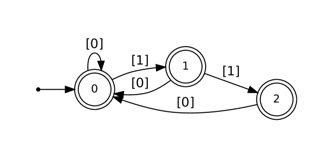
Figure 4: Automaton accepting lengths of palindromes in $\bf T$

The log of our program follows.

i >= n with 13 states, in 34ms
 j < n with 13 states, in 8ms
  i + j with 150 states, in 53ms
   i - 1 with 7 states, in 155ms
    i - 1 - j with 150 states, in 166ms
     TR[i + j] = TR[i - 1 - j] with 664 states, in 723ms
      j < n => TR[i + j] = TR[i - 1 - j] with 3312 states, in 669ms
       Aj j < n => TR[i + j] = TR[i - 1 - j] with 24 states, in 5782274ms
        i >= n & Aj j < n => TR[i + j] = TR[i - 1 - j] with 24 states, in 0ms
         Ei i >= n & Aj j < n => TR[i + j] = TR[i - 1 - j] with 4 states, in 6ms
overall time: 5784088ms

The largest intermediate automaton had 918871 states. This was a fairly significant computation, taking about two hours’ CPU time on a laptop.

We omit the details of the computation for the odd-length palindromes, which are quite similar. ∎

Remark 10.

A. Glen has pointed out to us that this follows from the fact that $\bf T$ is episturmian and hence rich, so a new palindrome is introduced at each new position in $T$.

We could also characterize the positions of all nonempty palindromes. To illustrate the idea, we generated an automaton accepting $(i,n)$ such that ${\bf T}[i-n..i+n-1]$ is an (even-length) palindrome.

Figure 5: Automaton accepting orders and positions of all nonempty even-length palindromes in $\bf T$

The prefixes are factors of particular interest. Let us determine which prefixes are palindromes:

Theorem 11.

The prefix ${\bf T}[0..n-1]$ of length $n$ is a palindrome if and only if $n=0$ or $(n)_{T}\in 1+11+10(010)^{*}(00+001+0011)$.

Proof.

We use the predicate

$$\forall i<n\ {\bf T}[i]={\bf T}[n-1-i].$$

The automaton generated is given below.

Figure 6: Automaton accepting lengths of palindromes in $\bf T$

∎

Remark 12.

A. Glen points out to us that the palindromic prefixes of $\bf T$ are precisely those of the form $\operatorname{Pal}(w)$, where $w$ is a finite prefix of the infinite word $(012)^{\omega}$ and $\operatorname{Pal}$ denotes the “iterated palindromic closure”; see, for example, [20, Example 2.6]. She also points out that these lengths are precisely the integers $(T_{i}+T_{i+2}-3)/2$ for $i\geq 1$.

3.3 Quasiperiods

We now turn to quasiperiods. An infinite word $\bf a$ is said to be quasiperiodic if there is some finite nonempty word $x$ such that ${\bf a}$ can be completely “covered” with translates of $x$. Here we study the stronger version of quasiperiodicity where the first copy of $x$ used must be aligned with the left edge of $\bf w$ and is not allowed to “hang over”; these are called aligned covers in [11]. More precisely, for us ${\bf a}=a_{0}a_{1}a_{2}\cdots$ is quasiperiodic if there exists $x$ such that for all $i\geq 0$ there exists $j\geq 0$ with $i-n<j\leq i$ such that $a_{j}a_{j+1}\cdots a_{j+n-1}=x$, where $n=|x|$. Such an $x$ is called a quasiperiod. Note that the condition $j\geq 0$ implies that, in this interpretation, any quasiperiod must actually be a prefix of $\bf a$.

Glen, Levé, and Richomme characterized the quasiperiods of a large class of words, including the Tribonacci word [21, Thm. 4.19]. However, their characterization did not explicitly give the lengths of the quasiperiods. We do that in the following result.

Theorem 13.

A nonempty length-$n$ prefix of $\bf T$ is a quasiperiod of $\bf T$ if and only if $n$ is accepted by the following automaton:

Figure 7: Automaton accepting lengths of quasiperiods of the Tribonacci sequence

Proof.

We write a predicate for the assertion that the length-$n$ prefix is a quasiperiod:

$$\forall i\geq 0\ \exists j\text{ with }i-n<j\leq i\text{ such that }\forall t<n\ {\bf T}[t]={\bf T}[j+t].$$

When we do this, we get the automaton above. These numbers are those $i$ for which $T_{n}\leq i\leq U_{n}$ for $n\geq 5$, where $U_{2}=0$, $U_{3}=1$, $U_{4}=3$, and $U_{n}=U_{n-1}+U_{n-2}+U_{n-3}+3$ for $n\geq 5$. ∎

3.4 Unbordered factors

Next we look at unbordered factors. A word $y$ is said to be a border of $x$ if $y$ is both a nonempty proper prefix and suffix of $x$. A word $x$ is bordered if it has at least one border. It is easy to see that if a word $y$ is bordered iff it has a border of length $\ell$ with $0<\ell\leq|y|/2$.

Theorem 14.

There is an unbordered factor of length $n$ of $\bf T$ if and only if $(n)_{T}$ is accepted by the automaton given below.

Figure 8: Automaton accepting lengths of unbordered factors of the Tribonacci sequence

Proof.

As in a previous paper [15] we can express the property of having an unbordered factor of length $n$ as follows

$$\exists i\ \forall j,1\leq j\leq n/2,\ \exists t<j\ {\bf T}[i+t]\not={\bf T}[i+n-j+t].$$

However, this does not run to completion within the available space on our prover. Instead, make the substitutions $t^{\prime}=n-j$ and $u=i+t$. This gives the predicate

$$\exists i\ \forall t^{\prime},\ n/2\leq t^{\prime}<n,\ \exists u,\ (i\leq u<i+n-t^{\prime})\ {\bf T}[u]\not={\bf T}[u+t^{\prime}].$$

Here is the log:

2 * t with 61 states, in 276ms
n <= 2 * t with 79 states, in 216ms
t < n with 13 states, in 3ms
n <= 2 * t & t < n with 83 states, in 9ms
u >= i with 13 states, in 7ms
i + n with 150 states, in 27ms
i + n - t with 1088 states, in 7365ms
u < i + n - t with 1486 states, in 6041ms
u >= i & u < i + n - t with 1540 states, in 275ms
u + t with 150 states, in 5ms
TR[u] != TR[u + t] with 102 states, in 22ms
u >= i & u < i + n - t & TR[u] != TR[u + t] with 7489 states, in 3364ms
Eu u >= i & u < i + n - t & TR[u] != TR[u + t] with 552 states, in 5246873ms
n <= 2 * t & t < n => Eu u >= i & u < i + n - t & TR[u] != TR[u + t] with 944 states, in 38ms
At n <= 2 * t & t < n => Eu u >= i & u < i + n - t & TR[u] != TR[u + t] with 47 states, in 1184ms
Ei At n <= 2 * t & t < n => Eu u >= i & u < i + n - t & TR[u] != TR[u + t] with 25 states, in 2ms
overall time: 5265707ms

∎

3.5 Lyndon words

Next, we turn to some results about Lyndon words. Recall that a nonempty word $x$ is a Lyndon word if it is lexicographically less than all of its nonempty proper prefixes.

Theorem 15.

There is a factor of length $n$ of $\bf T$ that is Lyndon if and only if $n$ is accepted by the automaton given below.

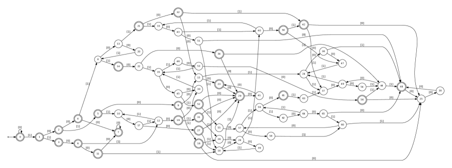
Figure 9: Automaton accepting lengths of Lyndon factors of the Tribonacci sequence

Proof.

Here is a predicate specifying that there is a factor of length $n$ that is Lyndon:

$$\exists i\ \forall j,1\leq j<n,\ \exists t<n-j\ (\forall u<t\ {\bf T}[i+u]={\bf T}[i+j+u])\ \wedge\ {\bf T}[i+t]<{\bf T}[i+j+t].$$

Unfortunately this predicate did not run to completion, so we substituted $u^{\prime}:=i+u$ to get

$$\exists i\ \forall j,1\leq j<n,\ \exists t<n-j\ (\forall u^{\prime},i\leq u^{\prime}<i+t\ {\bf T}[u^{\prime}]={\bf T}[u^{\prime}+j])\ \wedge\ {\bf T}[i+t]<{\bf T}[i+j+t].$$

∎

3.6 Critical exponent

Recall from Section 3 that $\exp(w)=|w|/P$, where $P$ is the smallest period of $w$. The critical exponent of an infinite word $\bf x$ is the supremum, over all factors $w$ of $\bf x$, of $\exp(w)$.

Then Tan and Wen [34] proved that

Theorem 16.

The critical exponent of $\bf T$ is $\rho\doteq 3.19148788395311874706$, the real zero of the polynomial $2x^{3}-12x^{2}+22x-13$.

A. Glen points out that this result can also be deduced from [27, Thm. 5.2].

Proof.

Let $x$ be any factor of exponent $\geq 3$ in $\bf T$. From Theorem 3 we know that such $x$ exist. Let $n=|x|$ and $p$ be the period, so that $n/p\geq 3$. Then by considering the first $3p$ symbols of $x$, which form a cube, we have by Theorem 3 that $p=T_{n}$. So it suffices to determine the largest $n$ corresponding to every $p$ of the form $T_{n}$. We did this using the predicate

Figure 10: Length $n$ of longest factors having period $p=T_{n}$ of Tribonacci sequence

From inspection of the automaton, we see that the maximum length of a factor $n=U_{j}$ having period $p=T_{j}$, $j\geq 2$, is given by

$$U_{j}=\begin{cases}2,&\text{if $j=2$};\\ 5,&\text{if $j=3$};\\ [110(100)^{i-1}0]_{T},&\text{if $j=3i+1\geq 4$};\\ [110(100)^{i-1}01]_{T},&\text{if $j=3i+2\geq 5$};\\ [110(100)^{i-1}011]_{T},&\text{if $j=3i+3\geq 6$}.\end{cases}$$

A tedious induction shows that $U_{j}$ satisfies the linear recurrence $U_{j}=U_{j-1}+U_{j-2}+U_{j-3}+3$ for $j\geq 5$. Hence we can write $U_{j}$ as a linear combination Tribonacci sequences and the constant sequence $1$, and solving for the constants we get

$$U_{j}={5\over 2}T_{j}+T_{j-1}+{1\over 2}T_{j-2}-{3\over 2}$$

for $j\geq 2$.

The critical exponent of $T$ is then $\sup_{j\geq 1}U_{j}/T_{j}$. Now

$$U_{j}/T_{j} ={5\over 2}+{{T_{j-1}}\over{T_{j}}}+{{T_{j-2}}\over{2T_{j}}}-{3\over{2T_{j}}}$$

$$={5\over 2}+\alpha^{-1}+{1\over 2}\alpha^{-2}+O(1.8^{-j}).$$

Hence $U_{j}/T_{j}$ tends to $5/2+\alpha^{-1}+{1\over 2}\alpha^{-2}=\rho$. ∎

We can also ask the same sort of questions about the initial critical exponent of a word $\bf w$, which is the supremum over the exponents of all prefixes of $\bf w$.

Theorem 17.

The initial critical exponent of $\bf T$ is $\rho-1$.

Proof.

We create an automaton $M_{\rm ice}$ accepting the language

$$L=\{(n,p)_{T}\ :\ {\bf T}[0..n-1]\text{ has least period }p\}.$$

It is depicted in Figure 11 below. An analysis similar to that we gave above for the critical exponent gives the result.

Figure 11: Automaton accepting least periods of prefixes of length $n$

∎

Recall that a primitive word is a non-power; that is, a word that cannot be written in the form $x^{n}$ where $n$ is an integer $\geq 2$.

Theorem 18.

The only prefixes of the Tribonacci word that are powers are those of length $2T_{n}$ for $n\geq 5$.

Proof.

The predicate

$$\exists d<n\ (\forall j<n-d\ {\bf T}[j]={\bf T}[d+j])\ \wedge\ (\forall k<d\ {\bf T}[k]={\bf T}[n-d+k])$$

asserts that the prefix ${\bf T}[0..n-1]$ is a power. When we run this through our program, the resulting automaton accepts $100010^{*}$, which corresponds to $F_{n+1}+F_{n-3}=2T_{n}$ for $n\geq 5$. ∎

4 Enumeration

Mimicking the base-$k$ ideas in [9], we can also mechanically enumerate many aspects of Tribonacci-automatic sequences. We do this by encoding the factors having the property in terms of paths of an automaton. This gives the concept of Tribonacci-regular sequence Roughly speaking, a sequence $(a(n))_{n\geq 0}$ taking values in ${\mathbb{N}}$ is Tribonacci-regular if the set of sequences

$$\{(a([xw]_{T})_{w\in\Sigma_{2}^{*}}\ :\ x\in\Sigma_{2}^{*}\}$$

is finitely generated. Here we assume that $a([xw]_{T})$ evaluates to $0$ if $xw$ contains the word $111$. Every Tribonacci-regular sequence $(a(n))_{n\geq 0}$ has a linear representation of the form $(u,\mu,v)$ where $u$ and $v$ are row and column vectors, respectively, and $\mu:\Sigma_{2}\rightarrow{\mathbb{N}}^{d\times d}$ is a matrix-valued morphism, where $\mu(0)=M_{0}$ and $\mu(1)=M_{1}$ are $d\times d$ matrices for some $d\geq 1$, such that

$$a(n)=u\cdot\mu(x)\cdot v$$

whenever $[x]_{T}=n$. The rank of the representation is the integer $d$.

Recall that if $\bf x$ is an infinite word, then the subword complexity function $\rho_{\bf x}(n)$ counts the number of distinct factors of length $n$. Then, in analogy with [9, Thm. 27], we have

Theorem 19.

If $\bf x$ is Tribonacci-automatic, then the subword complexity function of $\bf x$ is Tribonacci-regular.

Using our implementation, we can obtain a linear representation of the subword complexity function for $\bf T$. An obvious choice is to use the language

$$\{(n,i)_{T}\ :\ \forall j<i\ {\bf T}[i..i+n-1]\not={\bf T}[j..j+n-1]\},$$

based on a predicate that expresses the assertion that the factor of length $n$ beginning at position $i$ has never appeared before. Then, for each $n$, the number of corresponding $i$ gives $\rho_{\bf T}(n)$.

However, this does not run to completion in our implementation in the allotted time and space. Instead, let us substitute $u=j+t$ and and $k=i-j$ to get the predicate

$$\forall k\ (((k>0)\wedge(k\leq i))\implies(\exists u\ ((u\geq j)\wedge(u<n+j)\wedge({\bf T}[u]\not={\bf T}[u+k])))).$$

This predicate is close to the upper limit of what we can compute using our program. The largest intermediate automaton had 1230379 states and the program took 12323.82 seconds, giving us a linear representation $(u,\mu,v)$ rank $22$. When we minimize this using the algorithm in [4] we get the rank-$12$ linear representation

$$u =[1\ 0\ 0\ 0\ 0\ 0\ 0\ 0\ 0\ 0\ 0\ 0]$$

$$M_{0} =\left[\begin{array}[]{cccccccccccc}1&0&0&0&0&0&0&0&0&0&0&0\\ 0&0&1&0&0&0&0&0&0&0&0&0\\ 0&0&0&0&1&0&0&0&0&0&0&0\\ -1&0&1&0&1&0&0&0&0&0&0&0\\ 0&0&0&0&0&0&1&0&0&0&0&0\\ -1&0&1&0&0&0&1&0&0&0&0&0\\ -2&0&1&0&1&0&1&0&0&0&0&0\\ -3&0&2&0&1&0&1&0&0&0&0&0\\ -4&0&2&0&2&0&1&0&0&0&0&0\\ -5&0&2&0&2&0&2&0&0&0&0&0\\ -6&0&2&0&3&0&2&0&0&0&0&0\\ -10&0&3&0&4&0&4&0&0&0&0&0\\ \end{array}\right]$$

$$M_{1} =\left[\begin{array}[]{cccccccccccc}0&1&0&0&0&0&0&0&0&0&0&0\\ 0&0&0&1&0&0&0&0&0&0&0&0\\ 0&0&0&0&0&1&0&0&0&0&0&0\\ 0&0&0&0&0&0&0&0&0&0&0&0\\ 0&0&0&0&0&0&0&1&0&0&0&0\\ 0&0&0&0&0&0&0&0&1&0&0&0\\ 0&0&0&0&0&0&0&0&0&1&0&0\\ 0&0&0&0&0&0&0&0&0&0&1&0\\ 0&0&0&0&0&0&0&0&0&0&0&0\\ 0&0&0&0&0&0&0&0&0&0&0&1\\ 0&0&0&0&0&0&0&0&0&0&0&0\\ 0&0&0&0&0&0&0&0&0&0&0&0\\ \end{array}\right]$$

$$v^{\prime} =[1\ 3\ 5\ 7\ 9\ 11\ 15\ 17\ 21\ 29\ 33\ 55]^{R}$$

Comparing this to an independently-derived linear representation of the function $2n+1$, we see they are the same. From this we get a well-known result (see, e.g., [13, Thm. 7]):

Theorem 20.

The subword complexity function of $\bf T$ is $2n+1$.

We now turn to computing the exact number of square occurrences in the finite Tribonacci words $Y_{n}$.

To solve this using our approach, we first generalize the problem to consider any length-$n$ prefix of $Y_{n}$, and not simply the prefixes of length $T_{n}$.

The following predicate represents the number of distinct squares in ${\bf T}[0..n-1]$:

$$L_{\rm ds}:=\{(n,i,j)_{T}\ :\ (j\geq 1)\text{ and }(i+2j\leq n)\text{ and }{\bf T}[i..i+j-1]={\bf T}[i+j..i+2j-1]\\ \text{ and }\forall i^{\prime}<i\ {\bf T}[i^{\prime}..i^{\prime}+2j-1]\not={\bf T}[i..i+2j-1]\}.$$

This predicate asserts that ${\bf T}[i..i+2j-1]$ is a square occurring in ${\bf T}[0..n-1]$ and that furthermore it is the first occurrence of this particular word in ${\bf T}[0..n-1]$.

The second represents the total number of occurrences of squares in ${\bf T}[0..n-1]$:

$$L_{\rm dos}:=\{(n,i,j)_{T}\ :\ (j\geq 1)\text{ and }(i+2j\leq n)\text{ and }{\bf T}[i..i+j-1]={\bf T}[i+j..i+2j-1]\}.$$

This predicate asserts that ${\bf T}[i..i+2j-1]$ is a square occurring in ${\bf T}[0..n-1]$.

Unfortunately, applying our enumeration method to this suffers from the same problem as before, so we rewrite it as

$$(j\geq 1)\wedge\ (i+2j\leq n)\ \wedge\forall u\ ((u\geq i)\wedge(u<i+j))\implies{\bf T}[u]={\bf T}[u+j]$$

When we compute the linear representation of the function counting the number of such $i$ and $j$, we get a linear representation of rank $63$. Now we compute the minimal polynomial of $M_{0}$ which is $(x-1)^{2}(x^{2}+x+1)^{2}(x^{3}-x^{2}-x-1)^{2}$. Solving a linear system in terms of the roots (or, more accurately, in terms of the sequences $1$, $n$, $T_{n}$, $T_{n-1}$, $T_{n-2}$, $nT_{n}$, $nT_{n-1}$, $nT_{n-2}$) gives

Theorem 21.

The total number of occurrences of squares in the Tribonacci word $Y_{n}$ is

$$c(n)={n\over{22}}(9T_{n}-T_{n-1}-5T_{n-2})+{1\over{44}}(-117T_{n}+30T_{n-1}+33T_{n-2})+n-{7\over 4}$$

for $n\geq 5$.

In a similar way, we can count the occurrences of cubes in the finite Tribonacci word $Y_{n}$. Here we get a linear representation of rank 46. The minimal polynomial for $M_{0}$ is $x^{4}(x^{3}-x^{2}-x-1)^{2}(x^{2}+x+1)^{2}(x-1)^{2}$. Using analysis exactly like the square case, we easily find

Theorem 22.

Let $C(n)$ denote the number of cube occurrences in the Tribonacci word $Y_{n}$. Then for $n\geq 3$ we have

$$C(n)={1\over{44}}(T_{n}+2T_{n-1}-33T_{n-2})+{n\over{22}}(-6T_{n}+8T_{n-1}+7T_{n-2})+{n\over 6}\\ -{1\over 4}[n\equiv 0\ ({\rm mod}\ 3)]+{1\over 12}[n\equiv 1\ ({\rm mod}\ 3)]-{7\over 12}[n\equiv 2\ ({\rm mod}\ 3)].$$

Here $[P]$ is Iverson notation, and equals $1$ if $P$ holds and $0$ otherwise.

5 Other words

Of course, our technique can also prove things about words other than $\bf T$. For example, consider the binary Tribonacci word ${\bf b}=0101010010101010101001010101\cdots$ obtained from $\bf T$ by mapping each letter $i$ to $\min(i,1)$.

Theorem 23.

The critical exponent of $\bf b$ is $13/2$.

Proof.

We use our method to verify that $\bf b$ has $(13/2)$-powers and no larger ones. (These powers arise only from words of period $2$.) ∎

6 Abelian properties

We can derive some results about the abelian properties of the Tribonacci word $\bf T$ by proving the analogue of Theorem 63 of [15]:

Theorem 24.

Let $n$ be a non-negative integer and let $e_{1}e_{2}\cdots e_{j}$ be a Tribonacci representation of $n$, possibly with leading zeros, with $j\geq 3$. Then

• $|{\bf T}[0..n-1]|_{0}=[e_{1}e_{2}\cdots e_{j-1}]_{T}+e_{j}$ .

• $|{\bf T}[0..n-1]|_{1}=[e_{1}e_{2}\cdots e_{j-2}]_{T}+e_{j-1}$ .

• $|{\bf T}[0..n-1]|_{2}=[e_{1}e_{2}\cdots e_{j-3}]_{T}+e_{j-2}$.

Proof.

By induction, in analogy with the proof of [15, Theorem 63]. ∎

Recall that the Parikh vector $\psi(x)$ of a word $x$ over an ordered alphabet $\Sigma=\{a_{1},a_{2},\ldots,a_{k}\}$ is defined to be $(|x|_{a_{1}},\ldots,|x|_{a_{k}})$, the number of occurrences of each letter in $x$. Recall that the abelian complexity function $\rho_{\bf w}^{\rm ab}(n)$ counts the number of distinct Parikh vectors of the length-$n$ factors of an infinite word $\bf w$.

Using Theorem 24 we get another proof of a recent result of Turek [35].

Corollary 25.

The abelian complexity function of $\bf T$ is Tribonacci-regular.

Proof.

First, from Theorem 24 there exists an automaton $\operatorname{TAB}$ such that $(n,i,j,k)_{T}$ is accepted iff $n=\psi({\bf T}[0..n-1])$. In fact, such an automaton has 32 states.

Using this automaton, we can create a predicate $P(n,i)$ such that the number of $i$ for which $P(n,i)$ is true equals $\rho_{\bf T}^{\rm ab}(n)$. For this we assert that $i$ is the least index at which we find an occurrence of the Parikh vector of ${\bf T}[i..i+n-1]$:

$$\forall i^{\prime}<i\ \exists a_{0},a_{1},a_{2},b_{0},b_{1},b_{2},c_{0},c_{1},c_{2},d_{0},d_{1},d_{2}\\ \operatorname{TAB}(i+n,a_{0},a_{1},a_{2})\ \wedge\ \operatorname{TAB}(i,b_{0},b_{1},b_{2})\ \wedge\ \operatorname{TAB}(i^{\prime}+n,c_{0},c_{1},c_{2})\ \wedge\ \operatorname{TAB}(i^{\prime},d_{0},d_{1},d_{2})\ \wedge\ \\ ((a_{0}-b_{0}\not=c_{0}-d_{0})\ \vee\ (a_{1}-b_{1}\not=c_{1}-d_{1})\ \vee\ (a_{2}-b_{2}\not=c_{2}-d_{2})).$$

∎

Remark 26.

Note that exactly the same proof would work for any word and numeration system where the Parikh vector of prefixes of length $n$ is “synchronized” with $n$.

Remark 27.

In principle we could mechanically compute the Tribonacci-regular representation of the abelian complexity function using this technique, but with our current implementation this is not computationally feasible.

Theorem 28.

Any morphic image of the Tribonacci word is Tribonacci-automatic.

Proof.

In analogy with Corollary 69 of [15]. ∎

7 Things we could not do yet

There are a number of things we have not succeeded in computing with our prover because it ran out of space. These include

• mirror invariance of $\bf T$ (that is, if $x$ is a finite factor then so is $x^{R}$);

• Counting the number of special factors of length $n$ (although it can be deduced from the subword complexity function);

• statistics about, e.g, lengths of squares, cubes, etc., in the “flipped” Tribonacci sequence [32], the fixed point of $0\rightarrow 01$, $1\rightarrow 20$, $2\rightarrow 0$;

• recurrence properties of the Tribonacci word;

• counting the number of distinct squares (not occurrences) in the finite Tribonacci word $Y_{n}$.

• abelian complexity of the Tribonacci word.

In the future, an improved implementation may succeed in resolving these in a mechanical fashion.

8 Details about our implementation

Our program is written in JAVA, and was developed using the Eclipse development environment. We used the dk.brics.automaton package, developed by Anders Møller at Aarhus University, for automaton minimization. Maple 15 was used to compute characteristic polynomials. The GraphViz package was used to display automata. We used a program written in APL X to implement minimization of linear representations.

Our program consists of about 2000 lines of code. We used Hopcroft’s algorithm for DFA minimization.

A user interface is provided to enter queries in a language very similar to the language of first-order logic. The intermediate and final result of a query are all automata. At every intermediate step, we chose to do minimization and determinization, if necessary. Each automaton accepts tuples of integers in the numeration system of choice. The built-in numeration systems are ordinary base-$k$ representations, Fibonacci base, and Tribonacci base. However, the program can be used with any numeration system for which an automaton for addition and ordering can be provided. These numeration system-specific automata can be declared in text files following a simple syntax. For the automaton resulting from a query it is always guaranteed that if a tuple $t$ of integers is accepted, all tuples obtained from $t$ by addition or truncation of leading zeros are also accepted. In Tribonacci representation, we make sure that the accepting integers do not contain three consecutive $1$’s.

The source code and manual will soon be available for free download.

9 Acknowledgments

We are very grateful to Amy Glen for her recommendations and advice.

References

- [1] J.-P. Allouche, N. Rampersad, and J. Shallit. Periodicity, repetitions, and orbits of an automatic sequence. Theoret. Comput. Sci. 410 (2009), 2795–2803.
- [2] J.-P. Allouche and J. Shallit. Automatic Sequences: Theory, Applications, Generalizations. Cambridge University Press, 2003.
- [3] E. Barcucci, L. Bélanger, and S. Brlek. On Tribonacci sequences. Fibonacci Quart. 42 (2004), 314–319.
- [4] J. Berstel and C. Reutenauer. Noncommutative Rational Series with Applications, Vol. 137 of Encylopedia of Mathematics and Its Applications. Cambridge University Press, 2011.
- [5] V. Bruyère and G. Hansel. Bertrand numeration systems and recognizability. Theoret. Comput. Sci. 181 (1997), 17–43.
- [6] V. Bruyère, G. Hansel, C. Michaux, and R. Villemaire. Logic and -recognizable sets of integers. Bull. Belgian Math. Soc. 1 (1994), 191–238. Corrigendum, Bull. Belg. Math. Soc. 1 (1994), 577.
- [7] J. R. Büchi. Weak secord-order arithmetic and finite automata. Zeitschrift für mathematische Logik und Grundlagen der Mathematik 6 (1960), 66–92. Reprinted in S. Mac Lane and D. Siefkes, eds., The Collected Works of J. Richard Büchi, Springer-Verlag, 1990, pp. 398–424.
- [8] L. Carlitz, R. Scoville, and V. E. Hoggatt, Jr. Fibonacci representations of higher order. Fibonacci Quart. 10 (1972), 43–69,94.
- [9] E. Charlier, N. Rampersad, and J. Shallit. Enumeration and decidable properties of automatic sequences. Internat. J. Found. Comp. Sci. 23 (2012), 1035–1066.
- [10] N. Chekhova, P. Hubert, and A. Messaoudi. Propriétés combinatoires, ergodiques et arithmétiques de la substitution de Tribonacci. J. Théorie Nombres Bordeaux 13 (2001), 371–394.
- [11] M. Christou, M. Crochemore, and C. S. Iliopoulos. Quasiperiodicities in Fibonacci strings. To appear in Ars Combinatoria. Preprint available at http://arxiv.org/abs/1201.6162, 2012.
- [12] A. Cobham. Uniform tag sequences. Math. Systems Theory 6 (1972), 164–192.
- [13] X. Droubay, J. Justin, and G. Pirillo. Episturmian words and some constructions of de Luca and Rauzy. Theoret. Comput. Sci. 255 (2001), 539–553.
- [14] E. Duchêne and M. Rigo. A morphic approach to combinatorial games: the Tribonacci case. RAIRO Inform. Théor. App. 42 (2008), 375–393.
- [15] C. F. Du, H. Mousavi, L. Schaeffer, and J. Shallit. Decision algorithms for Fibonacci-automatic words, with applications to pattern avoidance. Available at http://arxiv.org/abs/1406.0670, 2014.
- [16] C. Frougny. Representations of numbers and finite automata. Math. Systems Theory 25 (1992), 37–60.
- [17] C. Frougny and B. Solomyak. On representation of integers in linear numeration systems. In M. Pollicott and K. Schmidt, editors, Ergodic Theory of Actions (Warwick, 1993–1994), Vol. 228 of London Mathematical Society Lecture Note Series, pp. 345–368. Cambridge University Press, 1996.
- [18] A. Glen. On Sturmian and Episturmian Words, and Related Topics. PhD thesis, University of Adelaide, 2006.
- [19] A. Glen. Powers in a class of -strict episturmian words. Theoret. Comput. Sci. 380 (2007), 330–354.
- [20] A. Glen and J. Justin. Episturmian words: a survey. RAIRO Inform. Théor. App. 43 (2009), 402–433.
- [21] A. Glen, F. Levé, and G. Richomme. Quasiperiodic and Lyndon episturmian words. Theoret. Comput. Sci. 409 (2008), 578–600.
- [22] D. Goc, D. Henshall, and J. Shallit. Automatic theorem-proving in combinatorics on words. In N. Moreira and R. Reis, editors, CIAA 2012, Vol. 7381 of Lecture Notes in Computer Science, pp. 180–191. Springer-Verlag, 2012.
- [23] D. Goc, H. Mousavi, and J. Shallit. On the number of unbordered factors. In A.-H. Dediu, C. Martin-Vide, and B. Truthe, editors, LATA 2013, Vol. 7810 of Lecture Notes in Computer Science, pp. 299–310. Springer-Verlag, 2013.
- [24] D. Goc, K. Saari, and J. Shallit. Primitive words and Lyndon words in automatic and linearly recurrent sequences. In A.-H. Dediu, C. Martin-Vide, and B. Truthe, editors, LATA 2013, Vol. 7810 of Lecture Notes in Computer Science, pp. 311–322. Springer-Verlag, 2013.
- [25] D. Goc, L. Schaeffer, and J. Shallit. The subword complexity of -automatic sequences is -synchronized. In M.-P. Béal and O. Carton, editors, DLT 2013, Vol. 7907 of Lecture Notes in Computer Science, pp. 252–263. Springer-Verlag, 2013.
- [26] T. C. Hales. Formal proof. Notices Amer. Math. Soc. 55(11) (2008), 1370–1380.
- [27] J. Justin and G. Pirillo. Episturmian words and episturmian morphisms. Theoret. Comput. Sci. 276 (2002), 281–313.
- [28] B. Konev and A. Lisitsa. A SAT attack on the Erdős discrepancy problem. Preprint. Available at http://arxiv.org/abs/1402.2184, 2014.
- [29] M. Presburger. Über die Volständigkeit eines gewissen Systems der Arithmetik ganzer Zahlen, in welchem die Addition als einzige Operation hervortritt. In Sparawozdanie z I Kongresu matematyków krajów slowianskich, pp. 92–101, 395. Warsaw, 1929.
- [30] M. Presburger. On the completeness of a certain system of arithmetic of whole numbers in which addition occurs as the only operation. Hist. Phil. Logic 12 (1991), 225–233.
- [31] G. Richomme, K. Saari, and L. Q. Zamboni. Balance and Abelian complexity of the Tribonacci word. Adv. in Appl. Math. 45 (2010), 212–231.
-
[32]
S. W. Rosema and R. Tijdeman.
The Tribonacci substitution.
INTEGERS: Elect. J. of Combin. Number Theory 5(3) (2005),
#A13 (electronic),
http://www.integers-ejcnt.org/vol5-3.html - [33] J. Shallit. Decidability and enumeration for automatic sequences: a survey. In A. A. Bulatov and A. M. Shur, editors, CSR 2013, Vol. 7913 of Lecture Notes in Computer Science, pp. 49–63. Springer-Verlag, 2013.
- [34] B. Tan and Z.-Y. Wen. Some properties of the Tribonacci sequence. European J. Combinatorics 28 (2007), 1703–1719.
- [35] O. Turek. Abelian complexity function of the Tribonacci word. Preprint, available at http://arxiv.org/abs/1309.4810, 2013.