Abstract

This chapter, dedicated to the memory of Mino Freund, summarizes the Quantum Decision Theory (QDT) that we have developed in a series of publications since 2008. We formulate a general mathematical scheme of how decisions are taken, using the point of view of psychological and cognitive sciences, without touching physiological aspects. The basic principles of how intelligence acts are discussed. The human brain processes involved in decisions are argued to be principally different from straightforward computer operations. The difference lies in the conscious-subconscious duality of the decision making process and the role of emotions that compete with utility optimization. The most general approach for characterizing the process of decision making, taking into account the conscious-subconscious duality, uses the framework of functional analysis in Hilbert spaces, similarly to that used in the quantum theory of measurements. This does not imply that the brain is a quantum system, but just allows for the simplest and most general extension of classical decision theory. The resulting theory of quantum decision making, based on the rules of quantum measurements, solves all paradoxes of classical decision making, allowing for quantitative predictions that are in excellent agreement with experiments. Finally, we provide a novel application by comparing the predictions of QDT with experiments on the prisoner dilemma game. The developed theory can serve as a guide for creating artificial intelligence acting by quantum rules.

1 What is brain intelligence

The brain is the center of the nervous system in all vertebrates and most invertebrates. Only a few invertebrates, such as sponges, jellyfish, sea squirts, and starfish do not have one, though they have diffuse neural tissue. The brain of a vertebrate is the most complex organ of its body. In a typical human, the cerebral cortex is estimated to contain $86\pm 8$ billion neurons [1], each connected by synapses to several thousand other neurons.

The functioning of the brain can be considered from two different perspectives, physiological and psychological. We do not touch here the physiological side of the problem that is studied in neurobiology, medicine, and is also modeled by neuron networks [2, 3, 4]. Our aim is to model the functioning of the psychological brain, which is studied in cognitive sciences.

The ability of the brain to take decisions is termed intelligence. There exist numerous and rather lengthy discussions attempting to describe what intelligence is [5, 6, 7, 8, 9, 10, 11, 12]. Summarizing these discussions, the basic feature of intelligence, which can be accepted as its brief definition, is the ability of adaptation to the environment by the process of making optimal decisions. This implies that the notion of intelligence is foremost the ability of making decisions. It is generally accepted that humans possess the highest level of intelligence in the animal kingdom. But animals also are able to take decisions, to adapt to their environment and to solve problems [13]. Thence, animals also possess intelligence. This concerns all animals, such as birds, fish, reptiles, amphibians, and insects. Moreover, other living beings, say plants, in some sense, do adapt to surrounding by making decisions [14]. Therefore, we need to accept that, to some degree, all alive beings have a kind of intelligence, since all of them adjust to their environment by reacting to external signals. Thus, one can talk of the intelligence of plants, fungi, bacteria, protista, amoebae, algae, and so on. In that sense, any entity that is able to take decisions, adapting to surrounding signals, can be assumed to have something like intelligence. If such an entity that is able to take optimal decisions is created by humans, it is called artificial intelligence [15].

In the following, we shall be mostly concerned with the functioning of the human brain, though many parts of our considerations could be applied to the functioning of the brains and nervous systems of other alive beings. The human brain, being the most developed and complex, exhibits in the most explicit way the features that could be met in the behavior of other animals. The aim of this paper is to demonstrate that the human brain makes decisions in a rather intricate way that cannot be described by the classical utility or prospect theory used in economics. We argue that decisions made by brains are not the same as straightforward computer-like calculations. Human decisions are based on the functioning of and interplay between conscious as well as subconscious processes of the brain. This complex behavior can be represented by the techniques of quantum theory, which seems to be the most general and simplest framework for realistically characterizing the decision making process of human brains.

The plan of the paper is as follows. In Sec. 2, we recall how decisions are supposed to be made by fully rational decision makers who evaluate the utility of prospects and choose the one with the largest utility. Such a strictly deterministic behavior is a strong simplification of the reality. Empirical observations show that there always exists a distribution of choices made by different subjects, rather a single optimal behavior. Even the same subject, under varying conditions or time, can make different choices when confronted with the same set of competing prospects.

This implies that the first step towards a realistic representation of decision making is the reformulation of classical utility theory within a probabilistic framework, which is accomplished in Sec. 3. Analyzing the signals, the subject formulates a set of possible actions, $\pi_{j}$, termed prospects that are weighted with probabilities $p(\pi_{j})$. Taking a decision means the selection of an optimal prospect $\pi_{*}$ characterized by the largest probability, though other prospects can also be chosen, with lower probabilities, that is, with lower frequency. The possible actions are always weighted with a probability distribution. This describes the probability weighted diversity of choices among a population of similar decision makers. There always exists a probability that some of the members choose one prospect, while others choose another prospect, although the majority prefers the optimal prospect. This is the essence of the probability weight that is associated with the frequentist interpretation, which defines the fraction of those who choose the related prospect.

Although the probabilistic utility theory that we introduce in Sec. 3 generalizes the standard deterministic utility theory, it does not take into account that real decision makers are not fully rational. Moreover, they experience a variety of emotions and behavioral biases. As a result, decisions are taken not by a simple evaluation of utilities but are essentially influenced by these biases and emotions. In taking decisions, two brain processes are involved, conscious and subconscious. This dual functioning of the brain makes its principally distinct from the straightforward calculations by a computer, as is discussed in Sec. 4.

To take into account this complex dual behavior, Sec. 5 presents a generalization of decision theory, which invokes the techniques of the quantum theory of measurements. The developed Quantum Decision Theory (QDT) contains none of the paradoxes that are so numerous in classical decision making. Importantly, we show that classical decision theory constitutes a particular case of QDT. The latter reduces to the former under a process that can be called “decoherence”, which describes how the addition of reliable information decreases the emotional component of a decision, thus making it more and more controlled by the rational utility component.

To illustrate how QDT describes how decisions are made, avoiding the paradoxes of classical decision making and providing quantitative predictions, we treat in Sec. 6 the prisoner dilemma game.

Section 7 summarizes the results, stressing that the developed QDT is, to our knowledge, the sole decision theory that not merely removes classical paradoxes, but provides quantitative predictions, with no adjustable parameters, which are in good agreement with empirical observations.

Concluding this introduction, our main hypothesis is that the brain makes decisions through a procedure that is similar to quantum measurements. This does not require the brain to be a quantum object, but merely takes into account the dual nature of the decision process, involving both conscious logical evaluations as well as subconscious intuitive feelings. This chapter summarizes the Quantum Decision Theory (QDT) that we have developed in a series of publications [16, 17, 18, 19, 20, 21]. We also provide a novel application on the prisoner dilemma game, comparing the predictions of QDT with experiments.

2 Choosing a prospect on fully rational grounds

Assuming that the subject is fully rational and possesses the whole necessary information for making decisions, it is reasonable to suppose that such decisions are based on the evaluation of the utility of the results following the corresponding action. This is the central assumption of expected utility theory, which prescribes a normative framework on how decisions are made. The basic mathematical rules of expected utility theory have been compiled by von Neumann and Morgenstern [22] and Savage [23]. Below, we give a brief sketch of the main features of utility theory in order to introduce the terminology to be used in the following sections, where the generalizations of this theory will be considered.

The outcomes of actions, that is, the consequences of events, are measured by payoffs composing a set

$$\mathbb{X}\equiv\{x_{n}\in\mathbb{R}:\;n=1,2,\ldots,N_{out}\}\;.$$ (1)

The number of outcomes $N_{out}$ can be as small as two or asymptotically large. Positive outcomes correspond to gains, while negative ones to losses. Payoffs $x_{n}$ can come with different probabilities $p_{j}(x_{n})$, being labeled by an index $j=1,2,\ldots,L$, and satisfying the normalization condition

$$\sum_{n=1}^{N_{out}}p_{j}(x_{n})=1\;,\qquad 0\leq p_{j}(x_{n})\leq 1\;.$$ (2)

The ensemble of payoffs and their probabilities is called a lottery, or a prospect

$$\pi_{j}=\{x_{n},p_{j}(x_{n}):\;n=1,2,\ldots,N_{out}\}\;.$$ (3)

One also uses the notion of compound lotteries that are the linear combinations of a given set of lotteries, with the same payoffs and with the linear combinations of the related weights.

There can exist several prospects forming a family

$${\cal L}=\{\pi_{j}:\;j=1,2,\ldots,L\}\;.$$ (4)

The task of decision making is to decide between the prospects $\pi_{j}$, choosing one out of the given family.

The choice involves the classification of outcomes according to their utility for the decision maker. One defines a utility function $u(x):\mathbb{X}\rightarrow\mathbb{R}$ that can also be called pleasure function, satisfaction function, or profit function. By definition, the utility function is nondecreasing (more is always preferred), so that $u(x_{1})\geq u(x_{2})$ for $x_{1}\geq x_{2}$ and concave (diminishing marginal utility), such that $u(\alpha_{1}x_{1}+\alpha_{2}x_{2})\geq\alpha_{1}u(x_{1})+\alpha_{2}u(x_{2})$ for non-negative $\alpha_{i}$’s normalized to one. The first derivative $u^{\prime}(x)\equiv du(x)/dx$ is termed the marginal utility that is non-negative for a non-decreasing function. The second derivative $u^{\prime\prime}(x)\equiv d^{2}u(x)/dx^{2}$ is non-positive for a concave function. Hence, the marginal utility $u^{\prime}(x)$ does not increase. This implies that, with increasing payoff $x$, the utility function decelerates. Such a function is termed risk averse [24, 25], since a sure payoff is always preferred to different random payoffs with the same mean value. The risk aversion can be captured by the so-called degree of risk aversion $r(x)\equiv-u^{\prime\prime}(x)/u^{\prime}(x)$, which is non-negative. Examples of utility functions are linear, power-law, logarithmic or exponential functions. Usually, the utility of nothing is set to zero, $u(0)=0$, but the absolute utility level is inconsequential.

Generally, a payoff $x_{n}$ can be either positive, representing a gain, or negative corresponding to a loss. Strictly speaking, it is impossible to lose something, while having nothing. Even the poorest person can lose a gamble and go in debt, having an instantaneous negative net worth. However, taking into account the value of future incomes gives in general a positive net value and the debt then constitutes a loss of a part of future incomes. There can be however situations where debt reaches levels beyond the most optimistic expectations of future incomes, so that one has lost what one did not own now or will ever have in the future. In its encyclopedic review of the history of debt in human societies, Graeber documents that such situations were quite common [26]. They were usually followed by slavery (and are still in various explicit or disguised forms followed by some kind of slavery), where the person in debt sells his children, wife or himself. A loss is then backed up by the ultimate reservoir of wealth, being stored in the value of oneself [26]. Formally, this implies that, before losing $x_{n}$, one has an initial given amount $x_{0}\geq x_{n}$. Then, shifting all payoffs by $x_{0}$, one can redefine the lottery so that all its payoffs be non-negative.

Each prospect is characterized by the expected utility

$$U(\pi_{j})=\sum_{n=1}^{N_{out}}u(x_{n})p_{j}(x_{n}).$$ (5)

This notion was introduced by Bernoulli [27] and an axiomatic theory was developed by von Neumann and Morgenstern [22], where the payoff weights were treated as objective. Savage [23] extended the notion to subjective probabilities evaluated by decision makers.

Expected utility can be interpreted either as a cardinal or ordinal quantity. Cardinal utility is assumed to be precisely measured and the magnitude of the measurement is meaningful. It can be measured in some chosen units, similarly to how distance is measured in meters, or time in hours, or weight in kilograms. However, such a definition in precise units is often impossible and, actually, not necessary. It is sufficient to interpret the expected utility as ordinal utility, for which its precise magnitude is not important, but the magnitude of the ratios between different utilities carries sufficient meaning.

The prospect uncertainty is described by the prospect variance

$${\rm var}(\pi_{j})\equiv\frac{1}{N_{out}}\;\sum_{n=1}^{N_{out}}\left\{x_{n}^{2}p_{j}(x_{n})-[\overline{x}(\pi_{j})]^{2}\right\}\;,$$ (6)

whose square root can also be called the prospect volatility or spread. We have used the following notation for the prospect mean

$$\overline{x}(\pi_{j})\equiv\frac{1}{N_{out}}\sum_{n=1}^{N_{out}}x_{n}p_{j}(x_{n})~{}.$$ (7)

The ordering of the prospects is prescribed by the relations between their expected utilities. One says that a prospect is preferable to another one if its utility is larger than that of the latter. Two prospects are termed indifferent when their utilities coincide. The properties of the utility function $u(x)$ prescribe the properties of the expected utility.

(i) Completeness: For any two prospects $\pi_{1}$ and $\pi_{2}$, one of the following relations necessarily holds, either $\pi_{1}=\pi_{2}$, or $\pi_{1}<\pi_{2}$, or $\pi_{1}>\pi_{2}$, or $\pi_{1}\leq\pi_{2}$, or $\pi_{1}\geq\pi_{2}$, understood as the corresponding relations between their expected utilities.

(ii) Transitivity: For any three prospects, such that $\pi_{1}\leq\pi_{2}$ and $\pi_{2}\leq\pi_{3}$, it follows that $\pi_{1}\leq\pi_{3}$.

(iii) Continuity: For any three prospects ordered so that $\pi_{1}\leq\pi_{2}\leq\pi_{3}$, there exists $\alpha\in[0,1]$ such that $\pi_{2}=\alpha\pi_{1}+(1-\alpha)\pi_{3}$.

(iv) Independence: For any $\pi_{1}\leq\pi_{2}$ and an arbitrary $\pi_{3}$, there exists $\alpha\in[0,1]$ such that $\alpha\pi_{1}+(1-\alpha)\pi_{3}\leq\alpha\pi_{2}+(1-\alpha)\pi_{3}$.

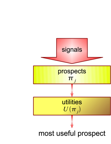
Figure 1: Scheme of the deterministic decision making process based on the choice of the most useful prospect with the largest expected utility.

The central aim of expected utility theory is to calculate the expected utilities for all prospects from the given family $\mathcal{L}$ and, comparing their values, to find the prospect possessing the largest utility. Then the decision is taken by selecting this prospect corresponding to the largest utility, which is called the most useful prospect. The decision making scheme based on expected utility theory is given in Fig. 1.

3 Probabilistic approach to expected utility theory

According to the expected utility theory delineated above, the choice of a prospect is with certainty prescribed by the utility of the prospects. This theory is deterministic, since the choice, with probability one, is required to correspond to the prospect with the largest expected utility. Such a completely deterministic formulation contradicts the known empirical facts demonstrating that, under the same conditions, different persons often choose different prospects. Of course, one could salvage the deterministic theory by introducing heterogenous utility functions that describe the variety of tastes of different people [28]. While this captures the evident observation that tastes exhibit some heterogeneity, extending utility theory to heterogeneous or random utility theory comes at the cost of a proliferation of parameters, making the approach descriptive at best, while being non-parsimonious and non predictive. An even more convincing attack to the deterministic approach comes from the observation that the same person, under the same conditions, may choose different prospects at different times. This “intra-observer variation” has been largely documented in the medical literature [29, 30]. This suggests to view the brain of a decision maker as deliberating on the set of admissible prospects and evaluating them by involving some probabilistic weighting. This is the motivation to reformulate utility theory by generalizing it to a probabilistic approach.

The probabilistic weighting of prospects can be formalized by invoking the principle of minimal information that allows one to find a probability distribution under the minimal given information. The idea of this principle goes back to Gibbs [31, 32, 33], who formulated it as a conditional maximization of entropy under the given set of constraints. This principle is widely used in information science [34] and in physics [35, 36]. A general convenient form of an information functional is given by the Kullback-Leibler relative information [37, 38].

In order to weight the prospects according to their utility, let us consider a family of prospects $\mathcal{L}$. Assume that they can be weighted by means of a distribution defined by utility factors $f(\pi_{j})$ that are normalized,

$$\sum_{j=1}^{L}f(\pi_{j})=1\;,\qquad 0\leq f(\pi_{j})\leq 1\;.$$ (8)

By definition, the utility factor of zero utility is to be zero,

$$f(\pi_{j})=0\;,\qquad U(\pi_{j})=0\;.$$ (9)

Since the utility factors $f(\pi_{j})$ weight the finite utilities $U(\pi_{j})$, the total finite expected utility defined by

$$U=\sum_{j=1}^{L}U(\pi_{j})f(\pi_{j})\;$$ (10)

should exist, given a finite number $L$ of prospects.

Under these conditions, we can define the Kullback-Leibler information as

$$I[f]=\sum_{j}f(\pi_{j})\ln\;\frac{f(\pi_{j})}{f_{0}(\pi_{j})}\;+\;\lambda\left[\sum_{j}f(\pi_{j})-1\right]\;-\;\beta\left[\sum_{j}U(\pi_{j})f(\pi_{j})-U\right]\;,$$ (11)

with a trial distribution $f_{0}(\pi_{j})$ proportional to the expected utility $U(\pi_{j})$ in order to take into account condition (9). The parameters $\lambda$ and $\beta$ are the Lagrange multipliers guaranteeing the validity of the imposed constraints (normalization (8) and existence of a well-defined finite expected utility (10)) .

Minimizing the information functional (11) yields the utility factor

$$f(\pi_{j})=\frac{U(\pi_{j})}{Z}\;\exp\{\beta U(\pi_{j})\}\;,$$ (12)

with a normalization coefficient

$$Z=\sum_{j}U(\pi_{j})\exp\{\beta U(\pi_{j})\}\;.$$

The parameter $\beta$ characterizes the level of belief or confidence of the decision maker in the correct selection of the prospect set. Requiring that the utility factor, by its definition, be an increasing function of utility makes the belief parameter non-negative $(\beta\geq 0)$.

In the case of no confidence in the given set of prospects, we have

$$f(\pi_{j})=\frac{U(\pi_{j})}{\sum_{j}U(\pi_{j})}\qquad(\beta=0)\;.$$ (13)

In the opposite case of absolute confidence, we get

$$f(\pi_{j})=\left\{\begin{array}[]{ll}1,&~{}~{}\pi_{j}=\max_{j}\pi_{j}\\ 0,&~{}~{}\pi_{j}<\max_{j}\pi_{j}\end{array}\right.\qquad(\beta\rightarrow\infty)\;,$$ (16)

where $\max_{j}\pi_{j}$ is the prospect whose expected utility is the largest. Thus, the latter situation $(\beta\rightarrow\infty)$ retrieves the deterministic utility theory, which hence can be seen as a particular case of the more general probabilistic approach.

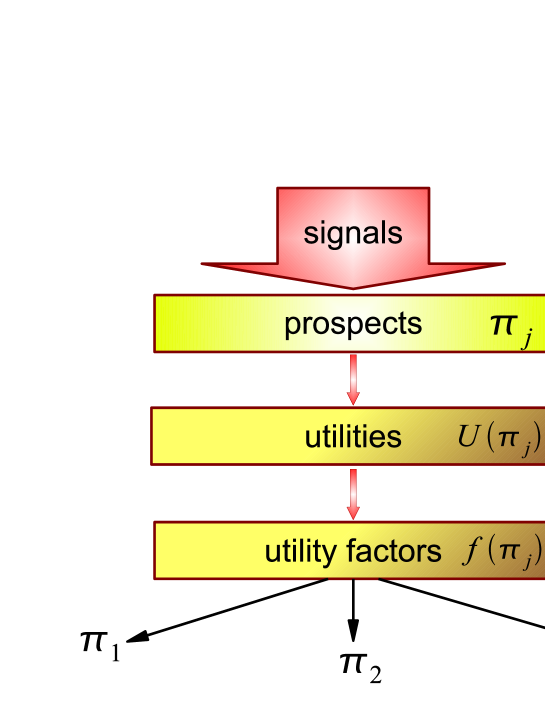
Figure 2: Scheme of the probabilistic decision making process based on the evaluation of the prospect utility factors characterizing the fraction of decision makers choosing the related prospect.

The prospect utility factors $\{f(\pi_{j}):j=1,2,...,L\}$ give the fractions of decision makers selecting the corresponding prospects $\{\pi_{j}:j=1,2,...,L\}$. The ordering of prospects in the probabilistic approach is the same as in the standard expected utility theory. But now, not all subjects are forced to choose the most useful prospect, though it is the prospect whose choice is the most probable. There can exist a fraction of decision makers choosing other prospects with lower utility. The probabilistic decision making scheme is summarized in Fig. 2.

4 Human decision making and computer operations

It is widely believed that the human brain operates, during a decision making process, as a complex and powerful computer. The network of neurons within the brain accepts external signals and transforms them into decisions of the subject by accomplishing the corresponding actions [39]. Such a procedure could correspond to the schemes depicted in Fig. 1 or Fig. 2.

However, if the brain would act as just described, this would correspond to making decisions only on the basis of a well defined deterministic objective function, called utility. But there exist numerous empirical studies demonstrating that humans often deviate from and even contradict the choices prescribed by utility theory. Such contradictions are known as decision-making paradoxes. As examples, we can mention the Allais paradox [40], the Ellsberg paradox [41], the Kahneman-Tversky paradox [42], the Rabin paradox [43], the Ariely paradox [44], the disjunction effect [45], the conjunction fallacy [46], the planning paradox [47], and many others [48, 49]. These paradoxes cannot be resolved by the approaches consisting in modifying the expected utility theory into so-called non-expected utility theories, as has been proved in Refs. [50, 51].

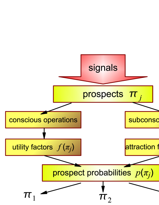
Figure 3: Scheme of human decision making, which is at the basis of the Quantum Decision Theory proposed here.

The appearance of numerous paradoxes in decision making, based on utility theory, is caused by the fact that this theory does not take into account the emotional components always present in decision makers, which often compete and modify the decisions that would result purely from utility-based processes. A human decision maker not merely evaluates the objective utility of the prospects, but also is influenced by subjective feelings, emotions, and behavioral biases that are produced by subconscious brain activity. The brain takes decisions by combining (i) the objective knowledge of the prospect utility, by evaluating the utility factors, with (ii) the subjective attractiveness of the prospects, which is hinted by subconscious feelings. The latter means that, in addition to the utility factors measured by conscious logical operations, there should exist attraction factors produced by subconscious feelings. Then, the resulting weights of the prospects $p(\pi_{j})$ are defined not merely by the utility factors $f(\pi_{j})$, but are also dependent on some attraction factors $q(\pi_{j})$. We thus suggest that the correct representation of the brain function during a decision process is given by the scheme represented in Fig. 3, which should correct and replace those of Figs. 1 or 2.

Our theory views the human brain not just a powerful computer accomplishing a great number of straightforward logical operations, but as an object that must include parallel functioning on two levels. One part, representing conscious logical operations evaluating the utility factors, can be organized as a powerful computer. And the other part, representing subconscious activity producing the attraction factors, should be a very different device that functions not as a straightforward computer calculating numbers, but as an object estimating qualitative features of the prospects.

In the sequel, we do not touch on the technical issues of how the devices, discussed above, are actually structurally realized, or how they could be constructed in an artificial brain. Instead, we describe how their functioning can be represented mathematically, characterizing the split dual action of evaluating the prospect utilities and estimating their attractiveness.

5 Quantum decision making by human brain

The dualism of the brain, combining objective conscious operations with subjective subconscious activity, suggests that its functions could be described by generalizing the real-valued way of defining the prospect weights to an approach involving complex-valued quantities. In turn, this immediately points to quantum-theory techniques, where the probability weights are defined through complex-valued quantities, such as wave functions.

The idea of employing quantum theory for describing brain functions was advanced by Bohr [52, 53]. Analyzing the quantum theory of measurements, von Neumann [54] mentioned that the action of measuring observables could be interpreted, to some extent, as taking decisions. Using these ideas, we have developed [16, 17, 18, 19, 20, 21] the Quantum Decision Theory (QDT), using the mathematical techniques of quantum theory of measurements.

Before formulating this theory, we would like to stress that the quantum approach to describing human decision making does not assume that the brain is a quantum object. The quantum techniques just provide the most straightforward way of generalizing decision making by taking into account the dual functioning of the human brain.

The main points of QDT are as follows. We consider a set of elementary prospects, represented by vectors $|n\rangle$, whose closed linear envelope

$${\cal H}\equiv{\rm Span}\{|n\rangle\}$$ (17)

composes the space of mind. The prospects $\pi_{j}$ from the given set $\mathcal{L}$ are represented by the vectors $|\pi_{j}\rangle$ in the space of mind. The prospect operators are defined as

$$\hat{P}(\pi_{j})\equiv|\pi_{j}\rangle\langle\pi_{j}|\;.$$ (18)

These operators play the same role as the operators from the algebra of local observables in quantum theory.

The state of a decision maker is characterized by a non-negative operator $\rho$ acting on the space of mind and normalized as

$${\rm Tr}\hat{\rho}=1\;,$$

with the trace taken over the space of mind. Defining the decision-maker state by a statistical operator, but not by a simple wave function, takes into account that this decision maker is not an absolutely isolated subject, but can be influenced by its environment.

The prospect probabilities, playing the role of observable quantities, are defined as the averages of the prospect operators

$$p(\pi_{j})\equiv{\rm Tr}\hat{\rho}\hat{P}(\pi_{j})\;,$$ (19)

with the trace again taken over the space of mind. Writing down the explicit expression for the trace over the elementary prospect states and separating the diagonal and off-diagonal parts leads to the sum

$$p(\pi_{j})=f(\pi_{j})+q(\pi_{j})\;,$$ (20)

in which the first term comes from the diagonal part and the second term, from the off-diagonal part. The first term represents the classical utility factor, while the second term, caused by the prospect quantum interference, is the attraction factor. By definition, the prospect probability is non-negative and normalized, so that

$$\sum_{j=1}^{L}p(\pi_{j})=1\;\qquad 0\leq p(\pi_{j})\leq 1\;.$$ (21)

In view of the normalization condition for the utility factor (8), the attraction factor lies in the range

$$-1\leq q(\pi_{j})\leq 1$$ (22)

and satisfies the alternation law

$$\sum_{j=1}^{L}q(\pi_{j})=0\;.$$ (23)

Generally, the attraction factor is a contextual quantity that can vary for different decision makers and even for the same decision maker at different times. This looks as an obstacle for the ability to give quantitative predictions for the prospect probabilities. However, it is possible to show [18, 21] that the aggregate attraction factor, averaged over many decision makers, enjoys the property called quarter law:

$$\frac{1}{L}\;\sum_{j=1}^{L}|q(\pi_{j})|=\frac{1}{4}\;.$$ (24)

Since the utility factor is uniquely defined by the corresponding expected utility, it is possible to estimate quantitatively the prospect probabilities, assuming that the typical attraction factor satisfies the quarter law.

When the decision maker is a member of a society from which he/she gets additional information, then the attraction factor varies depending on the amount $\mu$ of the received information. The attraction factor, as a function of the information measure $\mu$, can be presented [55] in the form

$$q(\pi_{j},\mu)=q(\pi_{j},0)e^{-\gamma\mu}\;.$$ (25)

The information can be positive, with $\mu>0$ as well as negative, or misleading, with $\mu<0$. Respectively, the attraction factor can either decrease or increase. The attenuation of behavioral biases with the receipt of additional information has been confirmed by empirical studies [56, 57].

The reduction of QDT to the probabilistic variant of classical decision theory corresponds to the attraction factor tending to zero. This is similar to the reduction of quantum theory to classical statistical theory in the process of decoherence.

6 Cooperation paradox in prisoner dilemma games

Let us briefly summarize the status of QDT with respect to its empirical support. First, the disjunction effect, studied in different forms in a variety of experiments [45], has been analyzed in details in [18, 21], where we found that the empirically determined absolute value of the aggregate attraction factor $|q(\pi_{j})|$ was found to coincide with the value $0.25$ predicted by expression (24), within the typical statistical error of the order of $20\%$ characterizing these experiments. The same agreement, between the QDT prediction for the absolute value of the attraction factors and empirical values, holds for experiments testing the conjunction fallacy. The planning paradox has also found a natural explanation within QDT [17]. Moreover, it has been shown [20] that QDT explains practically all typical paradoxes of classical decision making, arising when decisions are taken by separate individuals.

In order to illustrate how QDT resolves classical paradoxes, let us consider a typical paradox happening in decision making. In game theory, there is a series of games, in which several subjects can choose either to cooperate with each other or to defect. Such setups have the general name of prisoner dilemma games. The cooperation paradox consists in the real behavior of game participants who often incline to cooperate despite the prescription of utility theory for defection. Below, we show that this paradox is easily resolved within QDT, which gives correct quantitative predictions.

The generic structure of the prisoner dilemma game is as follows. Two participants can either cooperate with each other or defect from cooperation. Let the cooperation action of one of them be denoted by $C_{1}$ and the defection by $D_{1}$. Similarly, the cooperation of the second subject is denoted by $C_{2}$ and the defection by $D_{2}$. Depending on their actions, the participants receive payoffs from the set

$$\mathbb{X}=\{x_{1},x_{2},x_{3},x_{4}\}\;,$$ (26)

whose values are arranged according to the inequality

$$x_{3}>x_{1}>x_{4}>x_{2}\;.$$ (27)

There are four admissible cases: both participants cooperate $(C_{1}C_{2})$, one cooperates and another defects $(C_{1}D_{2})$, the first defects but the second cooperates $(D_{1}C_{2})$, and both defect $(D_{1}D_{2})$. The payoffs to each of them, depending on their actions, are given according to the rule

$$\left[\begin{array}[]{cc}C_{1}C_{2}&C_{1}D_{2}\\ D_{1}C_{2}&D_{1}D_{2}\end{array}\right]\rightarrow\left[\begin{array}[]{cc}x_{1}x_{1}&x_{2}x_{3}\\ x_{3}x_{2}&x_{4}x_{4}\end{array}\right]\;.$$ (32)

As is clear, the enumeration of the participants is arbitrary, so that it is possible to analyze the actions of any of them.

Each subject has to decide what to do, to cooperate or to defect, when he/she is not aware about the choice of the opponent. Then, for each of the participants, there are two prospects, either to cooperate,

$$\pi_{1}=C_{1}(C_{2}+D_{2})\;,$$ (33)

or to defect,

$$\pi_{2}=D_{1}(C_{2}+D_{2})\;.$$ (34)

In the absence of any information on the action chosen by the opponent, the probability for each of these actions is $1/2$ (non-informative prior). Assuming for simplicity the linear utility as a utility function of the payoffs, the expected utility of cooperation for the first subject is

$$U(\pi_{1})=\frac{1}{2}\;x_{1}+\frac{1}{2}\;x_{2}\;,$$ (35)

while the utility of defection is

$$U(\pi_{2})=\frac{1}{2}\;x_{3}+\frac{1}{2}\;x_{4}\;.$$ (36)

The assumption of linear utility is not crucial, and can be removed by reinterpreting the payoff set (26) as the utility set. Because of condition (27), the utility of defection is always larger than that of cooperation, $U(\pi_{2})>U(\pi_{1})$. According to utility theory, this means that all subjects have always to prefer defection.

However, numerous empirical studies demonstrate that an essential fraction of participants choose to cooperate despite the prescription of utility theory. This contradiction between reality and the theoretical prescription constitutes the cooperation paradox [58, 59].

Considering the same game within the framework of QDT, we have the probabilities of the two prospects,

$$p(\pi_{1})=f(\pi_{1})+q(\pi_{1})\;,\qquad p(\pi_{2})=f(\pi_{2})+q(\pi_{2})\;.$$ (37)

The propensity to cooperation and the presumption of innocence propose that the attraction factor for cooperative prospect is larger than that for the defecting prospect, that is, $q(\pi_{1})>q(\pi_{2})$. In view of the alternation law (23) and quarter law (24), we have

$$q(\pi_{1})=-q(\pi_{2})=\frac{1}{4}\;.$$ (38)

Hence, we can estimate the considered prospects by the equations

$$p(\pi_{1})=f(\pi_{1})+0.25\;,\qquad p(\pi_{2})=f(\pi_{2})-0.25\;.$$ (39)

From here, we see that, even if defection seems to be more useful than cooperation, so that $f(\pi_{2})>f(\pi_{1})$, the cooperative prospect can be preferred by some of the participants.

To illustrate numerically how this paradox is resolved, let us take the data from the experimental realization of the prisoner dilemma game by Tversky and Shafir [45]. Subjects played a series of prisoner dilemma games, without feedback. Three types of setups were used: (i) when the subjects knew that the opponent had defected, (ii) when they knew that the opponent had cooperated, and (iii) when subjects did not know whether their opponent had cooperated or defected. The rate of cooperation was $3\%$ when subjects knew that the opponent had defected, and $16\%$ when they knew that the opponent had cooperated. However, when subjects did not know whether their opponent had cooperated or defected, the rate of cooperation was $37\%$.

Treating the utility factors as classical probabilities, we have

$$f(\pi_{1})=\frac{1}{2}\;f(C_{1}|C_{2})+\frac{1}{2}\;f(C_{1}|D_{2})\;,$$

$$f(\pi_{2})=\frac{1}{2}\;f(D_{1}|C_{2})+\frac{1}{2}\;f(D_{1}|D_{2})\;.$$

According to the Tversky-Shafir data,

$$f(C_{1}|C_{2})=0.16\;,\qquad f(C_{1}|D_{2})=0.03\;.$$

Hence,

$$f(\pi_{1})=0.095\;,\qquad f(\pi_{2})=0.905\;.$$ (40)

Then, for the prospect probabilities (39), we get

$$p(\pi_{1})=0.345\;,\qquad p(\pi_{2})=0.655\;.$$ (41)

In this way, the fraction of subjects choosing cooperation is predicted to be about $35\%$. This is in remarkable agreement with the empirical data of $37\%$ by Tversky and Shafir. Actually, within the statistical accuracy of the experiment, the predicted and empirical numbers are indistinguishable.

If we would follow the classical approach, the fraction of cooperators should be not larger than $10\%$ ($f(\pi_{1})$), which is much smaller than the observed $37\%$. But in QDT, there are no paradoxes and its predictions are in quantitative agreement with empirical observations.

7 Conclusion

We have presented the Quantum Decision Theory that we have developed in the last four years, which is based on combining utility-like calculations with emotional influences in the representation of the decision making processes. We have emphasized that decision making by humans is principally different from the direct calculations by, even the most powerful, computers. This basic difference is in the duality of the human decision-making procedure. The brain makes decisions by a parallel processing of two different jobs: by consciously estimating the utility of the available prospects and by subconsciously evaluating their attractiveness.

We have shown how the duality of the brain functioning can be adequately represented by the techniques of quantum theory. The process of decision making has been described as mathematically similar to the procedure of quantum measurement. The self-consistent mathematical theory of human decision making that we have been developed contains no paradoxes typical of classical decision making. It is important to stress that this theory is the first theory allowing for it quantitative predictions taking into account behavioral biases.

We stress that the description of the functioning of the human brain by means of quantum techniques does not require that the brain be a quantum object, but this approach serves as an appropriate mathematical tool for characterizing the conscious-subconscious duality of the brain processes. This duality must be taken into account when one attempts to create an artificial intelligence imitating the human brain. Such an artificial intelligence has to be quantum in the sense explained above [60].

Acknowledgment

The authors are grateful for many discussions with and advice from M. Favre and E.P. Yukalova. Financial support form the Swiss National Science Foundation is appreciated.

Figure captions

Fig. 1. Scheme of the deterministic decision making process based on the choice of the most useful prospect with the largest expected utility.

Fig. 2. Scheme of the probabilistic decision making process based on the evaluation of the prospect utility factors characterizing the fraction of decision makers choosing the related prospect.

Fig. 3. Scheme of human decision making, which is at the basis of the Quantum Decision Theory proposed here.

References

- [1] F.A.C. Azevedo, L.R.B. Carvalho, L.T. Grinberg, J.M. Farfel, R.E.L. Ferretti, R.E.P. Leite, W.J. Filho, R. Lent and S. Herculano-Houzel, Equal numbers of neuronal and non-neuronal cells make the human brain an isometrically scaled-up primate brain. J. Compar. Neurol. 513, 532–541 (2009).
- [2] G.M. Shepherd, Neurobiology (Oxford University, Oxford, 1994).
- [3] E.R. Kandel, J.H. Schwartz, and T.M. Jessel, Principles of Neural Science (McGraw-Hill, New York, 2000).
- [4] O. Sporns, Networks of the Brain (Massachusetts Institute of Technology, New York, 2011).
- [5] A.R. Luria, Higher Cortical Functions in Man (Basic Books, New York, 1966).
- [6] D. Elkind and J. Flavell, Studies in Cognitive Development (Oxford University, New York, 1969).
- [7] R.J. Sternberg and W. Salter, Handbook of Human Intelligence (Cambridge University, Cambridge, 1982).
- [8] J.P. Das, J.A. Naglieri, and J.R. Kirby, Assessment of Cognitive Processes (Allyn and Bacon, Needham Heights, 1994).
- [9] W.K. Wake, H. Gardner, and M.L. Kornhaber, Intelligence: Multiple Perspectives (Harcourt Brace College, Fort Worth, 1996).
- [10] K. Richardson, The Making of Intelligence (Columbia University, New York, 2000).
- [11] R.J. Sternberg, ed. International Handbook of Intelligence (Cambridge University, Cambridge, 2004).
- [12] K. Stanovich, What Intelligence Tests Miss: The Psychology of Rational Thought (Yale University, New Haven, 2009).
- [13] S. Coren, The Intelligence of Dogs (Bantam Books, New York, 1995).
- [14] A. Trewavas, Green plants as intelligent organisms. Trends Plant Sci. 10, 413–419 (2005).
- [15] J. Canny, S.J. Russell, and P. Norvig, Artificial Intelligence: A Modern Approach (Prentice Hall, Englewood Cliffs, 2003).
- [16] V.I. Yukalov and D. Sornette, Quantum decision theory as quantum theory of measurement. Phys. Lett. A 372, 6867–6871 (2008).
- [17] V.I. Yukalov and D. Sornette, Physics of risk and uncertainty in quantum decision making. Eur. Phys. J. B 71, 533–548 (2009).
- [18] V.I. Yukalov and D. Sornette, Processing information in quantum decision theory. Entropy 11, 1073–1120 (2009).
- [19] V.I. Yukalov and D. Sornette, Entanglement production in quantum decision making. Phys. At. Nucl. 73, 559–562 (2010).
- [20] V.I. Yukalov and D. Sornette, Mathematical structure of quantum decision theory. Adv. Complex Syst. 13, 659–698 (2010).
- [21] V.I. Yukalov and D. Sornette, Decision theory with prospect interference and entanglement. Theor. Dec. 70, 283–328 (2011).
- [22] J. von Neumann and O. Morgenstern, Theory of Games and Economic Behavior (Princeton University, Princeton, 1953).
- [23] L.J. Savage, The Foundations of Statistics (Wiley, New York, 1954).
- [24] J.W. Pratt, Risk aversion in the small and in the large. Econometrica 32, 122–136 (1964).
- [25] K.J. Arrow, Essays in the Theory of Risk Bearing (Markham, Chicago, 1971).
- [26] D. Graeber, Debt: The First 5,000 Years (Melville House, New York, 2011).
- [27] D. Bernoulli, Exposition of a new theory on the measurement of risk. Proc. Imper. Acad. Sci. St. Petersburg 5, 175–192 (1738).
- [28] D. McFadden, Econometric models of probabilistic choice. In Structural Analysis of Discrete Data with Econometric Applications, C.F. Manski and D. McFadden (eds.) (Massachusetts Institute of Technology, Cambridge, 1981), p. 198–272.
- [29] I.M. Rutkow, Surgical decision making, the reproducibility of clinical judgment. Arch. Surg. 117, 337–340 (1982).
- [30] J.O. Nielsen, H. Dons-Jensen, and H.T. Sarrensen, Lauge-Hansen classification of malleolar fractures, an assessment of the reproducibility in 118 cases. Acra Orthop. Scand. 61, 385–387 (1990).
- [31] J.W. Gibbs, Elementary Principles in Statistical Mechanics (Oxford University, Oxford, 1902).
- [32] J.W. Gibbs, Collected Works (Longmans, New York, 1928) Vol. 1.
- [33] J.W. Gibbs, Collected Works (Longmans, New York, 1931) Vol. 2.
- [34] C.E. Shannon and W. Weaver, Mathematical Theory of Communication (University of Illinois, Urban, 1949).
- [35] E.T. Jaynes, Information theory and statistical mechanics. Phys. Rev. 106, 620–630 (1957).
- [36] V.I. Yukalov, Phase transitions and heterophase fluctuations. Phys. Rep. 208 395–492 (1991).
- [37] S. Kullback and R.A. Leibler, On information and sufficiency. Ann. Math. Stat. 22 79–86 (1951).
- [38] S. Kullback, Information Theory and Statistics (Wiley, New York, 1959).
- [39] K. Mainzer, Thinking in Complexity (Springer, Berlin, 2007).
- [40] M. Allais, Le comportement de l’homme rationnel devant le risque: critique des postulats et axiomes de l’ecole Americaine. Econometrica 21, 503–546 (1953).
- [41] D. Ellsberg, Risk, ambiguity, and the Savage axioms. Quart. J. Econ. 75, 643–669 (1961).
- [42] D. Kahneman and A. Tversky, Prospect theory: an analysis of decision under risk. Econometrica 47, 263–291 (1979).
- [43] M. Rabin, Risk aversion and expected-utility theory: a calibration theorem. Econometrica 68, 1281–1292 (2000).
- [44] D. Ariely, Predictably Irrational (Harper, New York, 2008).
- [45] A. Tversky and E. Shafir, The disjunction effect in choice under uncertainty. Psychol. Sci. 3, 305–309 (1992).
- [46] A. Tversky and D. Kahneman, Extensional versus intuitive reasoning: the conjunction fallacy in probability judgement. Psychol. Rev. 90, 293–315 (1983).
- [47] F.E. Kydland and E.C. Prescott, Rules rather than discretion: the inconsistency of optimal plans. J. Polit. Econ. 85, 473–492 (1977).
- [48] C.F. Camerer, G. Loewenstein, and R. Rabin, eds., Advances in Behavioral Economics (Princeton University, Princeton, 2003).
- [49] M.J. Machina, Non-expected utility theory. In: New Palgrave Dictionary of Economics. S.N. Durlauf and L.E. Blume, eds., (Macmillan, New York, 2008).
- [50] Z. Safra and U. Segal, Calibration results for non-expected utility theories. Econometrica 76, 1143–1166 (2008).
- [51] N.I. Al-Najjar and J. Weinstein, The ambiguity aversion literature: a critical assessment. Econ. Philos. 25, 249–284 (2009).
- [52] N. Bohr, Light and life. Nature 131, 421–423, 457–459 (1933).
- [53] N. Bohr, Atomic Physics and Human Knowledge (Wiley, New York, 1958).
- [54] J. von Neumann, Mathematical Foundations of Quantum Mechanics (Princeton University, Princeton, 1955).
- [55] V.I. Yukalov and D. Sornette, Theory of behavioral decision biases of social agents, http://ssrn.com/abstract=2018270 (2012).
- [56] A. Kühberger, D. Komunska, and J. Perner, The disjunction effect: does it exist for two-step gambles? Org. Behav. Human Decis. Proc. 85, 250–264 (2001).
- [57] G. Charness, E. Karni, and D. Levin, On the conjunction fallacy in probability judgement: new experimental evidence regarding Linda. Games Econ. Behav. 68, 551–556 (2010).
- [58] C. Camerer, Behavioral Game Theory (Princeton University, Princeton, 2003).
- [59] A. Tversky, Preference, Belief, and Similarity: Selected Writings (Massachusetts Institute of Technology, Cambrideg, 2004).
- [60] V.I. Yukalov and D. Sornette, Scheme of thinking quantum systems. Laser Phys. Lett. 6, 833–839 (2009).