Dust properties inside molecular clouds from coreshine modeling and observations

Abstract

Context. Using observations to deduce dust properties, grain size distribution, and physical conditions in molecular clouds is a highly degenerate problem.

Aims. The coreshine phenomenon, a scattering process at 3.6 and 4.5 $\mu$m that dominates absorption, has revealed its ability to explore the densest parts of clouds. We want to use this effect to constrain the dust parameters. The goal is to investigate to what extent grain growth (at constant dust mass) inside molecular clouds is able to explain the coreshine observations. We aim to find dust models that can explain a sample of Spitzer coreshine data. We also look at the consistency with near-infrared data we obtained for a few clouds.

Methods. We selected four regions with a very high occurrence of coreshine cases: Taurus–Perseus, Cepheus, Chameleon and L183/L134. We built a grid of dust models and investigated the key parameters to reproduce the general trend of surface brightnesses and intensity ratios of both coreshine and near-infrared observations with the help of a 3D Monte-Carlo radiative transfer code. The grid parameters allow to investigate the effect of coagulation upon spherical grains up to 5 $\mu$m in size derived from the DustEm diffuse interstellar medium grains. Fluffiness (porosity or fractal degree), ices, and a handful of classical grain size distributions were also tested. We used the near– and mostly mid–infrared intensity ratios as strong discriminants between dust models.

Results. The determination of the background field intensity at each wavelength is a key issue. In particular, an especially strong background field explains why we do not see coreshine in the Galactic plane at 3.6 and 4.5 $\mu$m. For starless cores, where detected, the observed 4.5 $\mu$m / 3.6 $\mu$m coreshine intensity ratio is always lower than $\sim$0.5 which is also what we find in the models for the Taurus–Perseus and L183 directions. Embedded sources can lead to higher fluxes (up to four times greater than the strongest starless core fluxes) and higher coreshine ratios (from 0.5 to 1.1 in our selected sample).
Normal interstellar radiation field conditions are sufficient to find suitable grain models at all wavelengths for starless cores. The standard interstellar grains are not able to reproduce observations and, due to the multi-wavelength approach, only a few grain types meet the criteria set by the data. Porosity does not affect the flux ratios while the fractal dimension helps to explain coreshine ratios but does not seem able to reproduce near–infrared observations without a mix of other grain types.

Conclusions. Combined near– and mid–infrared wavelengths confirm the potential to reveal the nature and size distribution of dust grains. Careful assessment of the environmental parameters (interstellar and background fields, embedded or nearby reddened sources) is required to validate this new diagnostic.

1 Introduction

The study of low mass star and of planet formation starts by understanding the place where they form and evolve, that is inside dense molecular clouds. There, the gas and the dust are in constant interaction through collisions that can lead to heat exchange and, in suitable conditions, to the freezing of gas molecules onto dust grains. Inside the molecular cloud, the dust content is known to evolve mainly via grain growth: by accretion of heavy gas particles on the dust grains that increases the total dust mass (Hirashita 2012), and by the presence of sticky ice mantles (volatile species frozen onto the grains, Walmsley et al. 2004) which favors coagulation (Ossenkopf 1993; Ormel et al. 2009). Ice mantle formation beyond A${}_{\mathrm{v}}\sim\,$3 mag (Whittet et al. 2001, 2013) implies a change in the grain properties throughout molecular clouds. In addition, interstellar grains evolve with time during the prestellar phase. They continue to grow or possibly reach a stationary state in the cloud envelope (Ormel et al. 2009) while, in the densest region, the dust evolution becomes complex in the presence of an embedded object such as Class 0 or Class I protostars (André et al. 2000). The thermo-mechanical action of the protostellar object will affect the grains by shattering them in the outflows (Anderl et al. 2013) and by evaporating the grain mantles, releasing water (and other species) in the surrounding gas (Fraser et al. 2001), as seen by Herschel (Kristensen et al. 2012; van der Tak et al. 2013). In this context, to infer the molecular cloud stage from the dust properties is a complex problem which starts by understanding the dust grain content.

Grain properties can be investigated in different manners, for example via the characterization of the extinction curve. In the optical and UV, this curve changes depending on the dominant grain growth mechanism: accretion or coagulation (Hirashita & Voshchinnikov 2014). In the near-infrared (NIR) and mid-infrared (MIR) ranges, this change is a clue to coagulation (Chapman et al. 2009; Ascenso et al. 2012) and to the presence of ice mantles (McClure 2009). Nevertheless, grain growth deduced indirectly from the extinction curve is sensitive to the wavelength normalization (Fitzpatrick & Massa 2007). In this context, a very efficent way to learn about the properties of larger grains (micrometer size) is through the recently discovered effect of MIR dust scattering or ”coreshine effect” (Pagani et al. 2010; Steinacker et al. 2010). The coreshine effect is widespread and detected in at least half of the molecular clouds investigated by Pagani et al. (2010) and Paladini et al. (in prep.), and thus can be used as a tool to explore the properties of the dust responsible for such a phenomenon.

Coreshine is observed at those MIR wavelengths, 3–5 $\mu$m, where the scattering by large grains is strong enough to be seen in emission. The best examples are seen in the 3.6 and 4.5 $\mu$m Spitzer Infrared Array Camera (IRAC) filters (Pagani et al. 2010). When the absence of emission in the 5.8 and 8 $\mu$m IRAC filters excludes the presence of Polycyclic Aromatic Hydrocarbons (PAHs), there is no need to consider an active emission process in the modeling and only scattering and absorption have to be treated, as presented in Steinacker et al. (2010). The same restriction to absorption and scattering modeling is also pertinent for shorter wavelengths (optical and NIR) as demonstrated by Lehtinen & Mattila (1996) for a standard InterStellar Radiation Field (ISRF).

The investigation potential of coreshine, combined with the modeling of other wavelengths provides an opportunity to better constrain both cloud structures and dust properties. Indeed, thanks to the low opacities at MIR wavelengths and to the anisotropic scattering, coreshine provides access deep inside the clouds and brings information on their 3D structure. The feasibility of the method has been shown (Steinacker et al. 2010; Andersen et al. 2013) but to quantify our capacity to build a 3D model of a real cloud and deduce grain properties from a combination of wavelengths, we need to evaluate the impact of the free parameters and of the boundary conditions on the modeling. Here, we compare our models to observations and deduce general trends on the grain properties for the regions where most of the clouds present coreshine. The set of dust models will constitute a future data base to start modeling molecular clouds in absorption and scattering from visible to MIR. In a forthcoming paper, we will model a specific cloud while also including the far–infrared (FIR) emission to further constrain the dust properties and cloud structure.

In Sect. 2, we present a summary of the observations and the strategy adopted to analyze them. In Sect. 3, we describe the Monte Carlo radiative transfer code used for the simulations, focus on the importance of constraining the radiation field and present the cloud model and the dust content which are the free parameters to be explored. In Sect. 4, we describe the results obtained from the observational data and confront them with our grid of models. We discuss the coreshine phenomenon and what a multi-wavelength approach can bring to investigate the grain properties. We present our conclusions in Sect. 5.

2 Observations and Analysis

2.1 NIR data

NIR data have been obtained with WIRCAM, the CFHT Wide IR CAMera. Its field of view is 20′$\times$20′ with a pixel size of 0.3″. It is large enough to cover each of the selected targets including a large area around them. The observations were obtained (and continue currently to be taken) for a total of eight sources (L183 and a set of sources in the Taurus region) in the standard J, H, and Ks (hereafter K) spectral bands. The observations, data processing and data themselves will be presented in detail in a forthcoming paper. We use some J and K band observations to have a first look at the comparison with models, without performing any exact fits.

2.2 Coreshine data

To investigate the presence of coreshine phenomenon inside a sample of molecular clouds, we used Spitzer data taken by IRAC (Fazio et al. 2004) at 3.6, 4.5, 5.8 and 8 $\mu$m (Cryogenic mission) complemented by that from the Warm mission (3.6 and 4.5 $\mu$m only). When possible, the 3.6 and 4.5 $\mu$m data have been compared to Spitzer 8 $\mu$m and/or WISE 12 $\mu$m  maps (Wright et al. 2010) to define the size of the core in absorption and optical data (in R or B) to delimit the size of the surrounding cloud. These Spitzer observations were collected at different epochs and show a median frame integration time per pixel from 50 seconds (From molecular cores to Planet forming disks (c2d) – Evans et al. 2009) to 1800 seconds (Hunting Coreshine Survey HCS, Spitzer cycles 8 and 9 – Paladini et al. in prep.). The sensitivity for a unit exposure time in the warm mode (HCS) is comparable to the one in the cold mode (P94 program: Search for Low-Luminosity YSOs - Lawrence & Keene 2004, c2d), which allows us to merge the observations. The aim of the HCS proposal was to obtain an unbiased sample, and our analysis confirms the $\sim$50% detection rate of coreshine as in Pagani et al. (2010, Paladini et al. in prep.).

The coverage is entirely dependent on the program and on the target. The Spitzer field of view size is 5.12′ $\times$ 5.12′ with a native pixel size of 1.2″. The Full Width Half Maximum (FWHM) of the Point Spread Function (PSF) varies from 1.66″ at 3.6 $\mu$m to 1.98″ at 8 $\mu$m. For the nearby molecular clouds, the maps are large enough to include both the cores and their environment. The sensitivity for an extended source at 4.5 $\mu$m is about 90% of the 3.6 $\mu$m sensitivity for both warm and cold campaigns. However, the data must be corrected for column pulldown and zodiacal emission (Paladini et al., in prep.). It must be noted that even if Spitzer data are absolutely calibrated using point sources, the extended emission calibration can be as uncertain as 10%. Indeed, while the drift of the electronics zero level is small, the zodiacal light estimate remains slightly uncertain because of its time dependence and the spatial resolution of the model used to derive it. Though this is of no importance for differential measurements, such as the coreshine intensity defined as the net signal above the background, it becomes a problem for evaluating the absolute background intensity behind the clouds. Indeed, the observational value I_back,Sp can vary by a factor of two from one campaign to another as the uncertainty on the zodiacal light estimate is of the same order as the background value itself (and consequently cannot be used as a reference for I_back in the modeling, Sect. 3.2.2).

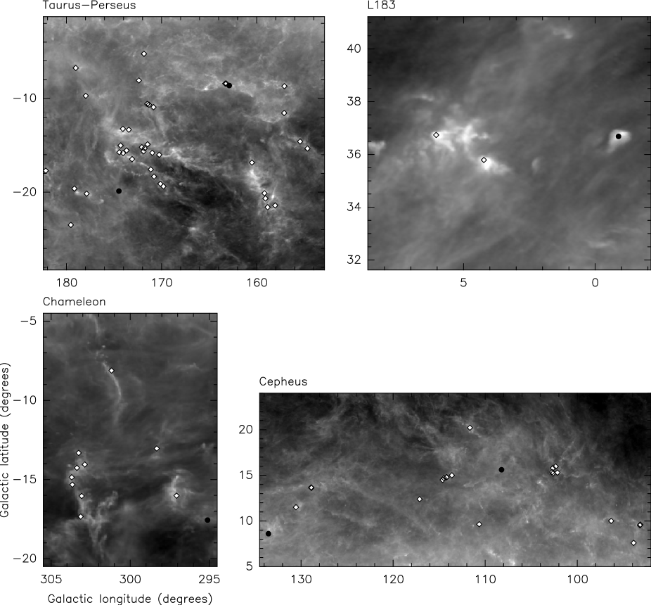
Figure 2: Zoom from Fig. LABEL:fig:planck on the four regions of interest.

The sample of the 215 sources presented in Table LABEL:tab:sources and in Fig. LABEL:fig:planck is essentially a compilation of previous surveys including c2d and P94 surveys which were the main archives for the identification of coreshine sources in Pagani et al. (2010), the new HCS survey (Paladini et al. in prep), plus a few more targets of interest detected thanks to WISE (Wright et al. 2010) or recently identified in the Spitzer Archive (including the Gum/Vela region, Pagani et al. 2012). The total number of clouds which show coreshine is 108 with some preferential directions on the sky. Indeed, the Taurus, Perseus, Aquila and Aries complex (hereafter Taurus–Perseus) reveals almost 100 % coreshine detection (Fig. 2, Table LABEL:tab:sources). Cepheus and Chameleon regions also display a large fraction of coreshine cases. Finally, because of its high galactic latitude and its complexity L183 will be also one of the regions of interest for this study. Among these 108 positive coreshine detections, we chose to ignore the cores located in Orion/Monoceros and $\rho$ Oph regions where the coreshine occurrence drops to $\sim$50% (Table LABEL:tab:sources). In these regions the coreshine occurrence is likely dominated by the effect of local sources which make the radiation field difficult to constrain, adding another degree of freedom. Therefore, they are beyond the goal of our global study of coreshine. After this selection criterium, we are left with 72 coreshine sources.

2.3 Analysis

From the observations, we want to quantify the scattering excess above the surrounding background. To proceed to the measurement two steps are mandatory: i) remove the point sources to keep only the extended emission, ii) subtract the background contribution (I_back,Sp) under the core to deduce the remaining intensity. For the present analysis, the SExtractor software (Bertin & Arnouts 1996) has been used and its parameters tuned in order to remove point sources and keep only the extended emission.

First, SExtractor computes the background from a large scale mesh. This coarse background is resampled to the original resolution, the fluctuations are dampened by applying a median filter to the mesh points. The result is subtracted internally from the original image. Next, the object detection step works on a smoothed image and requires to set up a detection threshold. The objects are detected from an image smoothed with a gaussian kernel that has a FWHM equal to 1.5 pixels. Each detection is required to contain at least 3 pixels above 1.5 $\sigma$. The difficulty here is to adjust the background mesh size so that the coreshine emission is removed as part of the background while the extended saturated stars remain in order to be detected as objects by SExtractor. If the mesh size is too small they will appear in the final image. On the other hand, if the mesh size is too large, the extended coreshine emission would not be included in the background estimate but detected instead as a source. The object identification file is checked and for most coreshine cases, we chose a mesh size of 32$\times$32 pixels, but sometimes we adapted the mesh size to 64$\times$64 instead. Then, the object list can be used to either remove the sources from the image for display or to produce a mask of the point sources for measurements. This source subtraction method with the optimized parameters works on almost all Spitzer maps (even in crowded fields) and allows us to mask or to subtract compact objects and to retrieve only extended emission (Fig. LABEL:fig:L183_sex).

Because coreshine is a phenomenon defined as a signal in excess with respect to the surrounding background emission, the coreshine intensity has to be background subtracted. To perform this subtraction, it is mandatory to interpolate the background value (I_back,Sp) at the core position. Due to the extended nature of the coreshine effect, the process cannot be automatized. After having subtracted the point sources, we mask the coreshine region by hand and subtract either a plane by least square fitting or repeat the background subtraction process with SExtractor, interpolating across the coreshine masked region. This interpolation is usually safe when the masked region remains small but can become less accurate for large sources. However, the interpolation of the background is normally close to a plane. We compared both subtraction methods for the very extended coreshine emission present in L183 and found good agreement between the two methods, with a difference smaller than 10%.

The 3.6 and 4.5 $\mu$m cleaned images are convolved with a gaussian kernel of 10″ FWHM to reduce the noise by a factor of $\sim$6. Then we measure the peak flux for the 3.6 $\mu$m image and we build the 4.5 $\mu$m / 3.6 $\mu$m ratio image eliminating all pixels with a 4.5 $\mu$m flux below 3$\sigma$ (after smoothing) which is a good compromise to avoid the large fluctuations due to noise. We compute the histogram of the ratio map and take the maximum, and the FWHM to characterize its dispersion (Fig. LABEL:fig:L183_sex). In this paper, we have selected four regions of interest (Fig.2) where most of the clouds present coreshine. We apply the above method to the 72 cores from these regions, which show a positive coreshine signal (Table 1).

3 3D Radiative transfer modeling

Many 3D dust radiative transfer codes are available today (see review by Steinacker et al. 2013). In this Section, we first present one of these 3D codes (Continuum Radiative Transfer - CRT). We discuss the main input parameters: the radiation field, the cloud model and the dust properties. While the radiation field parameter is important to constrain, we want to focus on the dust properties’ variations to see the influence of grain growth (especially coagulation) in reproducing the observational trends region by region.

3.1 Monte Carlo radiative transfer code

The radiative transfer calculations are done with the CRT program (Juvela & Padoan 2003; Juvela 2005). This implements the basic Monte Carlo scheme where a number of photon packages is sent out from each of the radiation sources, the propagation and scattering of the photons is followed, and the intensity of the scattered radiation exiting the medium is registered. The density field can be discretized using spherical or cylinder geometries (see Ysard et al. 2012) or, as in the case of this paper, using full three-dimensional Cartesian grids. CRT allows the use of multiple dust populations and spatial variations of their abundance. For scattering calculations, in addition to the density field, only the dust optical opacity (e.g., relative to hydrogen), the albedo, and the scattering phase function need to be specified. For the scattering phase function, i.e. the probability distribution of the scattering angles, CRT allows the use of the Henyey–Greenstein approximation with the asymmetry dust parameter $\mathrm{g}$ = $\langle$$cos\,\theta$$\rangle$, or one can use any scattering function tabulated as a function of the scattering angle $\theta$. In this paper, we use the usual Henyey-Greenstein approximation. Its validity will be discussed in Sect. 3.3.2.

In our calculations, the main source of radiation is the interstellar radiation field that is described with all-sky DIRBE maps (Hauser et al. 1998) in HEALPix format (Górski et al. 2005), using a separate map to describe the sky brightness at each of the simulated wavelengths (Sect. 3.2.1). The influence of using a single wavelength instead of several averaged wavelengths taking into account the filter response has been tested and shows no statistical differences for the coreshine wavelengths. The simulation runs have been done with 100 million photon packets and we estimated the numerical uncertainty on the modeling result to be 1 kJy sr^-1. The original positions of the emitted photon packages are weighted with the sky intensity, so that more packages (with correspondingly smaller weight or smaller photon number) are generated from the Galactic plane and, in particular, from the direction of the Galactic center. CRT uses the forced first scattering method (Mattila 1970) to ensure adequate sampling of scattered flux in regions of low opacity. To improve the quality of the scattered light images, the peel-off technique (Yusef-Zadeh et al. 1984) is used where, once a photon package is scattered, CRT always explicitly calculates the fraction of photons that scatter towards the observer and escape the cloud without further interactions (I_sca, Sect. 3.2.2).

The images of scattered light are built using the peeled photons and they represent the surface brightness visible for an observer far outside the cloud. CRT has the option for calculating peel–off images for several directions during the same run. In the present case, images are only calculated in one direction as determined by the relative locations of the selected clouds and the observer. In practice, the cloud model is viewed along one coordinate axis and the background DIRBE maps are rotated so that the illumination geometry is correct.

3.2 Incident and background interstellar radiation fields

To model dust extinction and emission, the ISRF has to be determined. Two different quantities are needed: the sky brightness in all directions, determining the illumination of the cloud, and the surface brightness behind the cloud, determining the net effect of absorption along the line of sight of our observations. The background field determination requires a precise treatment, which we discuss in further detail below.

3.2.1 Incident ISRF

The all-sky illumination has to take into account the contribution of stellar sources; O and B stars dominate the UV field (Habing 1968) and mostly K stars/red giants for the longer wavelengths. The diffuse part due to ambient stellar light scattered from small grains, UV light reprocessed in PDRs, and PAHs emission must also be considered. Different galactocentric distances can lead to different intensity estimates (Mathis et al. 1983), but taking into account the fact that the molecular clouds we are studying are close to us (with a distance range from 100 pc – L183 – to 325 pc – Cepheus) we made the approximation that the illumination seen by the objects is the same as the one observed from the Earth. Only an anisotropic ISRF is considered in this study, since its presence is essential to be able to see scattered light in excess of the background field (Appendix A).

The Galaxy, and especially the Galactic Center, is the main source of the anisotropic ISRF illuminating the clouds. The zodiacal subtracted mission average (ZSMA) DIRBE survey provides us directly with the 3D all-sky maps^, with an accurate estimate of the sky flux at J, K, 3.5 $\mu$m, 4.9 $\mu$m and 12 $\mu$m wavelengths (and up to 240 $\mu$m, out of scope here, Hauser et al. 1998). We use HEALPix maps with parameter N_SIDE = 256, giving sky pixels with a size of 13.7$\arcmin$, smaller than the DIRBE resolution of $\sim$ 40′  (Hauser et al. 1998). At NIR wavelengths the radiation field is directly obtained thanks to filter conversion from DIRBE to 2MASS (Levenson et al. 2007): DIRBE 1 (J) has been divided by 0.97 and DIRBE 2 (K) by 0.88 to obtain the NIR radiation map inputs. The ISRF at the MIR wavelengths is obtained by rescaling DIRBE 3 (3.5  $\mu$m), 4 (4.9 $\mu$m) and 5 (12 $\mu$m) map fluxes to Spitzer fluxes (at 3.6, 4.5 and 8 $\mu$m respectively) thanks to filter color corrections and wavelength scaling deduced from the Galactic spectrum by Flagey et al. (2006, their Table 2). In order to deduce the illumination at 5.8 $\mu$m, we took the 0.3 observed color value $R_{5.8/8.0}$ for GLIMPSE (Benjamin et al. 2003; Flagey et al. 2006), consistent with Li & Draine (2001) and not dependent on the line of sight, which assumes that the stellar contribution at this wavelength is completely negligible compared to the diffuse contribution. This presumes that we are dominated by PAH emission and there is no offset between bands (Fig. 9 in Flagey et al. 2006).

3.2.2 Cloud background field

To illuminate the cloud, it is mandatory to consider all the contributions (both stellar $\mathrm{I^{*}(\lambda)}$ and diffuse $\mathrm{I_{diff}(\lambda)}$). On the other hand, the observed signal is the combination of radiation coming from behind the cloud, attenuated on its way through the cloud, and of the fraction of the radiation field that it scatters towards the Earth. Therefore we have to be careful on how to evaluate this background value, I_back. The DIRBE resolution implies that the stellar contribution in a particular beam is always present and wavelength dependent:

$$\mathrm{I_{\mathrm{back}}(\lambda)=I_{\mathrm{diff,(l,b)}}(\lambda)*bg+CIRB}$$ (1)

$$\mathrm{I_{\mathrm{diff,(l,b)}}(\lambda)=DIRBE_{\mathrm{(l,b)}}(\lambda)-I^{*}(\lambda)}$$ (2)

where bg is the fraction of the diffuse light on the line of sight coming from behind the cloud and CIRB is the Cosmic Infra Red Background due to unresolved galaxies from the early Universe (e.g. Gorjian et al. 2000; Levenson et al. 2007). To evaluate this stellar contribution we consider two different approaches. In the first method, we make a sky–direction independent guess on the proportion of the stellar contribution relative to the diffuse contribution in each DIRBE filter. We then use the J/K band ratio to deduce the extinction on the line of sight, and evaluate the stellar contribution in the 3.5 and 4.9 $\mu$m filters by using stellar color ratios and the extinction previously deduced (see Bernard et al. 1994 and Appendix B for details). This method is powerful because it gives an all-sky map of the stellar contribution at each wavelength. Nevertheless, it implies the major hypothesis that the signals in DIRBE 1 and DIRBE 2 bands are only due to the stellar contribution. Even though the relative contribution of the diffuse emission is weak in the J and K bands (10 – 20 %), the previous hypothesis is too strong since we are interested in this residual value. Despite this limitation, this method gives a good approximation at 3.6 and 4.5 $\mu$m of the diffuse cloud background field intensity.

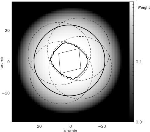
Figure 4: Weight map of a DIRBE healpixel. This represents the probability for a star to contribute to the healpixel flux as a function of its position in the sky. The diamond shape represents the particular healpixel (here in the Taurus–Perseus region). The thick pillow-like contour delimits the region inside which all stars contribute in all individual observations (probability = 1). The dashed circles represent the probability = 1 for a star to contribute for the given pointing. Each of the four circles is centered at one of the four corners of the diamond shape. The outer thick circle is the probability = 0.5 for a star to contribute.

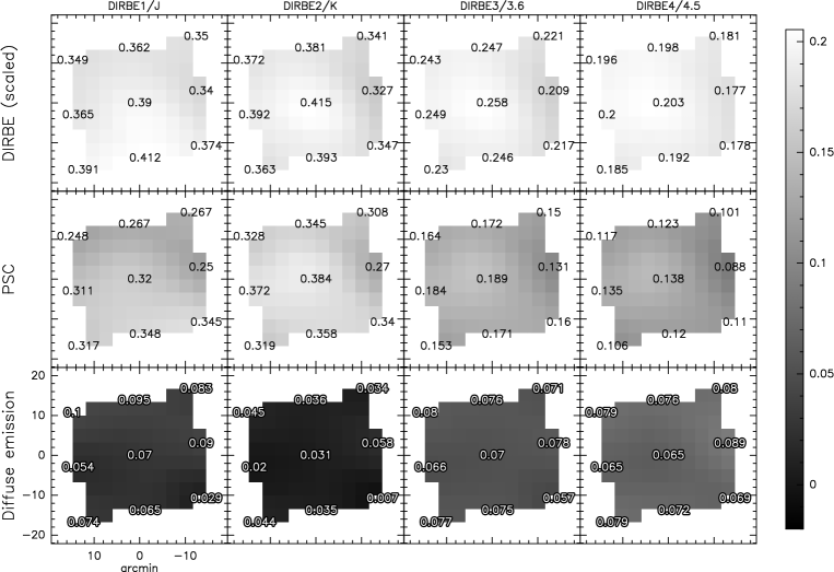
Figure 5: The nine nearest healpixels towards a single Taurus–Perseus position (here, L1544). Each column corresponds to a wavelength. Top row is the DIRBE values (rescaled respectively to 2MASS or Spitzer units), middle row the star flux contribution (PSC) and bottom row the remaining diffuse emission I${}_{\mathrm{diff}}(\lambda)$. Grey scale and values are given in MJy sr^-1

The second method is based on the flux subtraction of the sources by summing them from 2MASS and WISE point source catalogs (Skrutskie et al. 2006; Cutri et al. 2012a, b). This has been done in several studies that tried to estimate the CIRB and we basically apply the same method as described in Levenson et al. (2007). The DIRBE HEALPix maps are made of pixels of equal area but of different shape (healpixels, Górski et al. 2005). Each healpixel contains the average of all pointings that fall inside that pixel, for all orientations since DIRBE observed each position in the sky many times with different position angles. The probability that a star contributes to the measured flux of a healpixel is therefore not trivial to evaluate (Levenson et al. 2007). For each cloud direction, the healpixel shape is different and we have to compute the probability map of the stellar contributions for each of them separately. We start from the probability that a star falls inside the DIRBE pixel for any position angle (this probability is 1 inside a 20′ radius and 0 outside a 28′ radius) and we add together the DIRBE pixel probability map for all positions inside the healpixel shape (discretized to the arcmin level). The resultant weight map is renormalized to unity in its center. Such a map is displayed in Fig. 4 for the Taurus–Perseus region. This weight mask is applied to a catalog of point sources to compute their contribution to the healpixel.

For each cloud of interest, we retrieve the DIRBE pixel value that covers the cloud and its eight neighbors, and the shape of that particular healpixel. We compute the weight map as described above and retrieve the 2MASS and WISE point source catalogues of the corresponding region (from the Vizier database). The point source fluxes are obtained by using the zero flux reference of Jarrett et al. (2011) for WISE and of Cohen et al. (2003) for 2MASS. Then, for each band, individual stellar contribution is respectively converted to Spitzer fluxes or kept in 2MASS fluxes, summed with the appropriate weight maps and subtracted from the DIRBE pixel value (scaled to Spitzer or 2MASS fluxes). The number of point sources considered varies from 5,000 in the 2MASS catalogue at high galactic latitude (36°, L183) up to 30,000 sources in the WISE catalogue for lower latitudes ($-$14°, Chameleon). An example measurement using nine pixels along with a point source contribution estimate is shown in Fig. 5.

The results for the four regions discussed in this paper are summarized in Table LABEL:tab:Iback_table. For each line of sight and wavelength, we give the value of the central pixel, the nine pixels average value and the dispersion. The I_diff values obtained from individual lines of sight have been chosen to be representative of the complete region for the Taurus–Perseus complex, the southern part of Chameleon and L183 direction. The Cepheus region is more heterogeneous. It shows a gradient in the Galactic Plane direction and has to be considered more cautiously (Fig. 6).

One can note that the CIRB contribution (eq. 1) is negligible compared to I_diff in J but is in the 50-100% range in K. It represents $\sim$ 25-50% of the diffuse flux at 3.6 $\mu$m and 4.5 $\mu$m. At 5.8 and 8 $\mu$m, the star contribution is considered to be negligible and the background emission is directly measured from the interpolated DIRBE fluxes in these bands as explained in Sect. 3.2.1.

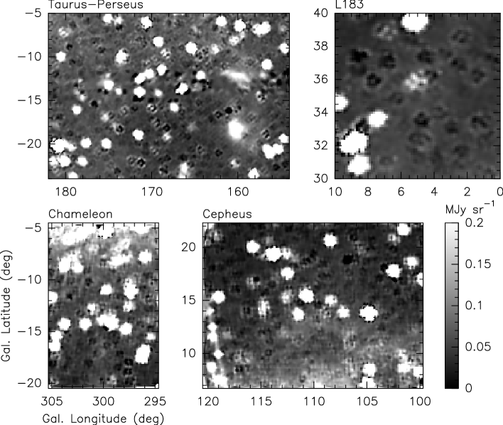
Figure 6: Maps of the diffuse emission I_diff at 3.6 $\mu$m for the four regions obtained with the second method at the DIRBE resolution.

The method is efficient but can become inaccurate when very bright stars enter the field since their flux is not always correctly estimated in the WISE or 2MASS catalogs though it represents a major fraction of the total flux in the DIRBE pixel. For a discussion about non-linearities and saturation due to bright stars in the determination of the photometry, the reader is referred to the explanatory supplements of the WISE and 2MASS missions. The adopted correction also assumes that the completeness of the input catalogs is similar to the depth to which point sources are removed in our analysis of the diffuse signal. Indeed, the faint end of the source distribution is only a few kJy sr^-1 in J and K and even less at coreshine wavelengths (Levenson et al. 2007). The uncertainty on the method can be estimated from the fluctuations between the nine adjacent pixels and from the fact that no pixel should show a flux lower than the CIRB flux (Table LABEL:tab:Iback_table). The zodiacal light subtraction we use is also challenged by some authors and the result slightly depends on the adopted zodiacal light correction (see Table 5 in Levenson et al. 2007).

The two methods are qualitatively in agreement at 3.5 and 4.9 $\mu$m but not in J and K bands. While the first method supposes that all the J band flux is due to the stars, the second method finds a sizable fraction of the flux to be due to the diffuse light (10 to 25 %). This is expected since the standard interstellar grains in the diffuse medium are more efficient at scattering light at 1.2 $\mu$m than at 2.2 $\mu$m. It is in the K band that the diffuse contribution reaches a minimum. The diffuse emission fraction is also higher in the 3.5 and 4.9 $\mu$m bands since the stellar contribution decreases with increasing wavelength. When we obtained results below the CIRB intensity we replaced I_diff by the CIRB intensity in our models. This happened only in the Cepheus direction, for the K, 3.6, and 4.5 $\mu$m bands. The second method is more reliable at getting the measurement of $\mathrm{I_{diff}(\lambda)}$ when we investigate a particular direction (modeling a cloud) while the first is more useful in exploring what happens at Galactic scales in the MIR.

The measurement of $\mathrm{I_{\mathrm{diff}}(\lambda)}$ is not the only parameter we need to know to reconstruct the absorption part of the final map; the proportion of the diffuse emission which is in front of our cloud (foreground = fg) and the one which is behind (background = bg) is a key element too (see eq. 1). These quantities are directly linked to the proportion of dust in the diffuse medium located in front and behind the cloud. Their evaluation is based on a model of dust in our Galaxy up to 300 pc by Lallement et al. (2014, bg1) and has to be taken as an indication rather than a precise value. That is why, for certain lines of sight, and when possible, we also used an other estimate based on a different method by Marshall et al. (2006) to evaluate the uncertainty on the fg and bg values. This method, known to be unreliable below one kpc, has been refined and give better approximations at smaller heliocentric distances (Marshall et al., in prep, bg2).

At the end, it is the product of $\mathrm{I_{\mathrm{diff}}(\lambda)}$ with the bg value that gives $\mathrm{I_{\mathrm{back}}}$ (eq. 1). The contrast level of the emergent flux (I_final) in final model maps will depend on this I_back value as follows:

$$\mathrm{I_{\mathrm{final}}=(I_{\mathrm{sca}}+I_{\mathrm{back}}*\mathrm{exp(-\tau)}\-)-I_{\mathrm{back}}\-.}$$ (3)

with I_sca the scattered light image, $\tau$ the integrated extinction opacity map, both obtained from the radiative transfer code, and $\mathrm{(I_{\mathrm{sca}}+I_{\mathrm{back}}*\mathrm{exp(-\tau)}\-)}$ the transmitted signal from the cloud. The focus on four different regions allows us to explore different ($\mathrm{I_{\mathrm{diff}}}$, bg) pair values and see the impact on the emergent intensity in the modeling.

3.3 Molecular cloud content

3.3.1 Cloud model

Because modeling in 3 dimensions is mandatory (Appendix A), we chose to use a general 3D shape that represents most of the data clouds. An inclined ellipsoid has been taken as the cloud model. This cloud model was built to correspond to 40 pixels for a cloud radius (core+envelope) equal to 16000 AU (Fig. 7). This corresponds to a resolution ranging from 2″ to 7″ depending on the distance of the region, a few times the Spitzer resolution. Because the coreshine varies slowly through the cloud (red area Fig. LABEL:fig:L183_sex) and because we are interested in the surface brightness (in MJy sr^-1), this resolution is not crucial. We made a compromise by limiting the total number of cells (with a size of 104$\times$104$\times$104 cells) to reduce the computational time. However, we keep enough cells to dedicate reasonable physical space to the cloud in our modeling cube while keeping some room for the external part. This also explains why we chose a jump at lower density to the envelope instead of a smooth variation. This has a minor impact on the modeling.

The minor axis has been designed to be half the major axis, and the inclination angle is 60° to see a possible gradient effect as a function of the direction of the Galactic Center. The adopted density profile for the core is a Plummer profile adapted to an ellipsoid (from Doty et al. 2005 and Whitworth & Ward-Thompson 2001)

$$n(x,y,z)=\frac{n_{0}}{1+\left[\frac{r}{a_{0}}\right]^{\alpha}},$$ (4)

with:

$$r=\sqrt{\frac{x^{2}}{a^{2}}+\frac{y^{2}}{b^{2}}+\frac{z^{2}}{c^{2}}}$$ (5)

where $n$ is the number density, $n_{0}$ is the reference density, $a_{0}$ the radius associated with $\frac{n_{0}}{2}$, $(x,y,z)$ defines the position, $(a,b,c)$ are parameters specifying the shape of the ellipsoid, with an index of $\alpha$ = 2.5. Generally used on a sphere, this type of profile (Fig. 7) is common and realistic for simple molecular clouds like L1544 in the Taurus–Perseus region (Doty et al. 2005).

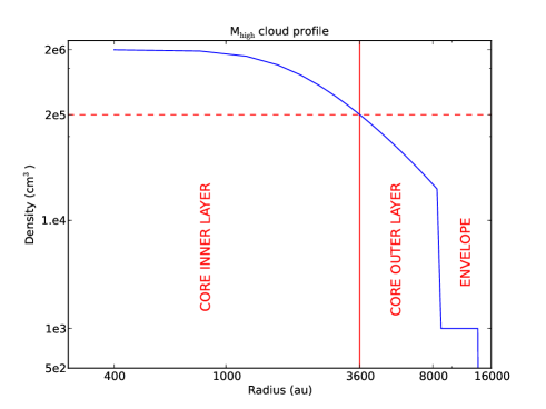
Figure 7: Cloud profile for the second cloud model (M_high) with a central density of 2 $\times$ 10⁶ cm^-3.

While the detailed shape does not really matter for our toy cloud model, the column density has to be more representative of the range of our observations. We defined two models, one with a central density of n₀(H₂)= 2 $\times$ 10⁶ cm^-3 (M_high = 1.5 M_☉) and another one with n₀(H₂) = 5 $\times$ 10⁵ cm^-3 (M_low = 0.4 M_☉) which gives a peak column density of 9.2 $\times$ 10²² cm^-2and 2.3 $\times$ 10²² cm^-2 respectively, and we assume a gas-to-dust ratio of 133 (Compiègne et al. 2011). The 3D cube model of more than one million cells is divided in two regions : an envelope and a core. The envelope, of constant density (1000 cm^-3), is always filled with a standard diffuse grain size distribution since NIR studies seem to be able to reproduce scattering in the outer parts of the investigated clouds with such distributions (Juvela et al. 2012). The core itself is divided in two parts of approximately equal thickness (Fig. 7) in which different grain characteristics are tested. The threshold between the two core layers is situated at density 2 $\times$ 10⁵ cm^-3 (for M_high), and 5 $\times$ 10⁴ cm^-3 (for M_low). Grain property gradients can thus be investigated from the envelope standard distribution to the inner core evolved grains.

3.3.2 Dust properties

Table 3: The different types of modeled grains and their properties.

Grain model name	amin	amax	acut	$\langle$a$\rangle$
	nm	$\mu$m	$\mu$m	nm
DustEm extended
aSil / CBx2	4	2	0.2/0.150	15.37 / 25.2
Cx.2	4	2	0.2	28.25
aS25 / Cx25	4	2	0.25	16.12 / 30.9
aS.3 / Cx.3	4	2	0.3	16.76 / 33.24
aS.4 / Cx.4	4	2	0.4	17.8 / 37.3
aS.5 / Cx.5	4	2	0.5	18.65 / 40.8
aS.6 / Cx.6	4	2	0.6	19.37 / 43.87
aS.7 / Cx.7	4	2	0.7	19.99 / 46.59
aS.8 / Cx.8	4	2	0.8	20.55 / 48.9
aS.9 / Cx.9	4	2	0.9	21.06 / 50.75
aS1m / Cx1m	4	2	1.0	21.52 / 52.14
aS2m / Cx2m	4	5	2.0	24.72 / 70.56
aS5m / Cx5m	4	9	5.0	29.12 / 97.18
S10 / C10	10	2	0.15	31.44 / 43.47
S20 / C20	20	2	0.5	66.1 / 106.88
S50 / C50	50	2	1.0	154.72 / 236.4
Other bare grains
WD31 (Si/Gra)	0.35	0.3/1.0	0.25/0.4
WD55 (Si/Gra)	0.35	0.3/1.5	0.25/0.6
WD55B (Si/Gra)	0.35	0.3/6.0	0.25/3.
ORNI2	0.1	0.6	0.3
With ices
ORI2	0.1	0.6	0.3
ORI3	0.1	2.5	1.2
Porous	$\rho$	$\alpha$	acut
	g cm-3		$\mu$m
YSA 0%	2.87	-2.4	0.234
YSA 10%	2.59	-2.4	0.242
YSA 25%	2.16	-2.4	0.256
YSA 40%	1.72	-2.4	0.276
Fractal				a
				$\mu$m
MIN0.2				0.2
MIN0.8				0.8
MIN1.2				1.2
MIN2.4				2.4
MIN4.0				4.0

The main dust models used in this paper are based on an extrapolation of standard grains able to fit the observations in the diffuse medium (comprised of a mixture of silicates and carbonaceous grains, in the classical proportion of 3/4 to 1/4, respectively) from DustEm. DustEm is a software package implemented by Compiègne et al. (2011) which is able to compute the dust emission from a spherical grain size distribution and grain optical properties (obtained internally by using Mie theory and the IDL code DustProp). Since we focused our study on scattering and absorption and not emission, DustEm is used as a tool to average the grain properties on their size distribution wavelength by wavelength. In each cloud layer (see Sect. 3.3.1), we mixed the two dust species and adjusted their size distributions independently. This hypothesis is justified by the fact that the two species are supposed to be able to coagulate in separate ways (deduced from the extinction curves, Hirashita & Voshchinnikov 2014).

Our extrapolation starts from the biggest grain size distributions of DustEm (hereafter aSil and CBx2 according to Compiègne et al. 2011 notations, Table 3). The goal is to investigate to what extent grain growth inside molecular clouds, especially coagulation, is able to explain the coreshine observations. For both species, 1 $\mu$m grains are known to be sufficiently efficient in scattering and producing coreshine (Pagani et al. 2010 and Fig. 8) but some questions remain: is the suppression of the smallest grains required to observe coreshine? Is there a size limitation for the distribution? What is the influence of the change of the slope of the power–law or of the complete dust distribution itself? What is the impact of taking into account ice mantles and fluffy grains?

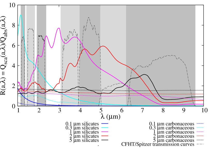
Figure 8: Ratio of the scattering and absorption efficiencies for individual grain types and grain sizes. The grain properties come from Compiègne et al. (2011). The grey bands delineate the different filter bandpasses (CFHT J, H, Ks, Spitzer 3.6, 4.5, 5.8, 8.0 $\mu$m).

In this perspective, we tried different short cutoffs (minimal size for the grain size distribution: a_min) and long exponential cutoffs ($e^{-(a/a_{\mathrm{cut}}-1)^{2}}$, where a is the grain radius, a_cut the cutoff radius) which applied on the original size–distribution power–law (Compiègne et al. 2011, Table 3). In particular, the index of the original power–law is $-$3.4 for the silicates and $-$2.8 for the carbonates. The a_min value evolves from 4 nm (aSil, CBx2) up to 50 nm (C50, S50) while also the high cut–off value changes. Nevertheless, we also chose to compare grain size distributions with the same high cut-offs and different short cut-offs to test the influence of small grains (e.g. from Cx1m to C50). All the grain size distributions between CBx2 and Cx1m, as well as aSil and aS1m, have also been used to reproduce a smooth increase in size through the cloud (GRAD model hereafter). The change of the whole distribution itself has been investigated thanks to the use of different grain types from the litterature (Weingartner & Draine 2001, Ormel et al. 2009) as well as the porosity (Ysard et al. 2012) and the fractal dimension (Min et al. in prep).

For all the grain models, the optical properties are averaged in each cell of the cloud. DustEm provides us with averaged parameters for each grain size distribution taking into account the grain distribution law and the dust mass for each species. Therefore, we have to consider three averaged parameters: the mean scattering efficiency $\langle$$\mathrm{Q_{sca}}$$\rangle$, the mean absorption efficiency $\langle$$\mathrm{Q_{abs}}$$\rangle$, and the mean phase asymmetry factor $\langle$$\mathrm{g}$$\rangle$. This phase function, the probability for a photon packet to be scattered in a given direction, is well–approximated by the Henyey–Greenstein expression

$${\mathrm{P_{\textrm{HG}}(\mu)=\frac{1}{2}\frac{1-\langle g\rangle^{2}}{(1-2\langle g\rangle\mu+\langle g\rangle^{2})^{3/2}}}},$$ (6)

with

$$\mathrm{\mu\ =cos(\theta),}$$

and

$$\mathrm{\int_{-1}^{1}\!P_{\mathrm{HG}}(\mu)\,\mathrm{d}\mu=1,}$$

which is accurate enough for spherical grains up to a form factor $x=2\pi$$\langle$a$\rangle$$/\lambda$ equal to 10, with $\langle$a$\rangle$ the mean size of the grain size distribution and $\lambda$ the wavelength. In this paper, the form factors of the size averaged dust models vary from 0.04 to 0.4 at 3.6 $\mu$m (Table 3). Only the axial backward scattering might not be taken sufficiently into account. The full radiative transfer equations are described in Steinacker et al. (in prep.). Nevertheless, the averaging process on the whole size distribution has been tested by comparing a full distribution and the same distribution cut in three parts and put together in the same cell. No difference could be found providing the size distribution discretization had been increased up to 600 steps in DustEm.

To understand the competition between scattering and absorption at NIR and MIR wavelengths, it is important to look at the individual properties for the different sizes and grain components (Fig. 8). One can notice from Fig. 8 that for a given total dust mass, $\langle$Q_sca$\rangle$ increases faster than $\langle$Q_abs$\rangle$ when $\langle$a$\rangle$ increases. This is undoubtedly linked to the emergence of coreshine in dark clouds (Steinacker et al. 2010). However, real clouds present a mixture of different grain types and grain sizes which imply some degeneracy. They are partly removed by modeling the cloud at several discrete wavelengths (from J band to 8 $\mu$m).

Because Compiègne et al. (2011) grains are not the only ones able to explain the observations in the diffuse medium, and in order to explore beyond spherical grains, we added a sample of dust grain varieties. In our grid of models, silicate and graphite mixtures (Weingartner & Draine 2001, WD31, WD55, WD55B), porous grains without ices (Ysard et al. 2012, YSA 0%, YSA 10%, YSA 20%, YSA 40%), monomer fractal aggregrates with different sizes (Min et al. in prep., MIN0.2, MIN0.8, MIN1.2, MIN2.4, MIN4.0) or compact agglomerates with ices (Ormel et al. 2009, ORI2, ORI3) and their counterpart without ices (Ormel et al. 2009, ORNI2) were included with different maximal sizes (see Table 3 and references for more details). We do not attempt to provide a review of all the grain types available in the literature, among which a-C:H grains (Jones 2013), and iron inclusions in silicates (Jaeger et al. in prep) are other possibilities. The goal is to open the scope of what kind of grains will be suitable to explain our observations.

4 Results

The coreshine strength is linked to the grain properties and to the environmental conditions. The modeling has to deal with the absolute coreshine intensity which is a contrast problem and a competition between scattering and absorption. These extinction processes are linked to the dust properties, and in particular to the grain size distribution. However, these properties are degenerate when considering a single wavelength. Therefore, we adopted a multi–wavelength approach in which the albedo variation between wavelengths, dependent on the dust population itself, is well–characterized by intensity ratio measurements.

In Sect. 4.1, we present the measurements of the two key quantities, the 3.6 $\mu$m intensity and the coreshine ratio (between 4.5 and 3.6 $\mu$m wavelengths) for the observational sample of the four regions. In Sect. 4.2, we expose the conditions to make coreshine appear and retrieve the correct absolute intensity from modeling while, in Sect. 4.3, we detail the use of the different intensity ratios as a tool.

4.1 Surface brightness and coreshine ratio in observations

We investigated two thirds of the detected coreshine cases, located in four different directions of the Galaxy, to look for regional variations, either spatial or physical. The two main regions we ignored (Orion/Monoceros and $\rho$ Oph) present an equal number of detections and non-detections, which indicates that these regions might be more sensitive to specific local conditions and are beyond the scope of this work. Figure LABEL:fig:Observations gives the 4.5 $\mu$m / 3.6 $\mu$m ratio as a function of the 3.6 $\mu$m intensity for all the sources (values are given in Table 1). The horizontal bars represent a $\pm$ 10 % uncertainty that is a conservative value of the error budget, which is dominated by the background removal, while the vertical bars represent the range of ratios around the peak ratio value (Sect. 2.3 and Fig. LABEL:fig:L183_sex). Some of the weakest sources (21) have a signal–to–noise ratio at 4.5 $\mu$m which is too low to safely estimate the coreshine ratio. Their 3.6 $\mu$m intensity ranges from 10 to 40 kJy sr^-1. For the others, the 3.6 $\mu$m intensity ranges from 21 to 390 kJy sr^-1, and their ratio from 30 to 110 %. Starless cores are in a narrower range, 10 to 100 kJy sr^-1 and ratios from 35 to 51 % (the L1517C case – 53 % – is weak and noisy and probably not different from its neighbors, L1517 A and B – 51 %). This upper limit of $\sim$ 50 % is well–explained by the fact that the incoming DIRBE illumination ratio is only 70 % at 4.5 $\mu$m with respect to 3.6 $\mu$m and that the scattering efficiency of grains up to 1 $\mu$m  is always lower at 4.5 $\mu$m than at 3.6 $\mu$m (Fig. 8). On the contrary, the stronger and redder coreshine flux of many sources with local or embedded Young Stellar Objects (YSOs) is clearly linked to the YSOs themselves which provide more photons than the ISRF locally, with a much redder color due to their dust cocoon.

However, some of the sources with nearby or embedded protostars may remain comparable to the starless cores. There are three possible reasons: the source is i) too weak (like the VeLLO – Very Low Luminosity Object – in L1521F), ii) too deeply buried (like the strong jet driver L1157–mm/IRAS 20386+6751), or iii) too far outside the cloud though this is difficult to estimate since the relative position of the cloud and the YSO are not known with enough precision along the line of sight (see Table 1 and references therein). This is the case for the L1157 region which shows a low ratio (41 %) near the embedded driving source of its strong outflow, and partly along the southern outflow itself, while it displays a high ratio (71 %) just beyond the tip of this southern outflow where no YSO can be seen. A possible explanation is that the outflow provokes a shock region (B1 seen in H₂) which emits in the MIR with a 4.5 to 3.6 $\mu$m ratio of 2.5 that might change the coreshine ratio of that part of the cloud.

For several sources the embedded object has a limited range of influence and if the core is extended, a multimodal ratio distribution appears (Fig. LABEL:fig:ecc815). In the cloud (G303.72-14.86) presented in Fig. LABEL:fig:ecc815, the strongest source is at the top end of the cloud, inside the blue polygon, and two other interacting but weaker stars are situated just below, inside the red polygon. Sources themselves are masked, hence the white spots. The situation for YSOs is quite complex, because other physical effects (e.g dust alignment due to polarization - Chapman et al. 2013 - and/or dust destruction) could have a profound impact on the coreshine effect. Indeed, for L1152 and L1228 there is the suggestion from NIR (JHKs) and MIR (Spitzer) that there are regions where shocks have destroyed grains (Chapman et al. 2009), thus potentially affecting the coreshine effect. This is probed by the fact that even though the radiation is enhanced by the local source, the 5.8 $\mu$m band remains in absorption which would not be possible with too large grains.

Though the scattering effect does not seem to change much across the Galaxy as shown in Pagani et al. (2010, their Fig. 4), we expected to find some difference between the four regions when taking into account the background and the contrast problem (see next Section). Of course, Pagani et al. (2010) indicate scattering effects towards the Galactic center while we will see hereunder it is impossible to see any but Fig. LABEL:fig:Observations clearly shows that away from the Galactic plane and bulge, there is no difference between the regions either in absolute flux or in ratio values while the background values I_back vary by a factor up to around four between Cepheus and Taurus–Perseus (Table LABEL:tab:Iback_table). Moreover, the main incoming radiation field, from the Galactic center, is either behind the cloud, on its side or behind the observer (in the Taurus–Perseus direction, which implies some efficient backward scattering for anti-center cores, Steinacker et al. 2014a). The dispersion seems to be dominated by individual cloud properties instead, with little sensitivity on the coreshine ratio.

Finally, the very high proportion of coreshine cases in these regions is an interesting question. Either the grown grains are already present in the local diffuse medium of these regions and become apparent when the dust is concentrated enough or the grains coagulate relatively fast once the clouds are formed and before the turbulence dissipates in the cores (Steinacker et al. 2014b). In the first case, the presence of the grown grains in the diffuse medium might explain the excess of emission at 3.6 and 4.5 $\mu$m seen by Flagey et al. (2006). This could be checked by examining the differential MIR spectrum on lines of sight sampling the diffuse medium inside and outside the Gum/Vela region for which the low number of cores with coreshine and the high presence of PAHs may indicate the erosion of large grains by the blast wave (Pagani et al. 2012). The second hypothesis would require the modeling of grain growth together with cloud contraction and turbulence dissipation.

4.2 Coreshine emergence

To study the coreshine emergence as a function of the galactic position, we use the all-sky background map obtained after stellar subtraction (following first method, see Sect. 3.2.2) and we have done the modeling for several elevations towards the Galactic center direction, 90° from it (in longitude) and towards the Galactic anticenter direction (Fig. LABEL:fig:GC) for a given cloud (M_low) and grain size distribution (aS1m/Cx1m) models. We easily explain that it is not possible to observe coreshine in the galactic plane because of the strong background field, even with favorable grain properties (grain size distribution up to 1 $\mu$m grains and $\langle$Q_sca$\rangle$ greater than $\langle$Q_abs$\rangle$). For a galactic longitude ($\mathrm{l}$) of 0°, the bulge dominates the background field so strongly that coreshine is not able to appear until a galactic latitude ($\mathrm{b}$) around 10°. On the contrary, in the anti-center direction coreshine is able to appear rapidly with elevation, as low as $\mathrm{b}$ $\geq$ 3°. When the main illumination field comes from behind, at small angles, coreshine appears for higher background values than for other illumination directions ($\sim$300 kJy sr^-1instead of $\sim$120 kJy sr^-1, Fig. LABEL:fig:GC). The values are compatible to what was found by Steinacker et al. (2014a), here we also confront these criteria directly to the detections. This modeling correctly explains the observations (Fig. LABEL:fig:planck) but the $\mathrm{b}$ values given in Fig. LABEL:fig:GC have to be taken qualitatively since the values can change with the presence of local sources, the grain properties and the background proportion estimates. Finally, of all the clouds that contain enough micron-size grains to efficiently scatter the MIR light, only those outside the Galactic plane are detectable via their coreshine emission and the 50$\%$ detection of positive coreshine cases (Pagani et al. 2010, Paladini et al. in prep.) is only a lower limit in terms of grown grains in clouds.

Beyond the galactic plane contrast problem, clouds will also appear in absorption if $\langle$Q_sca$\rangle$ is lower than $\langle$Q_abs$\rangle$. Nevertheless, there are not a lot of cases in real absorption outside of the Galactic plane in our data collection (Table LABEL:tab:sources). Scattering is always present in dark clouds, even when the cloud is seen in absorption. The coreshine phenomenon starts to appear when the scattering signal is able to exactly compensate the extinction of the background field. Incidentally, clouds would totally disappear if this equilibrium was reached at MIR wavelengths. The coreshine phenomenon could be understood either by the presence of large grains ($\sim$ 0.5 – 1 $\mu$m) or a stronger local radiation field which would enhance only I_sca (eq. 3). The enhancement of the local radiation field has to be considered cautiously since it has to be consistent with far–IR emission of the clouds. Here, we are not refering to embedded YSOs but to the large scale local radiation field surrounding starless cores. Incidentally, Evans et al. (2001) show that for a selection of prestellar cores in Taurus and $\rho$ Oph regions, far-IR observations seem to require a lower ISRF than standard to be fitted. On the contrary for the $\rho$ Oph region, Roy et al. (2014) argue that the ISRF is one order of magnitude higher than standard.

At 5.8 and 8 $\mu$m, all the clouds of the cold Spitzer survey (Pagani et al. 2010) appear in absorption. While at 8 $\mu$m, this is partly due to the 9.7 $\mu$m silicate absorption feature wing that intercepts half of the 8 $\mu$m filter width, at 5.8 $\mu$m, it is only due to the background field strength. Indeed, the diffuse part I_diff increases globally more and more with the wavelength (Table LABEL:tab:Iback_table) in the IRAC bands range as can be seen in Flagey et al. (2006). In parallel to this increase of the diffuse background field, the scattering efficiencies drop. This provides additional constraints, in particular our modeling can eliminate the grain models for which the 5.8 $\mu$m map shows emission. This is especially true for distributions which include grains in the range 2–5 $\mu$m for both silicates and carbonaceous grains (aS5m/Cx5m) and puts an upper limit for the grain size based on the 5.8 $\mu$m diagnostic deep inside the core. Nevertheless, this limit in size has to be taken cautiously since it is dependent on the grain size distribution law and on the grain composition. It has to be understood as un upper limit on the abundance of grains larger than 2$\mu$m, and for example, the WD55B distribution stays compatible with absorption at 5.8 $\mu$m. The 8 $\mu$m map always appears in absorption in our simulations and is not, as expected, sensitive to the grain properties but could be used to constrain the silicate column density.

4.3 Intensity ratios as discriminants

We aim to separate the grain models according to their ability to explain the observed intensity ratios between bands. We start from the coreshine ratio (4.5/3.6) and extend the method to a comparison between NIR and MIR bands (K/3.6) and to NIR ratio (J/K ratio). The four modeled directions cover a range of local properties like the Galactic Center direction, and the differential local background field $\mathrm{R}_{\lambda 1/\lambda 2}(\mathrm{I}_{back})$ = I_back($\lambda_{1}$) / I_back($\lambda_{2}$) (Table LABEL:tab:Iback_table).

To measure the ratios, we took the median value inside a polygon on the simulated map ratios. We obtain the model uncertainty by comparing these ratios computed with different I_back estimates (obtained with the second method, Sect 3.2.2), namely the center pixel values versus the nine pixel average values, and the two bg estimates (bg1, bg2) (Table LABEL:tab:Iback_table). The suitable grain models are the ones which satisfy all the criteria taking into account the uncertainties on the background variation. For the M_low cloud model (see Section 3.3.1), the chosen polygon is very central and corresponds to a mean value of A_V = 23 mag (assuming Rv = 5.5) while the mean polygon extinction for the M_high model is about A_V = 21 mag chosen to be between the two layers and outside the internal depression.

4.3.1 Grain properties deduced from the coreshine ratio

We plot the coreshine ratio derived from the model calculations as a function of the 3.6 $\mu$m coreshine intensity for all the grain models and separately for the four modelled directions corresponding to the observed regions (Fig. 12 to 15). All the models that do not show coreshine at both 3.6 and 4.5 $\mu$m are not displayed on the ratio plots, especially WD31, ORI2, ORNI2, YSA models. Figure 12 confirms that the two different cloud models that investigate different zones with close averaged visual extinction give coherent results and that we correctly represent the observational range. Moreover, the plots are not really sensitive to the background proportion itself concerning the coreshine ratio range (bg = 95 or 75 % for the Taurus–Perseus region, Fig. 12, and bg = 75 or 50 % for the L183 direction, Fig. 13). However, this implies some degeneracy in the grain property solutions for some regions (Fig. 12). Conversely, regions where the I_sca term is dominant (eq. 3, 13) give more reliable results. This regime is reached for the L183 and Cepheus regions. For the following, we keep the estimates by Lallement et al. (2014) as a reference (bg1, Table LABEL:tab:Iback_table).

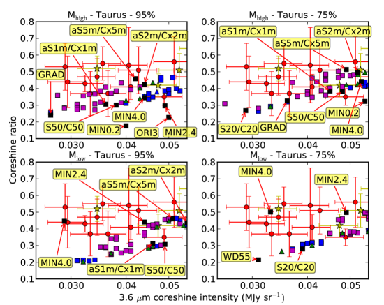
Figure 12: Coreshine ratio versus 3.6 $\mu$m intensity in the Taurus–Perseus direction. Zoom on the starless core cases, full range is displayed in Fig. 14 - Difference between M_high (upper row) and M_low (lower row) modeling without internal source for the two background fractions (95%, bg1, left, 75%, bg2, right). OBSERVATIONS - red circles: starless cores; yellow stars: cores with YSOs. MODELS - black squares: single grain population; blue squares: carbonates bigger than silicates in at least one of the two layers; purple squares: silicates bigger than carbonates in at least one of the two layers; green triangles: everything else. Grain model names refer to Table 3 for spatially constant grain size distribution.

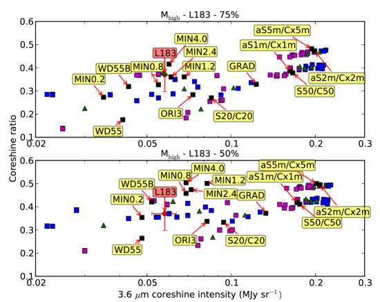
Figure 13: Same as Fig. 12 in L183 direction with the two background proportion estimates: 75% (bg1, top), and 50% (bg2, bottom).

The first question is to determine whether small grains have any impact on the coreshine modeling. We found that no differences appear between models which contain small grains between 4 and 10 nm and the ones without grains below 10 nm (from aSil to S10 grains and from CBx2 to C10, Table 3, LABEL:tab:solutions). Removing the small grains at constant dust mass has been tested up to 50 nm (S50, C50) and the results are very close to the ones with the same high cut–off (a_cut = 1 $\mu$m) but with a starting size of 4 nm (aS1m, Cx1m), especially when taking into account the uncertainties (see e. g. Fig. 13). The suppression of the smaller grains is therefore not mandatory in explaining the coreshine phenomenon because they do not contribute nor attenuate the signal significantly.

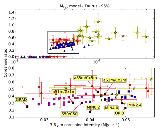
Figure 14: Top: observations, same as Fig. 12 in Taurus–Perseus direction. Blue triangles: all (undifferentiated) starless models. Bottom: zoom of the rectangle in the top image, symbols identical as in Fig. 12

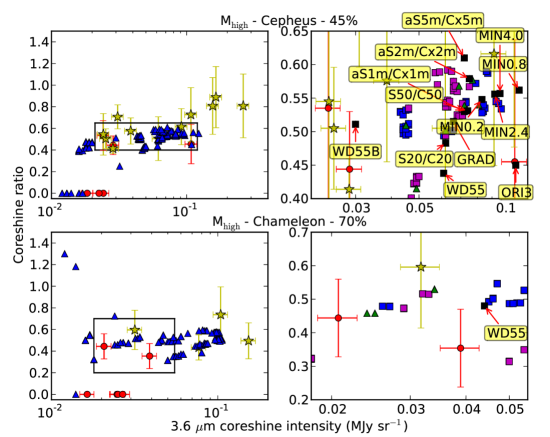
Figure 15: Same as Fig. 12 in the Chameleon and Cepheus directions: top Cepheus region, top right: zoom on the starless observational zone, bottom : Cepheus region with its zoom (bottom right).

On the other hand, we tested the large grain size increase beyond the expected limits (Andersen et al. 2013). The more the mean size of the distribution $\langle$a$\rangle$ increases, the more the 3.6 $\mu$m flux increases as well. The grain models on the right side of the ratio plots (Fig. 12 to 15) are those with the highest number of big grains, with an exponential cut-off at respectively 1 $\mu$m (aS1m, Cx1m), 2 $\mu$m (aS2m, Cx2m), or 5 $\mu$m (aS5m, Cx5m). However, when the high cut–off of the grain size distribution increases, the coreshine ratio starts to saturate and consequently grain growth alone is not a pertinent answer to increase the ratio beyond 50 % for the Taurus–Perseus and L183 regions (Fig. 13 and 14) and 65 % for Cepheus and Chameleon regions (Fig. 15). This is well–explained by the combination of three effects. Firstly, the integrated illumination field intensity at 4.5 $\mu$m deduced from the scaled DIRBE map is only 70 % of the 3.6 $\mu$m intensity. Secondly, an I_back lower at 4.5 $\mu$m than at 3.6 $\mu$m  helps to increase the ratio as explained in Sect. 4.2. Since the ratio values of I_back at 4.5 and 3.6 $\mu$m  $\mathrm{R}_{4.5/3.6}(\mathrm{I}_{\mathrm{back}})$, stay around 1 for the Taurus–Perseus region and L183 direction, they have a minor impact on the coreshine ratio, while the lower I_back(4.5 $\mu$m) towards Chameleon and Cepheus provides an explanation of why ratios near 65 % are reached (Fig. 15). In the third place, the ratio of the scattering and absorption efficiencies (Fig. 8) becomes flatter with wavelength for both grain types when the grain size is increased up to 5 $\mu$m.

We also confirm what has been found previously (Pagani et al. 2010, Steinacker et al. 2010). Classical diffuse medium grains (WD31 Weingartner & Draine 2001, aSil and CBx2) are not efficient enough to scatter in the MIR range. Indeed, it is well known that the ratio of visual extinction to reddening, R_V = 3.1, is not valid in dense, cold environment and R_V = 5.5 has been advocated (Weingartner & Draine 2001). This change of slope has been explained by grain growth. While the WD55 model gives a 3.6 $\mu$m coreshine flux between 20 and 50 kJy sr^-1 and a coreshine ratio about 20 %, depending on the local conditions (direction and I_back values), the WD55B model, which includes grains up to 10 $\mu$m in size, has been found promising by other observations in the MIR (Ascenso et al. 2012), and allows the coreshine ratio to increase up to 40%.

The previous results were obtained for compact spherical grains, and we also wanted to investigate the consequences of the fluffiness and of the coagulation, which has to be understood here as an agglomeration of smaller grains. We tested the evolved grains of Ormel et al. (2009), with or without ices, with different evolution time scales. We aimed to compare three different populations: i) a reference population, without ices, and an evolution time scale of 1 $\times$ 10⁵ years (ORNI2) which happened to produce no coreshine in the modeling, ii) another one starting from the same distribution and which evolved in the presence of ice mantles (ORI2), and iii) one which has grown during a longer timescale of 3 $\times$ 10⁵ years with ices (ORI3). Despite the presence of ices which favor coagulation, the ORI2 grain size distribution has not had enough time to reach a sufficient size (Fig. 1 in Ormel et al. 2009) to make coreshine appear as our models confirm. On the contrary, the ORI3 model traces some evolution like the WD55B model and shows a ratio compatible with the observations. For these two models, even though the ratio is compatible with the observations, the 3.6 $\mu$m flux is higher than observed which is acceptable since we could always adjust the cloud model in order to obtain the right flux with an identical ratio.

What appears from these comparisons is the fact that the first key role of ices is to favor growth but the 3.05 $\mu$m H₂O ice feature included in the edge of the IRAC filter could also play a role in increasing the coreshine ratio by changing the dust optical properties in the same way as the silicate feature enhances the absorption in the 8 $\mu$m filter. Since, without ices, the maximal size reachable in Ormel bare grain models is about 1 $\mu$m, comparable to the size obtained with the ORI2 model which produces no coreshine, it is not possible to compare the ORI3 model to the same size distribution without ices to disentangle the ice effect from the pure growth effect.

Scattering optical properties are supposed to be more sensitive to grain surface variations than absorption efficiencies. Consequently, we expect to see a direct impact of the flufiness on the coreshine. To calculate optical properties for fluffy grains, one can focus on the porosity with a simple approach where the proportion of silicates, carbonaceous grains, and vacuum in the grains do not depend on their sizes (Ysard et al. 2012) or one can explore the fractal dimension which means to focus on the dissymetry of the grains themselves build by agglomeration of monomers (Min et al. 2006). First, we studied the influence of the degree of porosity. The grains from Ysard et al. (2012) which could explain the far-IR emission in L1506C (Ysard et al. 2013), a condensation in a Taurus filament, are not efficient enough to produce coreshine at 4.5 $\mu$m while the 3.6 $\mu$m coreshine flux, about 13 kJy sr^-1 (compared to 33 kJy sr^-1, Table 1), does not vary from 0 % porosity to 40 % porosity (YSA models). Because porosity does not seem to be an answer to change the 3.6 $\mu$m coreshine intensity, and correspondingly the coreshine ratio, we tried to test the influence of fractal structure. As preliminary results, we tested fractal aggregates which show optical properties quite different from the compact spherical grains (Min et al. 2006). These fluffy monomer aggregates behave like small spherical silicate particles for the 9.7  $\mu$m silicate feature (Min et al., in prep.). Their sizes vary from 0.2 $\mu$m to 4 $\mu$m.

We had to approximate the real phase function provided by Min et al. by an equivalent asymmetry coefficient ($\langle$g$\rangle$, eq. 6). As it will be discussed below, the phase function is not expected to modify the coreshine ratio by much, especially because this approximation applies to both wavelengths. Indeed, the two coreshine wavelengths are close enough so that the respective variation in the phase function is weak. These grains are really promising since they do not necessarily imply a significant grain growth to produce a ratio about 40 to 50 % and could be an interesting answer for clouds which would not show much evolution from other tracers like depletion (e.g. L1521E Tafalla & Santiago 2004, Pagani et al. 2010). Furthermore, we find the same saturation of the ratio for the agglomerates as for pure spherical grains with grain growth, which seems to confirm a maximal size efficiency as can also be deduced from Fig. 8. Fractal aggregates behave like big spherical grains to produce a high coreshine ratio.

To limit the number of models, we restrained ourselves to two layers for the part dedicated to the core (Sect. 3.3.1), that is why we do not aim to fit exactly the observations. We introduced a finer slicing in 10 layers inside the core, filled with grains presenting a high cut-off increasing from 0.2 $\mu$m to 1 $\mu$m (GRAD model). We obtained a ratio close to a two-layer core model with a_cut of 1 $\mu$m (aS1m and Cx1m mixed) but with less flux (see e.g. Fig. 14), which is expected for the observations. This emphasizes again the fact that the cloud model and the way we fill it with several layers would act only on the absolute coreshine fluxes without modifying the ratio.

The phase function can slightly change the ratio especially if backward scattering becomes a non–negligible quantity. This is the case for the Taurus–Perseus region for which the main anisotropic radiation source (the Galactic Center) comes from behind us. Nevertheless, even if we consider an extreme case with $\langle$g$\rangle$ = -0.99 which corresponds to a probability of 75% to have axial backward scattering, the ratio in the Taurus–Perseus region, with the same $\langle$ Q_sca $\rangle$ and $\langle$ Q_abs $\rangle$ absolute values, increases from 35 to 40 % for grains up to 1 $\mu$m (aS1m, Cx1m). The variation is even smaller for less extreme probability changes. In the most extreme case, even if the ratio is not really sensitive to the phase function modification, the absolute intensity at 3.6 $\mu$m has been enhanced by almost a factor 30 to reach a few hundred kJy sr^-1. Incidentally, the emergence of coreshine for some dust models will be dependent on this parameter. We estimate that the Henyey-Greenstein approximation is satisfactory for most of the directions since the ratio is only slightly sensitive to phase function variations. We will investigate the impact on the absolute flux by considering the true phase function when we perform a full cloud model, especially for regions in the regime where the influence of I_back is dominant (Sect. 4.2).

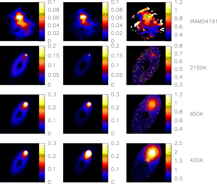
Figure 16: From left to right: IRAC 1 (3.6 $\mu$m), IRAC2 (4.5 $\mu$m), coreshine ratio. First row: analysis of IRAM04191 Spitzer observations. Next rows: Modeling in the dense case (M_high) for the three internal sources. Color scales are given in MJy sr^-1.

4.3.2 Impact of a local source

Since the presence of an embedded object is often found to enhance the coreshine ratio and the coreshine intensity in its vicinity (Table 1, Fig. LABEL:fig:Observations and LABEL:fig:ecc815), we explored the influence of a Class 0 or a Class I object in our model. The full treatment of a protostar reddened by its compact and dense dust cocoon is beyond the scope of this work. To investigate its possible effects qualitatively, we inserted blackbodies (stars) in the model with temperatures and fluxes typical of Class 0 or I objects at coreshine wavelengths. We ran the test with three different temperatures, 400, 950 and 2150 K and adjusted the flux accordingly. At 400 K, the 4.5/3.6 ratio is 3.8 and is representative of a Class 0 case as it could be observed for IRAM04191 (Chen et al. 2012). At 950 K, it is almost flat (1.2) and we obtain a flux and a coreshine ratio comparable to what could be deduced for a Class 0/I object like IRAS 04016+2610 or IRAS 04361+2547 (Robitaille et al. 2007). At 2150 K, it is typical of a solar type Class I protostar and its 4.5/3.6 ratio is 0.8, like IRAS 04325+2402 (Robitaille et al. 2007), close to the DIRBE all-sky ratio of 0.7. The Class distinction is not very important here since it depends very much on the geometry of the source and other factors that are beyond the scope of this paper. Several papers discuss these classification problems (e.g., Robitaille et al. 2007; Enoch et al. 2009; Kirk et al. 2009).

For the densest cloud model (M_high), we introduced, at the edge of the cloud, these three different stars. The test with the Class I object (2150K) shows a small enhancement of the coreshine ratio in the vicinity of the object (Fig. 16). With the Class 0/I object at 950K, the ratio is increased to $\sim$0.8. Finally, with the Class 0 object (400K), depending on its actual flux, the ratio can vary from below 0.5 for a negligible contribution (as in L1157 near the embedded object) to $\geq$ 2 if the local source flux dominates. We therefore can clearly reproduce the trend of the observations. However, we are not trying to make exact fits, and to go further in the modeling one has to constrain the local radiation field emanating from the embedded source to avoid the degeneracy between the grain properties and the local source flux and color.

Indeed, the question of whether the presence of an embedded protostar can be helpful or not in modeling the coreshine effect arises. If the protostar is weak and deeply embedded, its properties will be difficult to assess and its impact on the cloud scattered light will only add another degree of freedom. Similarly, if the source is clearly outside of the core, its distance to the cloud along the line of sight will remain a free parameter. If the YSO is clearly embedded in the cloud, but not too deeply, or in contact with it, so that its contribution can be measured directly, little uncertainty is added. This has three more advantages: Firstly, the ISRF becomes dominated by the local source and is therefore better constrained, secondly, as the scattered flux will be higher, the error due to the background uncertainty in the modeling becomes smaller and, thirdly the 5.8 $\mu$m criterium becomes even more constraining in enhanced ISRF conditions. Indeed, a stronger ISRF increases the capability to produce coreshine (either smaller grains can shine or big grains shine more). In a local stronger field, the non-detection of emission at 5.8 $\mu$m puts therefore a more stringent constraint on the abundance of grains above 1 $\mu$m as presented in Sect. 4.2. However, the presence of a Class 0 or Class I object indicates a more evolved cloud and, presumably, more evolved grains. Therefore studying starless clouds or protostellar clouds are both important and have both caveats.

4.3.3 Extension to the NIR

The information obtained from the coreshine ratio, which is more sensitive to the grain models than to the other free parameters, can be extended to NIR wavelengths. Specific studies on NIR scattering have been done before (Malinen et al. 2014 and references therein). Our approach assumes that the different wavelengths are close enough to investigate the same volume of the cloud and far enough to see a variation in the slope for the different grain types (Fig. 8). Because our NIR observations are limited to a few cases, we only set a range for the expected ratio values which we admit does not provide much constraint. Nevertheless we attempted to see if the multi-wavelength approach could lead to a sample of suitable grain models.

First, we studied the K  / 3.6 $\mu$m (= NIR/MIR) ratio as a function of the coreshine ratio towards L183 and the Taurus–Perseus complex. The observational range obtained for this ratio is between 3.5 and 6 for L183 and 3.2 and 7 for Taurus–Perseus region (Fig. 17 and 18). This eliminates models with a valid coreshine ratio but a NIR/MIR ratio which is too low (ellipse, Fig. 17). In both directions, the selected models correspond to relatively large grain size distributions, which is what we expected since the K band is supposed to sample a region close to the core (see Fig. 19 and Andersen et al. 2013). Nevertheless, when the grain size distributions contain too many large grains (aS2m/Cx2m, aS5m/Cx5m) the NIR/MIR ratio becomes too low. Actually, grain growth on spherical grains lowers the NIR/MIR ratio because when $\langle$a$\rangle$ increases, the K intensity increases but more slowly than the 3.6 $\mu$m coreshine intensity. This applies mainly to clumps with A_V $>$ 10 mag, when the K band already suffers significant saturation. In the same way, the fractal aggregates, even the 0.2 $\mu$m monomer aggregates, also seem to predict a NIR/MIR ratio that is too low. On the contrary, ice mantles (ORI3) give a higher NIR/MIR ratio and are one of the more suitable grains for the Taurus–Perseus region. In both directions, grain size distributions which contain bigger silicates than carbonates are more likely to be the ones able to explain the observations (purple squares - Fig. 17 and 18). Some spatially constant grain size distributions are also able to explain them, especially the ones up to 1 $\mu$m with or without ices (aS1m/Cx1m, ORI3). Finally, the L183 direction is well explained by silicates up to 1 $\mu$m and with different grain size distributions for the carbonates (from a high cut-off of 0.15 $\mu$m, CBx2, to 1 $\mu$m, C50) while the Taurus–Perseus direction can tolerate a larger variety of grains as a solution, for example model A is one with standard grains in the external core layer and grains up to 1 $\mu$m (S50/C50) in the inner layer (Table LABEL:tab:solutions). In this case only the second layer is visible in coreshine (Fig. 19) and almost the same region is emitting in K band while the J signal is more extended.

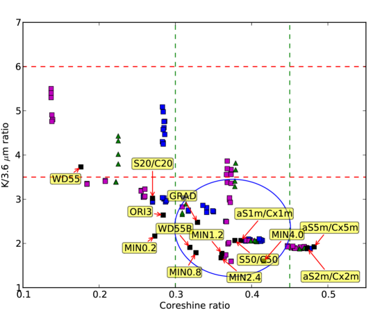
Figure 17: NIR/MIR ratio versus coreshine ratio plot for L183 for the M_high model. OBSERVATIONS: red dashed lines: observational range of the NIR/MIR ratio, green dashed lines: observational range of the coreshine ratio. MODELS: same as Fig. 13. Blue ellipse delineates the coreshine compatible grains which are eliminated from the NIR/MIR ratio.

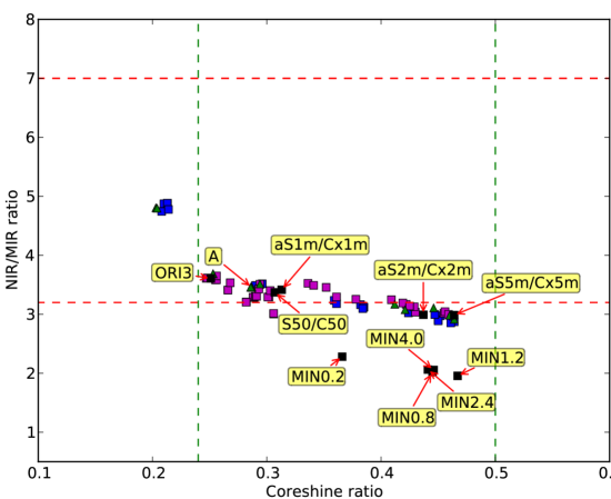
Figure 18: Same as Fig. 17 for the Taurus–Perseus region with the M_low model.

The simple cloud model we are using could be a limitation to investigating shorter wavelengths which are supposed to be more sensitive to the smaller grain part of the distribution contained in the extended envelope. Nevertheless we obtained interesting results about the J/K ratio (NIR ratio). The typical observational range obtained for the J/K ratio is from 0.3 to 3 and this ratio is highly position dependent which is well–reproduced in the modeling (model A, Fig. 19). Globally, it shows a bimodal distribution: one around 3 for the part dominated by the J region of emission and one below 1 for the central part dominant at the K wavelength. In particular, the model output median values for this ratio, which averaged this bimodal behavior, varies from 0.3 to 0.9 only (Table LABEL:tab:solutions), for the remaining suitable grains. Therefore it could not be used as an indicator to differentiate the models and is supposed to be more sensitive to the cloud structure than to the grain properties.

In conclusion, the preliminary constraints put by the multi-wavelength approach give us suitable grain models as solution for the Taurus–Perseus and L183 regions in standard ISRF illumination conditions. L183 ratios are well reproduced by grain models which contain bigger silicates or a mix between bigger carbonates in one layer and bigger silicates in the other layer while the Taurus–Perseus region admit also spatially constant grain size distribution models as solutions (Table LABEL:tab:solutions). In particular, grains which could explain the observations in the Taurus–Perseus region are globally bigger than the ones able to explain L183 observations. The addition of water ices lower the coreshine ratio but increases the NIR/MIR ratio and could be an answer for some cores in Taurus–Perseus region but has to be considered carefully. Bigger silicates have also tendency to increase the NIR/MIR ratio while decreasing the coreshine ratio, and carbonates increase the later and yield higher flux at 3.6 $\mu$m. In any case, grain composition have an important role to play and the classical spherical silicates/carbonates approach has to be modulated, for example the fractal dimension is a major actor even if it is not able to explain the NIR/MIR ratio alone for both regions.

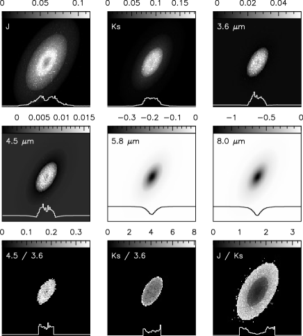
Figure 19: Model A simulation outputs for Taurus–Perseus region. Last row is ratio maps. The histogram displays the horizontal cut along the x axis through the center. Grey scale given in MJy sr^-1.

5 Conclusion

We explored a radiative transfer model in order to study the scattering of NIR and MIR light in dark clouds by varying the grain properties and evaluating the impact of other parameters such as the ISRF and the background field intensities. We confront our large sample of coreshine observations to the modeling and we selected a handful of cases to explore the capability of coreshine to disentangle dust properties. Our results are the following:

• The emergence of coreshine is a contrast issue which has to be treated carefully. The cloud background field estimation is a key point to the modeling. We adapted the Levenson method with careful flux conversion to the pertinent wavelengths. Moreover, the choice of keeping the standard ISRF is the safest approach and also a real challenge which will benefit from emission modeling in future studies.

• Merging previous samples of coreshine observations to build sufficient statistics, some Galactic regions appear to be favored. This could be considered in a big picture as the presence of previously grown grains in the initial diffuse medium of these individual regions. It opens the scope of modeling coreshine with regards to individual regions or for clouds in close environmental conditions (like L1517A,B,C,D or L134 and L183).

• The use of 3.6 and 4.5 $\mu$m coreshine bands and especially their ratio, referred to as coreshine ratio, brings additional constraints on the grain properties in the core.

• The highest coreshine ratios and fluxes are obtained for clouds which contain an embedded object, probing the influence of local change in the radiation field which has been tested qualitatively in our modeling.
  

Concerning the grain properties, the main conclusions are:

• Small grains have no influence in the modeling on the coreshine ratio.

• For any given coreshine ratio, the absolute 3.6 $\mu$m flux value is somewhat adjustable from both the cloud model and the phase function.

• The size increase is mandatory but not sufficient to explain coreshine. The coreshine ratio quantity tends to saturate with the grain size increase, both for spherical compact grains and for agglomerates of monomers. While bare spherical grains show a saturation of this ratio above a high exponential cut-off of 1 $\mu$m, fluffiness helps to raise the saturation limit.

• Since dust grains inside molecular clouds are expected to be icy, the role of ice mantles needs to be further investigated. Indeed, we expect ices to favor fluffiness and growth but in the meantime the only model we tested shows that it decreases the coreshine ratio. New models of icy grains are strongly needed.

• Both the NIR/MIR ratio for the core outer layer and the absence of emission at 5.8 $\mu$m for any layers eliminate a mix of silicates and carbonates that both include grains above $\sim$2 $\mu$m in meaningful quantity.

• Porosity has no impact at the studied wavelengths.

• The comparison with other wavelengths for a valid coreshine ratio can help to disentangle between the cloud models and the grain properties.

• In the case where the NIR and MIR do not sample the same zone, we might be able to peel the cloud layer by layer thanks to the multi-wavelength approach. If the same region is sampled then the grain size distribution properties have to be customized to be compatible with the observations at the different wavelengths.

In this paper, we constituted a database for the grain behavior covering grain growth by coagulation (up to 5 $\mu$m in size). We extended our study to aggregates and the presence of ice mantles and found several promising grain types which are able to reproduce the observations. We constrained the ISRF and the background value for different lines of sight and deduced the impact of the other free parameters on the modeling. The complementarity with NIR observations introduced to highlight the promising perspective of a 3D multi–wavelength cloud modeling has to be investigated on a real cloud following all the key points above and extending the study to far–IR emission.

Table 5: 3.6 $\mu$m coreshine intensity and 4.5/3.6 coreshine ratio sorted by increasing ratio value for each detected cloud of the four regions.

Name	3.6 $\mu$m intensity	4.5/3.6		Protostar	Class	LBol	refs
	kJy sr-1	median	FWHM			L☉
Taurus–Perseus
G171.80$-$09.78	10	–	–
CB24	15	–	–
L1503	22	–	–
G179.18$-$19.62	22	–	–
G182.19$-$17.71	23	–	–
G170.81$-$18.34	26	–	–
L1552	26	–	–
G169.82$-$19.39	27	–	–
CB20	27	–	–
G173.45$-$13.34	30	–	–
G177.89$-$20.16	33	–	–
B18–3 = G174.39$-$13.43	35	–
G154.68$-$15.34	49	0.35	0.10
G170.99$-$15.81	36	0.36	0.17
L1506C	33	0.37	0.26
L1507A (G171.51$-$10.59)	41	0.41	0.15
IRAS03282+3035	47	0.42	0.14	IRAS 03282+3035	Class 0	1.2	1
G173.69$-$15.55	32	0.43	0.10
L1544	39	0.43	0.32
L1512	30	0.44	0.31
L1521E	51	0.46	0.25
L1498	34	0.47	0.22
G171.34$-$10.67	58	0.47	0.20
G170.26$-$16.02	87	0.50	0.30	IRAS 04181+2654AB	Class I	–	2
L1521F	53	0.51	0.20	VeLLO	Class 0	0.36	3
L1517A	57	0.51	0.28
L1517B	43	0.51	0.28
G157.10$-$08.70	34	0.52	0.15	IRAS 03586+4112 (?)
L1517C	29	0.53	0.28
L1507	41	0.54	0.35	2MASS J04432023+2940060	Class II	–	4
IRAM04191	140	0.57	0.36	IRAM04191–IRS	Class 0	0.28	5
L1439	81	0.60	0.29	IRAS 04559+5200	Class I	$\geq$ 0.5	6,7
TMC2	100	0.64	0.47	IRAS 04294+2413	Class 0 ?	0.78 (LIR)	8
L1448mm	59	0.64	0.44	L1448-mm	Class 0	8.6	9
G163.21$-$08.40	67	0.64	0.46	IRAS 04218+3708 (?)
G157.12$-$11.56	390	0.64	0.39	IRAS 03484+3845 (?)
G155.45$-$14.59	210	0.64	0.27	IRAS 03330+3727 (?)
G160.51$-$16.84	61	0.66	0.51	B5 IRS1 (IRAS 03445+3242)	Class I	3.8	10
G171.91$-$15.65	310	0.77	0.39	DG Tau B	Class I	0.86	2,11
Barnard18–1	97	0.79	0.39	IRAS 04292+2422(E+W)	Class I	0.6	10
G163.32$-$08.42	63	0.82	0.30	IRAS 04223+3700	Class 1	2.7	10
G158.86$-$21.60	74	0.95	0.40	IRAS 03249+2957	Class I	0.3	1
Barnard1	100	1.1	0.51	IRAS 03301+3057 (cluster)	Class I	2.7 (LIR)	12
L183 / L134
L183	58	0.37	0.14
L134	$>$ 30	–	–
Chameleon
G302.89$-$14.05	16	–	–
G298.34$-$13.03	25	–	–
G303.28$-$13.32	25	–	–
Mu8	27	–	–
G297.09$-$16.02	39	0.35	0.23
G303.09$-$16.04	77	0.43	0.23
G303.68$-$15.32	21	0.44	0.23
G303.39$-$14.26	150	0.50	0.33	IRAS 12553$-$7651	Class I	1.2	13
G303.15$-$17.34	32	0.60	0.36
G303.72$-$14.86	100	0.74	0.52	IRAS 13014$-$7723	Class II	1.6	14,15
Cepheus
G093.20+09.53	18	–	–
L1155E	22	–	–
G093.16+09.61	24	–	–
G130.56+11.51	24	–	–
L1157	28	0.41	0.09	IRAS 20386+6751	Class 0	11	16
L1155C	29	0.44	0.17
L1247	110	0.46	0.36
L1251A	62	0.50	0.40	L1251A–IRS1–4	Class I, I, 0 & 0	IRS3 = 0.8	17
L1333	25	0.50	0.18
L1148	24	0.54	0.38	L1148–IRS	Class I	0.44	18
L1152	39	0.58	0.24	L1152 1–3	Class 0, I, & I	1.5, 0.6, 2.1	18
L1262	92	0.62	0.33	IRAS 23238+7401	Class 0	1.5	19
L1157–outflow	31	0.71	0.22	outflow shock region ?
L1228	110	0.73	0.50	IRAS 20582+7724 (cluster)	Class I	2.3	18
L1221	160	0.81	0.52	L1221–IRS1 & 3	Class 0 & 0	3.0 & 1.4	18
L1251C	260	0.81	0.59	IRAS 22343+7501 (cluster)	Class I	33	18
L1251B	160	0.89	0.57	IRAS 22376+7455 (cluster)	Class 0	15	18

Table 5: continued.

Appendix A Isotropy versus anisotropy for the incident radiation field

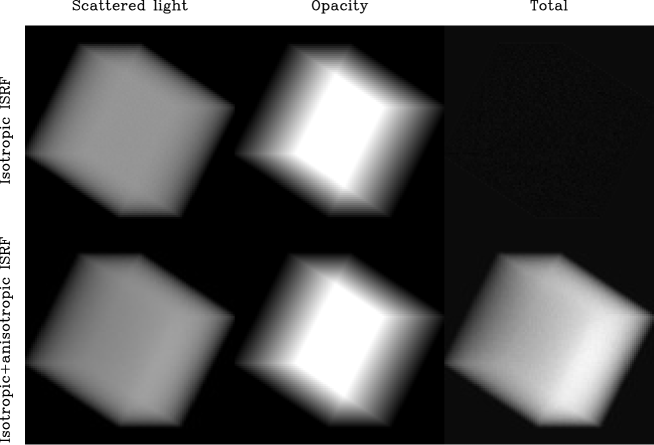
Figure 20: A cubic cloud filled with scattering (absorptionless) dust at constant density in an isotropic (upper row) or isotropic+anisotropic (lower row) field. The left column shows the scattered photons only, the middle column the opacity along the line of sight (identical for both cases) and the right column the net surface brightness.

Coreshine (and any kind of scattering processes) can be seen in emission only if it follows a number of conditions as discussed in Sect. 4.2. Another compulsory condition is the anisotropy of the incident ISRF. This anisotropy can come from large scales (like galactic structure) or small scales (like stars, near or far). To illustrate the importance of anisotropy we consider two simple cases: only isotropic illumination or the combination of one type of anisotropic source with the isotropic illumination.

If the ISRF is isotropic, there is no preferred direction for photons to travel. To see the cloud in emission, we need to introduce some anisotropy to concentrate photons towards a privileged direction, i.e. the observer. The cloud would therefore have to produce this anisotropy. To increase the number of photons towards the observer, the cloud would have to act like a telescope mirror pointed at the Earth to collect photons from a large number of directions to redirect them in a single direction (this would of course lower the number of photons scattered in some other directions). Since the cloud has no such focusing capabilities and the observer no privileged position, an isotropic ISRF cannot make a cloud glow. In fact, for any direction across the cloud there are as many deviated photons away from that line than photons from other directions being deviated into that propagation line and all the scatterings cancel out. This is in an ideal case without absorption. In presence of absorption, a part of the photons are lost and the cloud can only appear as a darker object against the background sky, never in emission. The field must therefore be anisotropic.

In the anisotropic case, there is one noticeable direction which is the line going from the localized light source to the cloud (we consider a single source of photons, like a nearby star, superimposed on an isotropic ISRF). This is the path with the highest number of photons traveling towards the cloud. Like in the isotropic case, photons enter from all directions and are partly deviated, partly untouched (and partly absorbed but we keep ignoring absorption here). The difference with the isotropic case is that along this particular line, across the cloud, there will be a larger number of deflected photons away from it than photons brought back onto it. The contrary can happen for some or all of the other directions (depending on details such as the phase function of the grain scattering properties). Therefore, away from this path, the number of deviated photons leaving the cloud is increasing (while they are decreasing along the path). Eventually, there can be more photons deviated towards the observer from the anisotropic source than photons coming from behind the cloud and deviated away from the observer. The net effect is to show the cloud in emission.

To illustrate this effect we ran a model based on a cube of constant density, tilted at 30° angles on two axes to see the edges and three sides. The cube is either in an isotropic field or a composite of isotropic and anisotropic fields. It is filled with dust with scattering capability only (absorption coefficient is set to zero). Figure 20 shows the results. The left column shows slightly different images of scattered photons but taking into account the background illumination absorption due to the cloud opacity (displayed in the central figure), following eq. 3, the cloud completely disappears in the isotropic field. This is explained by the fact that all the photons scattered towards the observer (as seen in the left panel) are exactly compensated by the photons scattered away from the line of sight for the radiation field coming from behind the cloud. A close inspection of the image reveals the cube by the numerical noise of the Monte Carlo radiative transfer code only. If the cloud opacity had not been set to zero, the cloud would have been seen in absorption against the background, while for the isotropic+anisotropic case, the cloud would have appeared in emission or in absorption depending on the balance (Sect. 4.2).

Appendix B Global method for stellar contribution subtraction.

We assume that the intensity in the DIRBE1 (1.25 $\mu$m) and DIRBE2 (2.2 $\mu$m) bands is only due to the sum of individual stellar contributions (PSC):

$$I_{K}=I^{*}_{K}=\sum I_{PSC,K}=DIRBE{2}$$ (7)

$$I_{J}=I^{*}_{J}=\sum I_{PSC,J}=DIRBE{1}.$$ (8)

The intrinsic color I_int of the stellar component has been measured from high galactic latitude and low dust emission regions and is also equal to:

$$I_{int}(\lambda_{1}/\lambda_{2})=\frac{I^{*}_{\lambda 2}\times exp(\tau_{\lambda 2})}{I^{*}_{\lambda 1}\times exp(\tau_{\lambda 1})}$$ (9)

We deduce the extinction on each line of sight by using the measured value of the intrinsic color between J and K ($I_{\mathrm{int}}(J/K)=1.$ ), its definition (eq. 9) and the previous assumptions (eq. 7 and 8):

$$I_{\mathrm{int}}(J/K)=1.=\frac{I^{*}_{K}\times exp(\tau_{K})}{I^{*}_{J}\times exp(\tau_{J})}=\frac{DIRBE{2}}{DIRBE{1}}\times exp(\tau_{K}-\tau_{J})$$ (10)

Finally we use eq. 9 to yield the stellar contribution in each band:

$$I^{*}_{3.6}=I_{int}(J/3.6)\times I^{*}_{J}\times exp(\tau_{J})/exp(\tau_{3.6})$$ (11)

Taking into account our assumption (eq. 8) and the conversion coefficient deduced from the extinction curve of Rieke & Lebofsky (1985) with R_V = 3.1 we obtain:

$$I^{*}_{3.6}=I_{int}(J/3.6)\times DIRBE{1}\times exp(\tau_{J})/exp(0.5\tau_{K})$$ (12)

$$I^{*}_{3.6}=I_{int}(J/3.6)\times DIRBE{1}\times\frac{DIRBE2}{DIRBE1}\times\frac{1.}{exp(0.5)}$$ (13)

$$I^{*}_{3.6}=I_{int}(J/K)\times I_{int}(K/3.4)\times DIRBE2\times\frac{1.}{exp(0.5)}$$ (14)

with I${}_{int}(J/K)$ = 1. and $I_{int}(3.4/K)=1.7$ (Bernard et al. 1994).

We obtain the diffuse emission map:

$$I_{\mathrm{diff}}(3.4)=DIRBE{3}-I^{*}_{3.4}$$ (15)

In the same way using $I_{\mathrm{int}}(4.9/3.4)=2.1$ we compute the other diffuse emission map:

$$I_{\mathrm{diff}}(4.9)=DIRBE{4}-I^{*}_{4.9}$$ (16)

Appendix C Source sample

Table 6: Source table classified region by region

Name	Gal. Longitude	Gal. Latitude	Status	Region
G190.15$-$14.34	$-$169.85	$-$14.34	P?	Orion
L1570	$-$169.32	$-$0.45	N	Orion
CB42	$-$167.42	$-$2.80	N	Orion
CB41	$-$167.30	$-$2.93	N	Orion
G195.09$-$16.41	$-$164.90	$-$16.41	C	Orion
G196.21$-$15.50	$-$163.78	$-$15.50	P	Orion
B35A	$-$163.07	$-$10.36	P	Orion
G198.03$-$15.24	$-$161.96	$-$15.25	P	Orion
CB46	$-$156.98	$-$3.73	C	Orion
G209.28$-$19.62	$-$150.71	$-$19.63	N	Orion
G214.69$-$19.94	$-$145.31	$-$19.95	C?	Orion
G203.57$-$30.08	$-$156.42	$-$30.09	N	Eridanus
G202.21$-$09.17	$-$157.79	$-$9.18	N	Monoceros
L1633	$-$153.13	$-$4.39	A	Monoceros
G211.70$-$12.17	$-$148.29	$-$12.18	N	Monoceros
G215.41$-$16.39	$-$144.58	$-$16.39	C	Monoceros
G216.69$-$13.88	$-$143.31	$-$13.88	C	Monoceros
G216.76$-$16.06	$-$143.24	$-$16.06	C	Monoceros
G219.28$-$09.27	$-$140.71	$-$9.27	U	Monoceros
G219.35$-$09.70	$-$140.65	$-$9.71	N	Monoceros
G219.37$-$07.68	$-$140.63	$-$7.69	N?	Monoceros
G219.26$-$17.89	$-$140.73	$-$17.90	C	Lepus
G227.30$-$03.77	$-$132.69	$-$3.77	N	Canis major
BHR7	$-$107.47	0.07	C	Gum/Vela
CG30/31	$-$106.82	$-$1.66	P	Gum/Vela
BHR13	$-$106.41	2.95	A	Gum/Vela
BHR14	$-$106.18	$-$10.91	P+C?	Gum/Vela
BHR16	$-$104.56	$-$3.95	C?	Gum/Vela
DC257.3$-$2.5	$-$102.72	$-$2.45	C?+A	Gum/Vela
BHR21	$-$100.56	$-$12.73	C+P	Gum/Vela
BHR22	$-$100.48	$-$16.45	P	Gum/Vela
BHR30	$-$94.73	$-$0.01	A	Gum/Vela
BHR31	$-$94.35	$-$7.69	A	Gum/Vela
DC266.0$-$7.5	$-$94.00	$-$7.41	A	Gum/Vela
BHR36	$-$92.64	$-$7.51	A	Gum/Vela
BHR37	$-$92.54	$-$7.41	A+P	Gum/Vela
BHR34	$-$92.42	$-$6.47	C?+P?	Gum/Vela
BHR40	$-$92.42	$-$6.44	P	Gum/Vela
BHR38/39	$-$92.36	$-$6.01	P	Gum/Vela
BHR41	$-$92.35	$-$7.36	A	Gum/Vela
BHR42	$-$92.04	$-$7.78	P	Gum/Vela
BHR44	$-$90.53	3.95	A	Gum/Vela
BHR43	$-$90.50	2.95	A	Gum/Vela
BHR47	$-$87.55	2.01	A	Gum/Vela
BHR53	$-$85.78	$-$0.39	A	Gum/Vela
BHR55	$-$84.00	1.85	A	Gum/Vela
BHR56	$-$83.81	$-$10.59	C	Gum/Vela
BHR59	$-$68.94	$-$1.66	A	Carina
BHR71	$-$62.28	$-$2.78	A	Musca
DC298.3$-$131 (G298.34$-$13.03)	$-$61.66	$-$13.04	C	Musca
BHR76	$-$59.42	$-$3.13	N	Musca
Mu8	$-$58.78	$-$8.28	C	Musca
BHR78	$-$58.78	$-$0.37	A	Crux
BHR83	$-$57.90	7.44	C	Centaurus
G295.13$-$17.56	$-$64.86	$-$17.56	N	Chamaleon
G297.09$-$16.02	$-$62.91	$-$16.02	C	Chamaleon
G302.89$-$14.05	$-$57.11	$-$14.05	C?	Chamaleon
G303.09$-$16.04	$-$56.91	$-$16.04	C	Chamaleon
G303.15$-$17.34	$-$56.84	$-$17.35	C	Chamaleon
G303.28$-$13.32	$-$56.71	$-$13.32	C?	Chamaleon
G303.39$-$14.26	$-$56.60	$-$14.27	C	Chamaleon
G303.68$-$15.32	$-$56.32	$-$15.33	C	Chamaleon
G303.72$-$14.86	$-$56.27	$-$14.86	C	Chamaleon
BHR86	$-$56.13	$-$14.16	U	Chamaleon
DC338.2+16.4	$-$21.84	16.38	C	Lupus
DC338.8+16.5$-$2	$-$20.97	16.73	C	Lupus
L1681 ($ρ$ Oph E)	$-$7.00	16.65	C	$\rho$ Oph
$ρ$ Oph D	$-$6.35	17.71	N	$\rho$ Oph
G354.19+16.27	$-$5.80	16.28	C	$\rho$ Oph
$ρ$ Oph 9	$-$5.63	16.17	C+P+A	$\rho$ Oph
G356.96+07.27	$-$3.03	7.27	N	$\rho$ Oph
B59	$-$2.89	7.12	C	$\rho$ Oph
L1772	$-$1.30	6.03	U	$\rho$ Oph
L4	0.24	11.71	C	$\rho$ Oph
L43	1.35	20.98	C	$\rho$ Oph
B68	1.52	7.08	N	$\rho$ Oph
Fest 1-457	1.71	3.651	N	$\rho$ Oph
B72	1.78	6.95	N	$\rho$ Oph
L63	1.84	16.59	C	$\rho$ Oph
L100 (G003.07+09.95)	3.08	9.97	U	$\rho$ Oph
L111	3.30	10.43	C	$\rho$ Oph
CB68	4.51	16.34	C	$\rho$ Oph
L158	4.86	19.62	N	$\rho$ Oph
G004.92+17.95	4.92	17.95	?	$\rho$ Oph
L162 (G005.03+19.07)	5.03	19.08	N	$\rho$ Oph
L173	5.30	11.08	C	$\rho$ Oph
L191 (G006.08+20.26)	6.09	20.26	N	$\rho$ Oph
L204C$-$2 (in G006.41+20.56)	6.34	20.46	P + C?	$\rho$ Oph
G006.41+20.56 (core$-$s4)	6.42	20.56	C	$\rho$ Oph
L234E	7.65	21.18	P	$\rho$ Oph
L260 (G008.67+22.14 )	8.68	22.14	C	$\rho$ Oph
L328	13.03	$-$0.83	A	$\rho$ Oph?
CB103	23.89	11.12	C	$\rho$ Oph
L723	52.98	3.05	A/N	$\rho$ Oph
L1780	$-$1.10	36.88	P	Serpens
L134A	4.24	35.81	C	Serpens
L183 (G006.04+36.74)	6.00	36.74	C	Serpens
G011.40+36.19	11.40	36.19	N	Serpens
L429$-$C	21.62	3.75	A	Serpens
L438	22.29	4.97	N	Serpens
L462$-$1	23.69	7.56	N	Serpens
L483	24.89	5.40	A	Serpens
L492	25.50	6.18	C	Serpens
L507	26.72	6.71	N	Serpens
L648$-$1(G043.02+08.36)	43.02	8.37	C	Hercules
L531	28.46	$-$6.41	C	Aquila
G032.93+02.68	32.94	2.69	A	Aquila
B335	44.94	$-$6.56	C	Aquila
L673	46.28	$-$1.25	A	Aquila
L673$-$7	46.46	$-$1.46	A	Aquila
L675	46.52	$-$2.02	A	Aquila
CB188	46.53	$-$1.01	A	Aquila
L694$-$2	48.41	$-$5.83	C	Aquila
L771(G057.08+04.46)	57.10	4.45	N	Vulpecula
G089.03$-$41.28	89.03	$-$41.29	N	Pegasus
B158	89.64	$-$6.63	C	Cygnus
G092.26+03.80	92.26	3.81	A	Cygnus
L1014	92.57	$-$0.25	N	Cygnus
L1021	93.00	0.71	N	Cygnus
G093.16+09.61	93.16	9.61	C	Cygnus
G093.20+09.53	93.21	9.54	C	Cygnus
G093.22$-$04.59	93.23	$-$4.59	P?	Cygnus
G093.31$-$11.68	93.32	$-$11.68	N	Lacerta
CB228	93.89	7.60	C	Cepheus
B148	96.31	10.02	C	Cepheus
L1148	102.18	15.26	C	Cepheus
L1155E	102.61	15.20	C	Cepheus
L1155C$-$2	102.70	15.37	C	Cepheus
L1165	103.17	2.68	N	Cepheus
L1166	103.29	3.18	N	Cepheus
G105.55+10.40	105.56	10.41	N	Cepheus
L1197	106.35	0.48	N	Cepheus
G108.23+15.61	108.24	15.62	N?	Cepheus
L1221	110.65	9.64	C	Cepheus
L1228	111.67	20.22	C	Cepheus
Bern48	112.40	20.59	U	Cepheus
L1251A$-$2	113.99	14.92	C	Cepheus
L1251A	114.19	14.81	C	Cepheus
L1251C	114.48	14.69	C	Cepheus
L1251B	114.68	14.48	C	Cepheus
L1262	117.12	12.41	C	Cepheus
L1247	125.42	12.41	C	Cepheus
G128.25+20.78	128.25	20.78	U	Cepheus
L1152	102.36	15.98	C	Draco
L1157	102.65	15.80	C	Draco
G108.85$-$00.80	108.85	$-$0.80	P	Cas
L1253	115.84	$-$3.54	N	Cas
L1301	122.09	$-$0.36	A	Cas
CB6	122.60	5.00	P?	Cas
L1325	127.27	0.55	A	Cas
G127.88+02.66	127.88	2.67	?	Cas
L1333	128.89	13.69	C	Cas
G128.95$-$00.18	128.96	$-$0.19	A+P	Cas
L1345	130.36	0.77	N	Cas
G130.56+11.51	130.56	11.51	C	Cas
L1355	133.55	8.61	N	Cas
G131.35$-$45.73	131.36	$-$45.73	N	Pisces
G145.87+17.77	145.88	17.78	C	Cameleopardalis
L1389	147.02	3.39	C	Cameleopardalis
G149.41+03.37	149.41	3.38	A?	Cameleopardalis
G149.58+03.45	149.59	3.45	P	Cameleopardalis
G150.22+03.91	150.23	3.92	C	Cameleopardalis
G151.45+03.95	151.46	3.96	P?	Cameleopardalis
CB24	155.76	5.91	C	Auriga
L1439	156.05	6.02	C	Auriga
G159.65+11.39	159.65	11.40	N?	Auriga
G170.77$-$08.51	170.77	$-$8.52	U	Auriga
L1512	171.86	$-$5.24	C	Auriga
L1517	172.38	$-$8.09	C	Auriga
L1448	158.06	$-$21.42	C	Aries
L1455 (G158.86$-$21.60)	158.86	$-$21.60	C	Aries
L1457 (G158.88$-$34.18)	158.88	$-$34.18	C	Aries
G158.97$-$33.01	158.97	$-$33.02	C	Aries
IRAS03282+3035	159.09	$-$20.66	C	Aries
G159.67$-$34.31	159.68	$-$34.32	N?	Aries
G154.68$-$15.34	154.69	$-$15.35	C	Perseus
G155.45$-$14.59	155.46	$-$14.59	C?	Perseus
G157.10$-$08.70	157.10	$-$8.71	C	Perseus
G157.12$-$11.56	157.13	$-$11.57	C	Perseus
Barnard1	159.20	$-$20.12	C	Perseus
B5 (G160.51$-$16.84)	160.51	$-$16.84	C	Perseus
G162.90$-$08.63	162.91	$-$8.63	N	Perseus
G163.21$-$08.40	163.21	$-$8.40	C?	Perseus
G163.32$-$08.42	163.32	$-$8.42	C	Perseus
G169.82$-$19.39	169.83	$-$19.39	C	Taurus
L1498	169.97	$-$19.00	C	Taurus
G170.26$-$16.02	170.27	$-$16.02	C	Taurus
G170.81$-$18.34	170.82	$-$18.35	C?	Taurus
L1521B$-$2(G170.99$-$15.81)	170.87	$-$15.87	C	Taurus
L1503	170.92	$-$10.93	C	Taurus
L1506C	171.15	$-$17.57	C	Taurus
L1507A (G171.51$-$10.59)	171.34	$-$10.70	C	Taurus
G171.34$-$10.67	171.34	$-$10.67	C	Taurus
L1521F (G171.49$-$14.908)	171.49	$-$14.90	C	Taurus
CB23	171.50	$-$10.60	C	Taurus
L1521$-$2	171.55	$-$14.67	U	Taurus
G171.80$-$09.78	171.80	$-$9.78	C	Taurus
G171.91$-$15.65	171.91	$-$15.66	C?	Taurus
L1521E	172.09	$-$15.20	C	Taurus
G173.45$-$13.34	173.45	$-$13.34	C	Taurus
L1524$-$4	173.62	$-$16.26	C	Taurus
B18$-$2 (G173.69$-$15.55)	173.66	$-$15.54	C	Taurus
B18$-$1	173.82	$-$15.87	C	Taurus
TMC2	174.06	$-$15.81	C	Taurus
G174.08$-$13.24	174.09	$-$13.25	C?	Taurus
CB20	174.31	$-$15.01	C	Taurus
B18$-$3 (G174.44$-$15.75)	174.45	$-$15.74	C	Taurus
G174.50$-$19.88	174.51	$-$19.89	P	Taurus
B18$-$5	174.72	$-$15.44	U	Taurus
G177.89$-$20.16	177.89	$-$20.16	C	Taurus
L1544	177.98	$-$9.71	C	Taurus
L1552	179.02	$-$6.75	C	Taurus
G179.18$-$19.62	179.19	$-$19.63	C?	Taurus
IRAM04191	179.56	$-$23.50	C	Taurus
G182.19$-$17.71	182.20	$-$17.72	C	Taurus

Table 6: continued.

References

- Alcalá et al. (2008) Alcalá, J. M., Spezzi, L., Chapman, N., et al. 2008, ApJ, 676, 427
- Anderl et al. (2013) Anderl, S., Guillet, V., Pineau des Forêts, G., & Flower, D. R. 2013, A&A, 556, A69
- Andersen et al. (2013) Andersen, M., Steinacker, J., Thi, W.-F., et al. 2013, A&A, 559, A60
- André et al. (2000) André, P., Ward-Thompson, D., & Barsony, M. 2000, Protostars and Planets IV, 59
- Ascenso et al. (2012) Ascenso, J., Lada, C. J., Alves, J., Román-Zúñiga, C. G., & Lombardi, M. 2012, arXiv.org, 6556
- Benjamin et al. (2003) Benjamin, R. A., Churchwell, E., Babler, B. L., et al. 2003, PASP, 115, 953
- Bernard et al. (1994) Bernard, J. P., Boulanger, F., Désert, F.-X., et al. 1994, A&A, 291, L5
- Bertin & Arnouts (1996) Bertin, E. & Arnouts, S. 1996, A&AS, 117, 393
- Bonnarel et al. (2000) Bonnarel, F., Fernique, P., Bienaymé, O., et al. 2000, A&AS, 143, 33
- Brady Ford & Shirley (2011) Brady Ford, A. & Shirley, Y. L. 2011, ApJ, 728, 144
- Chapman et al. (2013) Chapman, N. L., Davidson, J. A., Goldsmith, P. F., et al. 2013, ApJ, 770, 151
- Chapman et al. (2009) Chapman, N. L., Mundy, L. G., Lai, S.-P., & Evans, II, N. J. 2009, ApJ, 690, 496
- Chen et al. (2012) Chen, X., Arce, H. G., Dunham, M. M., & Zhang, Q. 2012, The Astrophysical Journal, 747, L43
- Cohen et al. (2003) Cohen, M., Wheaton, W. A., & Megeath, S. T. 2003, AJ, 126, 1090
- Compiègne et al. (2011) Compiègne, M., Verstraete, L., Jones, A. P., et al. 2011, A&A, 525, 103
- Connelley & Greene (2010) Connelley, M. S. & Greene, T. P. 2010, AJ, 140, 1214
- Cutri et al. (2012a) Cutri, R. M., Skrutskie, M. F., van Dyk, S., et al. 2012a, VizieR Online Data Catalog, 2311, 0
- Cutri et al. (2012b) Cutri, R. M., Wright, E. L., Conrow, T., et al. 2012b, Explanatory Supplement to the WISE All-Sky Data Release Products, Tech. rep.
- Di Francesco et al. (2008) Di Francesco, J., Johnstone, D., Kirk, H., MacKenzie, T., & Ledwosinska, E. 2008, ApJS, 175, 277
- Doty et al. (2005) Doty, S. D., Everett, S. E., Shirley, Y. L., Evans, N. J., & Palotti, M. L. 2005, Monthly Notices of the Royal Astronomical Society, 359, 228
- Dunham et al. (2008) Dunham, M. M., Crapsi, A., Evans II, N. J., et al. 2008, ApJS, 179, 249
- Dunham et al. (2006) Dunham, M. M., Evans, II, N. J., Bourke, T. L., et al. 2006, ApJ, 651, 945
- Enoch et al. (2009) Enoch, M. L., II, N. J. E., Sargent, A. I., & Glenn, J. 2009, The Astrophysical Journal, 692, 973
- Evans et al. (2009) Evans, N. J. I., Dunham, M. M., Jørgensen, J. K., et al. 2009, The Astrophysical Journal Supplement, 181, 321
- Evans et al. (2001) Evans, N. J. I., Rawlings, J. M. C., Shirley, Y. L., & Mundy, L. G. 2001, The Astrophysical Journal, 557, 193
- Fazio et al. (2004) Fazio, G. G., Hora, J. L., Allen, L. E., et al. 2004, ApJS, 154, 10
- Fitzpatrick & Massa (2007) Fitzpatrick, E. L. & Massa, D. 2007, ApJ, 663, 320
- Flagey et al. (2006) Flagey, N., Boulanger, F., Verstraete, L., et al. 2006, A&A, 453, 969
- Fraser et al. (2001) Fraser, H. J., Collings, M. P., McCoustra, M. R. S., & Williams, D. A. 2001, MNRAS, 327, 1165
- Gómez-Ruiz et al. (2013) Gómez-Ruiz, A. I., Hirano, N., Leurini, S., & Liu, S.-Y. 2013, A&A, 558, A94
- Gorjian et al. (2000) Gorjian, V., Wright, E. L., & Chary, R. R. 2000, ApJ, 536, 550
- Górski et al. (2005) Górski, K. M., Hivon, E., Banday, A. J., et al. 2005, ApJ, 622, 759
- Green et al. (2013) Green, J. D., Evans, II, N. J., Jørgensen, J. K., et al. 2013, ApJ, 770, 123
- Habing (1968) Habing, H. J. 1968, Bull. Astron. Inst. Netherlands, 19, 421
- Hauser et al. (1998) Hauser, M. G., Arendt, R. G., Kelsall, T., et al. 1998, ApJ, 508, 25
- Hirashita (2012) Hirashita, H. 2012, MNRAS, 422, 1263
- Hirashita & Voshchinnikov (2014) Hirashita, H. & Voshchinnikov, N. V. 2014, MNRAS, 437, 1636
- Jarrett et al. (2011) Jarrett, T. H., Cohen, M., Masci, F., et al. 2011, ApJ, 735, 112
- Jones (2013) Jones, A. P. 2013, A&A, 555, A39
- Jones & Cohen (1986) Jones, B. F. & Cohen, M. 1986, ApJ, 311, L23
- Juvela (2005) Juvela, M. 2005, A&A, 440, 531
- Juvela et al. (2012) Juvela, M., Malinen, J., & Lunttila, T. 2012, A&A, 544, A141
- Juvela & Padoan (2003) Juvela, M. & Padoan, P. 2003, A&A, 397, 201
- Kirk et al. (2009) Kirk, J. M., Ward-Thompson, D., Di Francesco, J., et al. 2009, ApJS, 185, 198
- Kristensen et al. (2012) Kristensen, L. E., van Dishoeck, E. F., Bergin, E. A., et al. 2012, A&A, 542, A8
- Lallement et al. (2014) Lallement, R., Vergely, J.-L., Valette, B., et al. 2014, A&A, 561, A91
- Lawrence & Keene (2004) Lawrence, C. & Keene, J. 2004, Spitzer Proposal, 94
- Lee et al. (2010) Lee, J.-E., Lee, H.-G., Shinn, J.-H., et al. 2010, ApJ, 709, L74
- Lehtinen & Mattila (1996) Lehtinen, K. & Mattila, K. 1996, A&A, 309, 570
- Levenson et al. (2007) Levenson, L. R., Wright, E. L., & Johnson, B. D. 2007, ApJ, 666, 34
- Li & Draine (2001) Li, A. & Draine, B. T. 2001, ApJ, 554, 778
- Lippok et al. (2013) Lippok, N., Launhardt, R., Semenov, D., et al. 2013, A&A, 560, A41
- Luhman et al. (2010) Luhman, K. L., Allen, P. R., Espaillat, C., Hartmann, L., & Calvet, N. 2010, ApJS, 186, 111
- Malinen et al. (2014) Malinen, J., Juvela, M., Zahorecz, S., et al. 2014, A&A, 563, A125
- Marshall et al. (2006) Marshall, D. J., Robin, A. C., Reylé, C., Schultheis, M., & Picaud, S. 2006, A&A, 453, 635
- Mathis et al. (1983) Mathis, J. S., Mezger, P. G., & Panagia, N. 1983, A&A, 128, 212
- Mattila (1970) Mattila, K. 1970, A&A, 9, 53
- McClure (2009) McClure, M. 2009, ApJ, 693, L81
- Min et al. (2006) Min, M., Dominik, C., Hovenier, J. W., de Koter, A., & Waters, L. B. F. M. 2006, A&A, 445, 1005
- Ochsenbein et al. (2000) Ochsenbein, F., Bauer, P., & Marcout, J. 2000, A&AS, 143, 23
- Onishi et al. (1998) Onishi, T., Mizuno, A., Kawamura, A., Ogawa, H., & Fukui, Y. 1998, ApJ, 502, 296
- Ormel et al. (2009) Ormel, C. W., Paszun, D., Dominik, C., & Tielens, A. G. G. M. 2009, Astronomy and Astrophysics, 502, 845
- Ossenkopf (1993) Ossenkopf, V. 1993, A&A, 280, 617
- Pagani et al. (2012) Pagani, L., Lefèvre, C., Bacmann, A., & Steinacker, J. 2012, A&A, 541, 154
- Pagani et al. (2010) Pagani, L., Steinacker, J., Bacmann, A., Stutz, A., & Henning, T. 2010, Science, 329, 1622
- Rebull et al. (2010) Rebull, L. M., Padgett, D. L., McCabe, C.-E., et al. 2010, ApJS, 186, 259
- Rieke & Lebofsky (1985) Rieke, G. H. & Lebofsky, M. J. 1985, ApJ, 288, 618
- Robitaille et al. (2007) Robitaille, T. P., Whitney, B. A., Indebetouw, R., & Wood, K. 2007, The Astrophysical Journal Supplement Series, 169, 328
- Roy et al. (2014) Roy, A., André, P., Palmeirim, P., et al. 2014, A&A, 562, A138
- Skrutskie et al. (2006) Skrutskie, M. F., Cutri, R. M., Stiening, R., et al. 2006, AJ, 131, 1163
- Spezzi et al. (2008) Spezzi, L., Alcalá, J. M., Covino, E., et al. 2008, ApJ, 680, 1295
- Stecklum et al. (2004) Stecklum, B., Launhardt, R., Fischer, O., et al. 2004, ApJ, 617, 418
- Steinacker et al. (2014a) Steinacker, J., Andersen, M., Thi, W.-F., & Bacmann, A. 2014a, A&A, 563, A106
- Steinacker et al. (2013) Steinacker, J., Baes, M., & Gordon, K. D. 2013, ARA&A, 51, 63
- Steinacker et al. (2014b) Steinacker, J., Ormel, C. W., Andersen, M., & Bacmann, A. 2014b, A&A, 564, A96
- Steinacker et al. (2010) Steinacker, J., Pagani, L., Bacmann, A., & Guieu, S. 2010, Astronomy and Astrophysics, 511, 9
- Stutz et al. (2010) Stutz, A. M., Launhardt, R., Linz, H., et al. 2010, A&A, 518, L87
- Tafalla & Santiago (2004) Tafalla, M. & Santiago, J. 2004, A&A, 414, L53
- van der Tak et al. (2013) van der Tak, F. F. S., Chavarría, L., Herpin, F., et al. 2013, A&A, 554, A83
- Walawender et al. (2005) Walawender, J., Bally, J., Kirk, H., & Johnstone, D. 2005, AJ, 130, 1795
- Walmsley et al. (2004) Walmsley, C. M., Flower, D. R., & Pineau des Forêts, G. 2004, A&A, 418, 1035
- Weingartner & Draine (2001) Weingartner, J. C. & Draine, B. T. 2001, ApJ, 548, 296
- Whittet et al. (2001) Whittet, D. C. B., Gerakines, P. A., Hough, J. H., & Shenoy, S. S. 2001, The Astrophysical Journal, 547, 872
- Whittet et al. (2013) Whittet, D. C. B., Poteet, C. A., Chiar, J. E., et al. 2013, ApJ, 774, 102
- Whitworth & Ward-Thompson (2001) Whitworth, A. P. & Ward-Thompson, D. 2001, ApJ, 547, 317
- Wright et al. (2010) Wright, E. L., Eisenhardt, P. R. M., Mainzer, A. K., et al. 2010, AJ, 140, 1868
- Ysard et al. (2013) Ysard, N., Abergel, A., Ristorcelli, I., et al. 2013, A&A, 559, A133
- Ysard et al. (2012) Ysard, N., Juvela, M., Demyk, K., et al. 2012, A&A, 542, A21
- Yusef-Zadeh et al. (1984) Yusef-Zadeh, F., Morris, M., & White, R. L. 1984, ApJ, 278, 186