$L_{2}$ Differentiability of Generalized Linear Models

Abstract

We derive conditions for $L_{2}$ differentiability of generalized linear models with error distributions not necessarily belonging to exponential families, covering both cases of stochastic and deterministic regressors. These conditions induce smoothness and integrability conditions for corresponding GLM-based time series models.

Keywords

Generalized linear models; $L_{2}$-differentiability; shape scale model; time series model for shape

Subclass

MSC 62F12, 62F35

1 Motivation

Introduced by Nelder and Wedderburn (1972), generalized linear models (GLMs) have become one of the most frequently used statistical models with a vast amount of published results. Hence, trying to give a full account on relevant literature would be pretentious. We instead refer to the monographs McCullagh and Nelder (1989) and Fahrmeir and Tutz (2001). When it comes to regularity assumptions, though, this literature focuses on GLMs which are exponential families, compare Haberman (1974, 1977); Fahrmeir (1990); Fahrmeir and Kaufmann (1985), or uses quasi-likelihood or pseudo-likelihood techniques to account for over/under-dispersion effects, seeGouriéroux et al. (1984); Nelder and Pregibon (1987); McCullagh and Nelder (1989). In some situations, exponential families are a too narrow class, though: E.g., recently log-linear models for generalized Pareto distributions have found applications in operational risk (compare Dahen and Georges (2010)), but distributions of extreme value type with unknown shape parameter do not fall into the range of exponential families and so far are not yet covered.

Heading for asymptotic results and robustness, we are not only interested in consistency results for specific estimators like maximum likelihood estimators (MLEs), but rather in local asymptotic normality (LAN) in the sense of Le​ Cam (1970); Hájek (1972). With the LAN property at hand a very powerful asymptotic framework as pioneered by Le​ Cam is available: It gives a precise setup in which to obtain strong optimality results for (estimators behaving asymptotically like) the MLE, i.e., the Asymptotic Convolution Theorem and the Asymptotic Minimax Theorem, see, e.g. Rieder (1994, Thms. 3.2.3 & 3.3.8) or van der Vaart (1998, Thms. 8.8 & 8.11). The LAN property entails necessary expansions for asymptotic maximin tests with explicit terms for the asymptotic maximin power under local alternatives (Le​ Cam, 1986, Sec.11.9); it is the starting point for efficient and adaptive estimation in semiparametric models (compare Bickel et al. (1993)) and for a comprehensive theory of optimally-robust procedures (see Rieder (1994, Chs. 5 & 7)).

Now, a sufficient condition for the LAN property is given by $L_{2}$-differentiability (see, e.g. Rieder (1994, Thm. 2.3.5)), and—at least in the i.i.d. setting—this is a necessary condition, too, compare Le​ Cam and Young (2000, Ch. 7, Prop. 3). Hence in this light, deriving smoothness of the model in terms of $L_{2}$-differentiability would be a desirable goal; i.e., to consider GLMs as particular parametric models and to derive their $L_{2}$-differentiability. For GLMs which are exponential families, this has already been achieved in Schlather (1994). Typically, however, scale-shape families as e.g. the generalized Pareto distributions are non-exponential. In this article, we hence generalize results of Rieder (1994, Sec. 2.4) on $L_{2}$-differentiability for linear regression models to also cover error distributions with a $k$-dimensional parameter and with regressors of possibly different length for each parameter. More specifically, we separately treat the case of stochastic regressors, which is of particular interest for incorporating (space-)time dependence, and of deterministic regressors as occurring in planned experiments.

While in principle $L_{2}$-differentiability of these models could be settled by general auxiliary results from Hájek (1972, Lem. A.1–A.3), or be placed in the framework of Rieder and Ruckdeschel (2001), our goal are sufficient conditions directly exploiting the regression structure. More specifically, these conditions refer to (i) smoothness of the error distribution model, (ii) (uniform) integrability of the scores ($L_{2}$-derivative) and (iii) suitably integrated continuity of the Fisher information of again the error distribution model.

At first glance, this might look like a technical exercise but setting up time series models where time-dependence is captured by a GLM-type link with (functions of) the own past observations as regressors, conditions (ii) and (iii) reveal to which extent the current error distribution may depend upon the past without making it “over-informative” for the present. More precisely, letting aside dimensionalities of the parameter of the error distribution and the regressors, the scores function of a GLM ${\cal P}$ with errors from a distribution model ${\cal Q}$, link function $\ell$ and regressor $x$ is of form $\Lambda^{\cal P}_{\beta}(x,y)=\Lambda_{\ell(x\beta)}^{\cal Q}(y)\dot{\ell}(x\beta)x$, where $\Lambda^{\cal Q}_{\vartheta}$ are the parametric scores from model ${\cal Q}$. Now even if ${\cal Q}$ has fat tails and non-existing moments, in many cases $\Lambda^{\cal Q}_{\vartheta}$ still is square integrable, see e.g. the case of $\alpha$-stable distributions as in DuMouchel (1973) or the generalized extreme value and Pareto distributions GEVD and GPD explicated later on in this paper. If however, as in a autoregressive (AR) time series context with identity link $\ell(\theta)=\theta$, $x$ comes again from a distribution within ${\cal Q}$, the LAN property may fail due to a lack of integrability. This is the case in Andrews et al. (2009, Thm. 3.3), where in addition the authors obtain slower convergence rates for $\beta$ in an AR-model with $\alpha$-stable errors. One way to preserve the LAN property could consist in using a suitable link function $\ell$ such that the product $\dot{\ell}x$ becomes square integrable—see later in this paper for corresponding GPD and GEVD time series. This technique can be seen as an alternative / an extension to the approach using regression ranks as in Hallin et al. (2011), which in the respective case of a regression model with $\alpha$-stable errors and deterministic regressors achieves the same goal, i.e., extending the availabilty of the LAN property.

In this paper, we explicate the respective conditions (i)–(iii) for the cases of stochastic and deterministic regressors, respectively, in examples including—for reference and comparison—linear regression, Poisson, and Binomial regression, as well as scale-shape regression for the GPD and GEVD.

In particular for the latter distributions we give conditions which render a corresponding time series model accessible to the LAN type framework and thus contribute a new sort of GLM for extreme value type distributions where the tail weight respectively, the shape parameter depends on past observations in an autoregressive way. Thus, large extreme observations may foster or dampen the occurrence of future large extreme observations and controlling the extremal index (see Embrechts et al. (1997, p.413–423)) this way.

The rest of the paper is organized as follows: Section 2 provides the mathematical setup and the main results with Theorem 2.3 (for random carriers) and Theorem 2.6 (for deterministic carriers). The examples are worked out in Section 3. The proofs of our assertions are given in the appendix.

2 Main Results

Let $(\Omega,{\cal A})$ be a measurable space and ${\cal M}_{1}({\cal A})$ the set of all probability measures on ${\cal A}$. Consider $\mathcal{Q}=\{Q_{\vartheta}|\vartheta\in\Theta\}\subset{\cal M}_{1}({\cal A})$ a parametric model with open parameter domain $\Theta\subset\mathbb{R}^{k}$. Following Le​ Cam and Rieder, we write $dQ_{\vartheta}$ for the densities w.r.t. some dominating measure $\nu$ on ${\cal A}$ and denote the norm in the respective $L_{2}(\nu)$ space by $\|\,\cdot\|_{\mathcal{L}_{2}}$; as usual, $\nu$ is suppressed from notation as the choice of $\nu$ has no effect on respective convergence assertions. In this context, $L_{2}$ differentiability in the case of i.i.d. observations is defined as follows.

Definition 2.1

Model $\mathcal{Q}$ is called $L_{2}$ differentiable at $\vartheta\in\Theta$ if there exists a function $\Lambda^{\scriptscriptstyle\mathcal{Q}}_{\vartheta}\in L_{2}^{k}(P_{\vartheta})$ such that, as $h\rightarrow 0\in\mathbb{R}^{k}$

$$\left\|\sqrt{dQ_{\vartheta+h}}-\sqrt{dQ_{\vartheta}}\big{(}1+\tfrac{1}{2}(\Lambda^{\scriptscriptstyle\mathcal{Q}}_{\vartheta})^{\scriptscriptstyle\;\textrm{T}}h\big{)}\right\|_{\mathcal{L}_{2}}=\mathop{\rm{{}o{}}}\nolimits(|h|).$$ (2.1)

Then, $\Lambda^{\scriptscriptstyle\mathcal{Q}}_{\vartheta}$ is the $L_{2}$ derivative and the $k\times k$ matrix $\mathcal{I}^{\scriptscriptstyle\mathcal{Q}}_{\vartheta}=\mathop{\rm{{}E{}}}\nolimits_{\vartheta}\Lambda^{\scriptscriptstyle\mathcal{Q}}_{\vartheta}(\Lambda^{\scriptscriptstyle\mathcal{Q}}_{\vartheta})^{\scriptscriptstyle\;\textrm{T}}$ is the Fisher information of $\mathcal{Q}$ at $\vartheta$.
We say that $\mathcal{Q}$ is continuously $L_{2}$ differentiable at $\vartheta$ if, for any $h\to 0\in\mathbb{R}^{k}$,

$$\sup_{t\in{\scriptstyle\mathbb{R}}^{k}\colon\,|t|\leq 1}\left\|\sqrt{dQ_{\vartheta+h}}(\Lambda^{\scriptscriptstyle\mathcal{Q}}_{\vartheta+h})^{\scriptscriptstyle\;\textrm{T}}t-\sqrt{dQ_{\vartheta}}(\Lambda^{\scriptscriptstyle\mathcal{Q}}_{\vartheta})^{\scriptscriptstyle\;\textrm{T}}t\right\|_{\mathcal{L}_{2}}=\mathop{\rm{{}o{}}}\nolimits(1).$$ (2.2)

Introducing regressors to explain parameter $\vartheta$, we turn model $\mathcal{Q}$ into a regression model $\mathcal{P}$ with parameter $\beta$. To this end, for $p\in\mathbb{N}$, let $\pi\in\mathbb{N}^{k}$, $\pi=(p_{h})_{h=1,\ldots,k}$ be a partition of the $p$ coordinates into blocks of dimension $p_{h}$, i.e., $\sum_{h}p_{h}=p$. Obviously, then each $x\in\mathbb{R}^{p}$ can unambiguously be indexed by the double index $(x_{h,j})_{{{h=1,\ldots,k}\atop{j=1,\ldots,p_{h}}}}$. For these blocks we define the following operators:

$$T_{\pi}\colon\mathbb{R}^{p}\times\mathbb{R}^{p}\to\mathbb{R}^{k},\quad(a,b)\mapsto T_{\pi}(a,b)=:a^{{\scriptscriptstyle\;\textrm{T}_{\scriptscriptstyle\pi}}}b=(\sum_{j=1}^{p_{h}}a_{h,j}b_{h,j})_{h=1,\ldots,k}$$ (2.3)

$$\rho_{\pi}\colon\mathbb{R}^{k}\times\mathbb{R}^{p}\to\mathbb{R}^{p},\quad(c,a)\mapsto\rho_{\pi}(c,a)=:c\,{\,{\cdot_{\scriptscriptstyle\pi}}\,}\,a=(c_{h}a_{h,j})_{{{h=1,\ldots,k}\atop{j=1,\ldots,p_{h}}}}$$ (2.4)

$$M_{\pi}\colon\mathbb{R}^{k\times k}\times\mathbb{R}^{p}\times\mathbb{R}^{p}\to\mathbb{R}^{p\times p},\quad(C,a,b)\mapsto M_{\pi}(C,a,b)=$$

$$\mbox{\hskip 170.71652pt}(C_{h_{1},h_{2}}a_{h_{1},j_{1}}b_{h_{2},j_{2}})_{{{h_{1},h_{2}=1,\ldots,k}\atop{j_{1},j_{2}=1,\ldots,p_{h}}}}.$$ (2.5)

We also write $C{\,{\cdot_{\scriptscriptstyle\pi}}\,}a$ for a $k\times m$ matrix $C$, meaning that we apply $\rho_{\pi}$ to $C$ column by column as first argument, so that the result will be the respective $p\times m$ matrix $(c_{h,l}a_{h,j})_{{{h=1,\ldots,k}\atop{j=1,\ldots,p_{h}}};l=1,\ldots,m}$.
Then, the case of a $k$-dimensional parameter $\vartheta$ in Model $\mathcal{Q}$ and non-identically dimensional regressors for each of the $k$ coordinates can be captured using a continuously differentiable link function $\ell\colon\mathbb{R}^{k}\to\Theta$ with derivative $\dot{\ell}$, so that for a $p$-dimensional regressor $X$ and $p$-dimensional regression parameter $\beta$ we obtain a regression as $\vartheta=\ell(\theta)$ for $\theta=X^{{\scriptscriptstyle\;\textrm{T}_{\scriptscriptstyle\pi}}}\beta$. Applying the chain rule, the candidate $L_{2}$ derivative in this regression model is

$$\Lambda_{\beta}^{\scriptscriptstyle\mathcal{P}}(x,y)=\dot{\ell}(\theta)^{\scriptscriptstyle\;\textrm{T}}\Lambda_{\vartheta}^{\scriptscriptstyle\mathcal{Q}}(y)\,{\,{\cdot_{\scriptscriptstyle\pi}}\,}\,x\,.$$ (2.6)

The case of the linear regression model treated in Rieder (1994, Sec. 2.4) is obtained as a special case for $\mathcal{Q}$ an $L_{2}$-differentiable $k=1$-dimensional location model and $\ell$ the identity. As in Rieder (1994, Sec. 2.4), we distinguish the cases of stochastic and deterministic regressors.

To apply conditions as in Hájek (1972), we need the notion of absolute continuity in $k$ dimensions: Let $f\colon\mathbb{R}^{k}\to\mathbb{R}$; we call $f$ absolutely continuous, if for all $a,b\in\mathbb{R}^{k}$ the function $G\colon[0,1]\to\mathbb{R}$, $s\mapsto G(s)=f(a+s(b-a))$ is absolutely continuous (as usual, see Rudin (1986, chap. 6)).

For later reference we recall the results of Hájek (1972, Lem. A.1–A.3):

Proposition 2.2 (Hájek)

Assume that in some ${\vartheta_{0}}\in\Theta$ surrounded by some open neighborhood $U$, model $\mathcal{Q}$ satisfies

1. The densities $dQ_{\vartheta}(y)$ are absolutely continuous in each $\vartheta\in U$ for $Q_{\vartheta_{0}}$-a.e. $y$.

2. The derivative $\frac{\partial}{\partial\vartheta}dQ_{\vartheta}(y)=\Lambda_{\vartheta}(y)\,dQ_{\vartheta}(y)$ exists in each $\vartheta\in U$ for $Q_{\vartheta_{0}}$-a.e. $y$.

3. The Fisher information $\mathcal{I}_{\vartheta}=\int\,\Lambda_{\vartheta}(y)\Lambda_{\vartheta}(y)^{\scriptscriptstyle\;\textrm{T}}\,Q_{\vartheta}(dy)$ exists, (i.e., the integral is finite) and is continuous in $\vartheta$ on $U$.

Then, $\mathcal{Q}$ is continuously $L_{2}$ differentiable in $\vartheta_{0}$ with derivative $\Lambda_{\vartheta_{0}}$ and Fisher information $\mathcal{I}_{\vartheta_{0}}$.

2.1 Random Carriers

In this context the regressors $x$ are stochastic with distribution $K$, but the observations $(x,y)_{i}$ are then modeled as i.i.d. observations. To this end, let model $\mathcal{Q}$ be a $k$-dimensional $L_{2}$-differentiable model with parameter $\vartheta\in\Theta$ and derivative $\Lambda_{\vartheta}^{\scriptscriptstyle\mathcal{Q}}$ and Fisher information $\mathcal{I}_{\vartheta}^{\scriptscriptstyle\mathcal{Q}}$. The corresponding GLM induced by the link function $\ell\colon\mathbb{R}^{k}\to\Theta$ (with derivative $\dot{\ell}$) and partition $\pi$ is given as

$$\mathcal{P}=\Big{\{}\,P_{\beta}(dx,dy)=Q_{\ell(x^{{\scriptscriptstyle\;\textrm{T}_{\scriptscriptstyle\pi}}}\beta)}(dy|x)\,K(dx)\;\mid\;\beta\in\mathbb{R}^{p};\;Q_{\vartheta}\in\mathcal{Q}\,\Big{\}}\,.$$ (2.7)

We state the following result.

Theorem 2.3

Let $\beta_{0}\in\mathbb{R}^{p}$ and $\vartheta_{t}=\ell(\theta_{t})$ for $\theta_{t}=x^{{\scriptscriptstyle\;\textrm{T}_{\scriptscriptstyle\pi}}}(\beta_{0}+t)$ as well as $\dot{\ell}_{t}=\dot{\ell}(\theta_{t})$; further define $\mathcal{I}^{\scriptscriptstyle\mathcal{P}}_{\vartheta_{t}}(x):=M_{\pi}\Big{(}\dot{\ell}_{t}^{\scriptscriptstyle\;\textrm{T}}\mathcal{I}^{\scriptscriptstyle\mathcal{Q}}_{\vartheta_{t}}\dot{\ell}_{t},x,x\Big{)}$.
Then model $\mathcal{P}$ from (2.7) is $L_{2}$ differentiable in $\beta_{0}$ if subsequent conditions (i)–(iii) hold.

1. Model $\mathcal{Q}$ fulfills (H.1)–(H.3) with “$Q_{\vartheta_{0}}$-a.e. $y$” replaced by “$P_{\beta_{0}}$-a.e. $(x,y)$” in (H.1) and (H.2).

2. $$\vspace{-1ex}\int|\mathcal{I}^{\scriptscriptstyle\mathcal{P}}_{\vartheta_{0}}(x)|\,K(dx)<\infty,$$ (2.8)

3. for every $b\in(0,\infty)$,

   $$\vspace{-1ex}\lim_{s\to 0}\sup_{|t|\leq b}\int\,\Big{|}\,|\mathcal{I}^{\scriptscriptstyle\mathcal{P}}_{\vartheta_{st}}(x)\,\,|-|\mathcal{I}^{\scriptscriptstyle\mathcal{P}}_{\vartheta_{0}}(x)|\,\,\Big{|}\,K(dx)=0,$$ (2.9)

   where $|\mathcal{I}|$ is the Frobenius matrix norm, i.e., $|\mathcal{I}|^{2}=\mathop{\rm{}tr{}}\mathcal{I}^{2}$.

Then model $\mathcal{P}$ is continuously $L_{2}$ differentiable in $\beta_{0}$ with derivative $\Lambda^{\scriptscriptstyle\mathcal{P}}_{\beta_{0}}(x,y)=\dot{\ell}_{0}^{\scriptscriptstyle\;\textrm{T}}\Lambda^{\scriptscriptstyle\mathcal{Q}}_{\vartheta_{0}}(y)\,{\,{\cdot_{\scriptscriptstyle\pi}}\,}\,x$ and Fisher information

$$\mathcal{I}^{\scriptscriptstyle\mathcal{P}}_{\beta_{0}}=\mathop{\rm{{}E{}}}\nolimits_{\beta_{0}}\Lambda^{\scriptscriptstyle\mathcal{P}}_{\beta_{0}}(\Lambda^{\scriptscriptstyle\mathcal{P}}_{\beta_{0}})^{\scriptscriptstyle\;\textrm{T}}=\int\,\mathcal{I}^{\scriptscriptstyle\mathcal{P}}_{\vartheta_{0}}(x)K(dx)\,.$$

Remark 2.4

Sufficient conditions for (2.8) and (2.9) are $\vspace{-1ex}\int|\mathcal{I}^{\scriptscriptstyle\mathcal{P}}_{\vartheta_{0}}|\,|\dot{l}_{0}|^{2}\,|x|^{2}\,K(dx)<\infty,$ and for every $b\in(0,\infty)$, $\vspace{-1ex}\lim_{s\to 0}\sup_{|t|\leq b}\int\,\Big{|}\,\,|\mathcal{I}^{\scriptscriptstyle\mathcal{Q}}_{\vartheta_{st}}|\,|\dot{\ell}_{st}|^{2}-|\mathcal{I}^{\scriptscriptstyle\mathcal{Q}}_{\vartheta_{0}}|\,|\dot{\ell}_{0}|^{2}\,\,\Big{|}\,|x|^{2}\,K(dx)=0$.

As just seen, the general GLM case comes with additional conditions for the link function $\ell$ and its derivative. For the linear regression case, they boil down to (i) $L_{2}$ differentiability of the one dimensional location case and (ii) finite second moment of $x$ w.r.t. $K$. (iii) becomes void, as $\dot{\ell}\equiv 1$ and $\mathcal{I}^{\scriptscriptstyle\mathcal{Q}}$ does not depend on the parameter—compare Rieder (1994, Thm. 2.4.7).

2.2 Deterministic Carriers

The case of deterministic carriers canonically leads to triangular schemes of independent, but no longer identically distributed observations. To this end, we take up Rieder (1994, Def 2.3.8) and define a corresponding notion of $L_{2}$-differentiability:

For $n\in\mathbb{N}$ and $i=1,\ldots,i_{n}$, let $(\Omega_{n,i},{\cal A}_{n,i})$ be general sample spaces and ${\cal M}_{1}({\cal A}_{n,i})$ the set of all probability measures on ${\cal A}_{n,i}$. Consider the array of parametric families of probability measures $\mathcal{P}_{n,i}=\{P_{n,i,\beta}|\beta\in\mathbb{R}^{p}\}\subset{\cal M}_{1}({\cal A}_{n,i})$.

Definition 2.5

The parametric array $\mathcal{P}=(\bigotimes_{i=1}^{i_{n}}\mathcal{P}_{n,i})$ is called $L_{2}$ differentiable at ${\beta_{0}}\in\mathbb{R}^{p}$ if there exists an array of functions $\Lambda^{\scriptscriptstyle\mathcal{P}}_{n,i,{\beta_{0}}}\in L_{2}^{k}(P_{n,i,{\beta_{0}}})$ such that for all $i=1,...,i_{n}$ and $n\geq 1$ the following conditions (2.10)–(2.12) are fulfilled.

$$\mathop{\rm{{}E{}}}\nolimits_{n,i,{\beta_{0}}}\Lambda^{\scriptscriptstyle\mathcal{P}}_{n,i,{\beta_{0}}}=0\,.$$ (2.10)

Let $\mathcal{I}^{\scriptscriptstyle\mathcal{P}}_{n,i,{\beta_{0}}}=\mathop{\rm{{}E{}}}\nolimits_{n,i,{\beta_{0}}}\Lambda^{\scriptscriptstyle\mathcal{P}}_{n,i,{\beta_{0}}}(\Lambda^{\scriptscriptstyle\mathcal{P}}_{n,i,{\beta_{0}}})^{\scriptscriptstyle\;\textrm{T}}$ and $\mathcal{I}^{\scriptscriptstyle\mathcal{P}}_{n,{\beta_{0}}}=\sum_{i=1}^{i_{n}}\mathcal{I}^{\scriptscriptstyle\mathcal{P}}_{n,i,{\beta_{0}}}$ and for $t\in\mathbb{R}^{k}$, we define $t_{n}=(\mathcal{I}^{\scriptscriptstyle\mathcal{P}}_{n,{\beta_{0}}})^{-\frac{1}{2}}t$ and $U_{n,i}=U_{n,i,{\beta_{0}}}(t)=t_{n}^{\scriptscriptstyle\;\textrm{T}}\Lambda^{\scriptscriptstyle\mathcal{P}}_{n,i,{\beta_{0}}}$. Then, for all $\epsilon\in(0,\infty)$ and all $t\in\mathbb{R}^{k}$ we require

$$\lim_{n\rightarrow\infty}\sum_{i=1,...,i_{n}}\int_{\left\{|U_{n,i}|>\epsilon\right\}}U_{n,i}^{2}\,\,dP_{n,i,{\beta_{0}}}=0\,.$$ (2.11)

Finally, for all $b\in(0,\infty)$ we need

$$\lim_{n\rightarrow\infty}\sup_{\left|t\right|\leq b}\sum_{i=1}^{i_{n}}\left\|\sqrt{dP_{n,i,{\beta_{0}}+t_{n}}}-\sqrt{dP_{n,i,{\beta_{0}}}}\big{(}1+\frac{1}{2}U_{n,i,{\beta_{0}}}(t)\big{)}\right\|^{2}_{\mathcal{L}_{2}}=0\,.$$ (2.12)

Then, in ${\beta_{0}}$ and at time $n$, $\mathcal{P}$ has $L_{2}$ derivative $(\Lambda^{\scriptscriptstyle\mathcal{P}}_{n,i,{\beta_{0}}})$ and Fisher information $\mathcal{I}^{\scriptscriptstyle\mathcal{P}}_{n,{\beta_{0}}}$.
$\mathcal{P}$ is continuously differentiable in ${\beta_{0}}$, if for each sequence $h_{n}\to 0\in\mathbb{R}^{p}$,

$$\lim_{n\rightarrow\infty}\sup_{\left|t\right|\leq b}\sum_{i=1}^{i_{n}}\left\|\sqrt{dP_{n,i,{\beta_{0}}+h_{n}}}U_{n,i,{\beta_{0}}+h_{n}}(t)-\sqrt{dP_{n,i,{\beta_{0}}}}U_{n,i,{\beta_{0}}}(t)\right\|^{2}_{\mathcal{L}_{2}}=0\,.$$ (2.13)

Our GLM with deterministic regressors $x_{n,i}\in\mathbb{R}^{p}$ correspondingly is defined as $\mathcal{P}=\bigotimes_{i=1}^{i_{n}}\mathcal{P}_{n,i}$ with

$$\mathcal{P}_{n,i}=\Big{\{}\,P_{n,i,{\beta_{0}}}(dy)=Q_{\vartheta_{n,i}}(dy)\;\Big{|}\;{\beta_{0}}\in\mathbb{R}^{p};\;\vartheta_{n,i}=\ell(x_{n,i}^{{\scriptscriptstyle\;\textrm{T}_{\scriptscriptstyle\pi}}}{\beta_{0}}),\;Q_{\vartheta_{n,i}}\in\mathcal{Q}\,\Big{\}}\,.$$ (2.14)

Rieder (1994, Theorem. 2.4.2) shows that in the linear regression case, conditions (2.11) and (2.12) follow from the (uniform) smallness of the hat matrix $H_{n}=H_{n;i,j}=x_{n,i}^{\scriptscriptstyle\;\textrm{T}}(\sum_{g=1}^{i_{n}}x_{n,g}x_{n,g}^{\scriptscriptstyle\;\textrm{T}})^{-1}x_{n,j}$, which, as $H_{n}$ is a projector, reduces to the Feller type condition

$$\lim_{n}\max_{i=1,\ldots,i_{n}}H_{n;i,i}=0\,.$$ (2.15)

In our more general framework, one may still define a corresponding projector $H_{n}$ locally (i.e., in ${\beta_{0}}$) as

$$H_{n}=H_{n;i,j;{\beta_{0}}}=L_{n,i;{\beta_{0}}}^{\scriptscriptstyle\;\textrm{T}}(\mathcal{I}^{\scriptscriptstyle\mathcal{P}}_{n,{\beta_{0}}})^{-1}L_{n,j;{\beta_{0}}},\quad L_{n,i;{\beta_{0}}}=\dot{\ell}(\theta_{n,i})^{\scriptscriptstyle\;\textrm{T}}(\mathcal{I}^{\scriptscriptstyle\mathcal{P}}_{n,i,{\beta_{0}}})^{1/2}\,{\,{\cdot_{\scriptscriptstyle\pi}}\,}\,x_{n,i}$$ (2.16)

and, locally, the (changes in the) fitted parameters $\vartheta_{n,i}$ (in a corresponding Fisher scoring procedure) then can be written as

$$\vartheta^{\scriptscriptstyle\textrm{(new)}}_{n,i}=\vartheta_{n,i}+\sum_{j=1}^{i_{n}}(\mathcal{I}^{\scriptscriptstyle\mathcal{P}}_{n,i,{\beta_{0}}})^{-1/2}H_{n;i,j}(\mathcal{I}^{\scriptscriptstyle\mathcal{P}}_{n,j,{\beta_{0}}})^{-1/2}\Lambda^{\scriptscriptstyle\mathcal{Q}}_{\vartheta_{n,j}}(y_{n,j}).$$

However, contrary to the linear regression case, in the general GLM case, the distribution of the standardized scores $(\mathcal{I}^{\scriptscriptstyle\mathcal{P}}_{n,j,{\beta_{0}}})^{-1/2}\Lambda^{\scriptscriptstyle\mathcal{Q}}_{\vartheta_{n,j}}(y_{n,j})$ is not invariant in ${\beta_{0}}$. Therefore, the proof for the linear regression fails at this point and condition (2.15) is not sufficient—compare for instance the one-dimensional GLM $\mathcal{P}$ at ${\beta_{0}}=1$ induced by the one-dimensional Poisson model $\mathcal{Q}$ with parameter $\lambda>0$, $i_{n}=n$, the identity as link function and regressors $x_{n,i}=1/n$. In fact, this is the standard example for a scheme satisfying the Feller condition but violating the Lindeberg condition. Also, not surprisingly, it is easy to see that Lindeberg condition (2.11) entails condition (2.15).

Theorem 2.6

Model $\mathcal{P}$ from (2.14) is continuously $L_{2}$ differentiable in ${\beta_{0}}\in\mathbb{R}^{p}$ with $L_{2}$ derivative $\Lambda^{\scriptscriptstyle\mathcal{P}}_{n,i,{\beta_{0}}}=\Lambda_{\beta_{0}}^{\scriptscriptstyle\mathcal{P}}(x_{n,i},y)$ with $\Lambda_{\beta_{0}}^{\scriptscriptstyle\mathcal{P}}$ from (2.6) and Fisher information $\mathcal{I}^{\scriptscriptstyle\mathcal{P}}_{n,{\beta_{0}}}$ as given in Definition 2.5 if the following conditions (i)–(iii) are fulfilled.

1. Model $\mathcal{Q}$ fulfills (H.1)–(H.3).

2. The Lindeberg condition (2.11) holds for $U_{n,i}$ defined as in Definition 2.5.

3. Let $\vartheta_{n,i,t}=\ell(\theta_{n,i,t})$ for $\theta_{n,i,t}=x_{n,i}^{{\scriptscriptstyle\;\textrm{T}_{\scriptscriptstyle\pi}}}\big{(}{\beta_{0}}+(\mathcal{I}^{\scriptscriptstyle\mathcal{P}}_{n,{\beta_{0}}})^{-1/2}t\big{)}$ and introduce the abbreviations $\mathcal{I}^{\scriptscriptstyle\mathcal{Q}}_{n,i,t}=\mathcal{I}^{\scriptscriptstyle\mathcal{Q}}_{\theta_{n,i,t}}$, $\dot{\ell}_{n,i,t}=\dot{\ell}(\theta_{n,i,t})$, and $\mathcal{I}^{\scriptscriptstyle\mathcal{P}}_{n,i,t}=M_{\pi}\Big{(}\dot{\ell}_{n,i,t}^{\scriptscriptstyle\;\textrm{T}}\mathcal{I}^{\scriptscriptstyle\mathcal{Q}}_{n,i,t}\dot{\ell}_{n,i,t},x_{n,i},x_{n,i}\Big{)}$. Then, for every $b\in(0,\infty)$ it must hold

   $$\lim_{n\to\infty}\sup_{|t|\leq b}\sum_{i=1}^{i_{n}}\,t_{n}^{\scriptscriptstyle\;\textrm{T}}(\mathcal{I}^{\scriptscriptstyle\mathcal{P}}_{n,i,t}-\mathcal{I}^{\scriptscriptstyle\mathcal{P}}_{n,i,0})t_{n}=0\,.$$ (2.17)

3 Examples

Example 3.1 (Linear regression)

It is obvious that Theorem 2.3 can be applied to the linear regression model

$$\mathcal{P}=\{P_{\beta}(dx,dy)=F(dy-x^{\scriptscriptstyle\;\textrm{T}}\beta)K(dx)\}$$ (3.1)

about the one dimensional location model

$$\mathcal{Q}=\{Q_{\vartheta}(dy)=F(dy-\vartheta)\}$$ (3.2)

for some probability $F$ on $(\mathbb{R},\mathbb{B})$ with finite Fisher information of location$\sup_{\varphi}(\int\varphi^{\prime}(x)\,dF)^{2}/(\int\varphi^{2}\,dF)$ where $\varphi$ varies in the set ${\cal C}^{1}_{0}(\mathbb{R}\to\mathbb{R})$ of all continuously differentiable functions with compact support, see Huber (1981, Def. 4.1/Thm. 4.2)—finite Fisher information of location settles condition (i) of Theorem 2.3, condition (ii) as already noted boils down to $\int|x|^{2}\,K(dx)<\infty$ and condition (iii) is void.

Example 3.2 (Binomial GLM with logit link and Poisson GLM with log link)

The Binomial model ${\rm Binom}(m,p)$ for known size $m\in\mathbb{N}$, usually $m=1$, and unknown success probability $p\in(0,1)$ has error distribution with counting density $q_{p}(y)={{m}\choose{y}}p^{y}(1-p)^{m-y}$ (on $y\in\{0,\ldots,m\}$), hence condition (i) of Theorem 2.3 is obviously fulfilled with Fisher information $\mathcal{I}^{\scriptscriptstyle\mathcal{Q}}_{p}=m(p(1-p))^{-1}$. Choosing a logit link, i.e., $\ell(\theta)=e^{\theta}/(1+e^{\theta})$, $\mathcal{I}^{\scriptscriptstyle\mathcal{Q}}_{p}\dot{\ell}(\theta)^{2}=mp(1-p)$, conditions (ii) and (iii) become

(ii) $$\int\frac{e^{x^{\scriptscriptstyle\;\textrm{T}}\beta}}{(1+e^{x^{\scriptscriptstyle\;\textrm{T}}\beta})^{2}}|x|^{2}\,K(dx)<\infty,\quad\mbox{(iii)}\quad\int e^{x^{\scriptscriptstyle\;\textrm{T}}\beta}\frac{(e^{x^{\scriptscriptstyle\;\textrm{T}}s}-1)(1-e^{x^{\scriptscriptstyle\;\textrm{T}}(2\beta+s)})}{(1+e^{x^{\scriptscriptstyle\;\textrm{T}}(\beta+s)})^{2}(1+e^{x^{\scriptscriptstyle\;\textrm{T}}\beta})^{2}}\,|x|^{2}\,K(dx)\rightarrow 0,\quad s\rightarrow 0.$$

As in these expressions both integrands are bounded pointwise in $x$, if $|x|^{2}$ is integrable w.r.t. $K$, the Binomial GLM with logit-link is continuously $L_{2}$ differentiable.

The Poisson model ${\rm Pois}(\lambda)$ ($\lambda\in(0,\infty)$) has error distribution with counting density $q_{\lambda}(y)=e^{-\lambda}\lambda^{y}/y!$ (on $y\in\mathbb{N}$), hence condition (i) of Theorem 2.3 is obviously fulfilled with Fisher information $\mathcal{I}^{\scriptscriptstyle\mathcal{Q}}_{\lambda}=\lambda^{-1}$. Choosing log link, i.e., $\ell(\theta)=e^{\theta}$, $\mathcal{I}^{\scriptscriptstyle\mathcal{Q}}_{\lambda}\dot{\ell}(\theta)^{2}=\lambda$, conditions (ii) and (iii) become

$$\mbox{(ii)}\quad\int e^{x^{\scriptscriptstyle\;\textrm{T}}\beta}|x|^{2}K(dx)<\infty,\qquad\mbox{(iii)} \int e^{x^{\scriptscriptstyle\;\textrm{T}}\beta}(e^{x^{\scriptscriptstyle\;\textrm{T}}s}-1)\,|x|^{2}\,K(dx)\rightarrow 0,\quad s\rightarrow 0.$$

Hence integrability of $e^{|x|(|\beta|+\delta)}|x|^{2}$ w.r.t. $K$ implies continuous $L_{2}$ differentiability of the Poisson GLM with log-link.

These two conditions, i.e., $|x|\in L_{2}(K)$ for Binomial logit and $e^{|x|(|\beta|+\delta)}|x|^{2}\in L_{1}(K)$ for the Poisson GLM with log-link recover the conditions mentioned in Fahrmeir and Tutz (2001, p.47).

Example 3.3 (GEVD and GPD joint shape-scale models with componentwise log link)

Both, the generalized extreme value distribution (GEVD) and the generalized Pareto distribution (GPD) come with a three-dimensional parameter $(\mu,\sigma,\xi)$ for a location or threshold parameter $\mu\in\mathbb{R}$, a scale parameter $\sigma\in(0,\infty)$ and a shape parameter $\xi\in\mathbb{R}$. While for the GEVD, in principle the three dimensional model is $L_{2}$-differentiable for $\xi\in(-1/2,0)$ and $\xi\in(0,\infty)$, respectively, in the GPD model, the model including the threshold parameter is not covered by our theory for $L_{2}$-differentiable error models. The reason is basically, that observations close to the endpoint of the support in the GPD model carry overwhelmingly much information on the threshold. To deal with GEVD and GPD in parallel let us hence assume $\mu$ known in both models, and, for simplicity, $\mu=0$. Then, parameter $\vartheta$ consists of scale $\sigma$ and shape $\xi$. In both models, the scores $\Lambda^{\scriptscriptstyle\mathcal{Q}}_{\vartheta}$ on the quantile scale, i.e., $\Lambda_{\vartheta}(F_{\vartheta}^{-1}(u))$ for $F_{\vartheta}^{-1}(u)$ the respective quantile function, include terms of order $(1-u)^{\xi}$. Hence for condition (i), we need to assume that at least $\xi>-1/2$. Depending on the context, it can be reasonable to add further restrictions. E.g., in case of the GPD, we only obtain an unbounded support if $\xi\geq 0$; similarly, if we restrict attention to the special case of Fréchet distributions for GEV distributions, $\xi>0$ is a natural restriction.

For parameter $\vartheta$, we consider a continuously differentiable componentwise link function $\ell\colon\mathbb{R}^{2}\to\Theta$, i.e., the link function is of the form $\ell(\theta)=(\ell_{\sigma}(x_{\sigma}^{\scriptscriptstyle\;\textrm{T}}\beta_{\sigma}),\ell_{\xi}(x_{\xi}^{\scriptscriptstyle\;\textrm{T}}\beta_{\xi}))$ where we partition the $p$-dimensional regressor $x$ and parameter $\beta$ accordingly to $x=(x_{\sigma},x_{\xi})$ and $\beta=(\beta_{\sigma},\beta_{\xi})$ so that $\theta=x^{{\scriptscriptstyle\;\textrm{T}_{\scriptscriptstyle\pi}}}\beta=(x_{\sigma}^{\scriptscriptstyle\;\textrm{T}}\beta_{\sigma},x_{\xi}^{\scriptscriptstyle\;\textrm{T}}\beta_{\xi})$. Then, based on the $2\times 2$ Fisher information matrix $\mathcal{I}^{\scriptscriptstyle\mathcal{Q}}_{\sigma,\xi}$ for joint scale and shape with entries $I_{\sigma\sigma}$, $I_{\sigma\xi}$ and $I_{\xi\xi}$, we obtain

$$\dot{\ell}^{\scriptscriptstyle\;\textrm{T}}\mathcal{I}^{\scriptscriptstyle\mathcal{Q}}_{\sigma,\xi}\dot{\ell}=\left(\begin{array}[]{cc}\dot{\ell}_{\sigma}^{2}I_{\sigma\sigma}&\dot{\ell}_{\sigma}\dot{\ell}_{\xi}I_{\sigma\xi}\\ \dot{\ell}_{\sigma}\dot{\ell}_{\xi}I_{\sigma\xi}&\dot{\ell}_{\xi}^{2}I_{\xi\xi}\\ \end{array}\right)\,.$$

That is, conditions (ii) and (iii) of Theorem 2.3 become

(ii) $$\int\dot{\ell}_{\sigma}^{2}(I_{\sigma\sigma}+I_{\sigma\xi})|x_{\sigma}|^{2}K(dx)+\int\dot{\ell}_{\xi}^{2}(I_{\xi\xi}+I_{\sigma\xi})|x_{\xi}|^{2}K(dx)<\infty,$$

(iii) $$\int(\dot{\ell}_{\sigma+s}^{2}(I_{\sigma+s\sigma+s}+I_{\sigma+s\xi+s})-\dot{\ell}_{\sigma}^{2}(I_{\sigma\sigma}+I_{\sigma\xi}))|x_{\sigma}|^{2}K(dx)+$$

$$+\int(\dot{\ell}_{\xi+s}^{2}(I_{\xi+s\xi+s}+I_{\sigma+s\xi+s})-\dot{\ell}_{\xi}^{2}(I_{\xi\xi}+I_{\sigma\xi}))|x_{\xi}|^{2}K(dx)\rightarrow 0,\quad s\rightarrow 0.$$

GEVD model: The scale-shape model ${\rm GEVD}(0,\sigma,\xi)$ has error distribution $Q_{\vartheta}(y)=\textrm{exp}\big{(}-(1+\xi\frac{y}{\sigma})^{-\frac{1}{\xi}}\big{)}$. As mentioned, condition (i) of Theorem 2.3 is fulfilled as long as $\xi\in(-1/2,0)$ or $\xi>0$. This is reflected by the Fisher information matrix which reads

$$\mathcal{I}^{\scriptscriptstyle\mathcal{Q}}_{\sigma,\xi}=\xi^{-2}D\left(\begin{array}[]{cc}I_{\sigma\sigma}&I_{\sigma\xi}\\ I_{\sigma\xi}&I_{\xi\xi}\\ \end{array}\right)D,\quad\textrm{where}\quad D^{-1}={\rm diag}(\sigma,\xi)\quad\textrm{and}\quad$$ (3.3)

$$I_{\sigma\sigma} =(\xi+1)^{2}\Gamma(2\xi+1)-2(\xi+1)\Gamma(\xi+1)+1,$$

$$I_{\sigma\xi} =-(\xi+1)^{2}\Gamma(2\xi+1)+(\xi^{2}+4\xi+3)\Gamma(\xi+1)+(\xi^{2}+\xi)\Gamma^{\prime}(\xi)\Gamma(\xi+1)-\xi\Gamma^{\prime}(1)-\xi-1,$$

$$I_{\xi\xi} =(\xi+1)^{2}\Gamma(2\xi+1)-2\Gamma(\xi+3)-2\xi\Gamma^{\prime}(\xi)\Gamma(\xi+2)+2\xi(\xi+1)\Gamma^{\prime}(1)+\xi^{2}(\Gamma^{\prime\prime}(1)+(\Gamma^{\prime}(1))^{2})+(\xi+1)^{2}$$

and has singularities in $\xi=0$ and $\xi=-1/2$.

GPD model: The scale-shape model ${\rm GPD}(0,\sigma,\xi)$, has a c.d.f. of $Q_{\vartheta}(y)=1-(1+\xi\frac{y}{\sigma})^{-\frac{1}{\xi}}$ and here, for $\sigma>0$ and $\xi>-\frac{1}{2}$ condition (i) is fulfilled with Fisher information matrix:

$$\mathcal{I}^{\scriptscriptstyle\mathcal{Q}}_{\sigma,\xi}=\frac{1}{1+2\xi}\,D\,\left(\!\!\begin{array}[]{cc}1,&1\!\!\\ 1,&2(\xi+1)\!\!\end{array}\right)\,D,\qquad D^{-1}={\rm diag}(\sigma,\xi+1).$$

Again failure of condition (i) is reflected by a singularity at $\xi=-1/2$ of the Fisher information.

The canonical link function for the scale is log link $\ell_{\sigma}(x_{\sigma}^{\scriptscriptstyle\;\textrm{T}}\beta_{\sigma})=\exp({x_{\sigma}^{\scriptscriptstyle\;\textrm{T}}\beta_{\sigma}})$, whereas due to a lack of equivariance in the shape, there is no such canonical link for this parameter. For our GEVD and GPD applications, however, (non-regression-based) empirical evidence speaks for shape $\xi$ varying in $(0,2)$. So a good link should not necessarily exclude values $\xi\not\in(0,2)$, but make them rather hard to attain. For this paper we even impose the sharp restriction $\xi>0$.

Moreover, to use GLMs with GEVD and GPD errors in time series context to model parameter driven time dependencies in the terminology of Cox (1981), a real challenge is to design (smooth and isotone) link functions such that the regressors may themselves follow a GEVD or a GPD distribution, as this implies very heavy tails against which we have to integrate. More specifically, we aim at constructing an AR-type time series for the scale and shape of the form

$$X_{t}\sim{\rm GEVD}(\ell(X_{(t-1):(t-p_{1})}{\!\!}^{\scriptscriptstyle\;\textrm{T}}\beta_{\sigma},X_{(t-1):(t-p_{2})}{\!\!}^{\scriptscriptstyle\;\textrm{T}}\beta_{\xi}))\quad\text{for}\;\;X_{(t-1):(t-p)}=(X_{t-1},\ldots,X_{t-p})\,.$$ (3.4)

In this model, negative values of $\beta_{\xi}$ would dampen clustering of extremes, as then usually a large value stemming from a large positive shape parameter will be followed by an observation with low or even negative shape hence with much lighter tails, thus in general a smaller value; correspondingly $\beta_{\xi}$ positive will foster clustering of extremes.

A straightforward guess would be to use the log link, but this does not work for GEVD or GPD time series, as then integrability (ii) fails. Thus, besides being smooth (for our theorem) and strictly increasing (for identifyability), an admissible link function must grow extremely slowly. To get candidates in case of the GEVD, note that all terms of the Fisher information matrix for GEVD are dominated by term $\Gamma(2\xi+1)$, so conditions (ii) and (iii) are fulfilled if for large positive values $\theta_{\xi}$, the link function grows so slowly to $\infty$ that $\Gamma(2\ell_{\xi}(\theta_{\xi}))\approx\log(\theta_{\xi})$, which for large $x$ amounts to a behavior like the iterated logarithm $\log(\log(x))$; analogue arguments in case of the GPD suggest $\ell_{\xi}(\theta_{\xi})\approx\log(\theta_{\xi})$.

One possibility to achieve this for the GEVD for $p=1$ is $\ell_{\xi}(\theta_{\xi})=\log(f(\log(x_{\xi})^{\scriptscriptstyle\;\textrm{T}}\beta_{\xi}))$ where $f(x)$ for $x>0$ is quadratic like $x^{2}/2+x+1$ and for $x<0$ behaves like $a_{1}/(\log(a_{2}-x))^{2}+a_{3}$ for some $a_{1},a_{2},a_{3}>0$ such that $f$ is continuously differentiable in $0$ and $f(x)>e^{-1/2}$ always. As is shown in A.5, this choice indeed fulfills conditions (ii) and (iii).

With the singularity in $\xi=0$ of $\mathcal{I}^{\scriptscriptstyle\mathcal{Q}}_{\sigma,\xi}$ in (3.3), in many applications, it may turn out useful though to restrict shape $\xi$ to lie in either $(-1/2,0)$ or in $(0,\infty)$; correspondingly, one could suggest a rescaled binomial link $\ell=\ell^{\scriptscriptstyle\rm Binom}/2-1/2$ for the first case and shifting the link function $\ell_{\xi}$ sketched above to $\tilde{\ell}_{\xi}=\ell_{\xi}+1/2$ in the second.

Of course, given an admissible link function, the next question would be whether for given starting values $x_{-1},\ldots,x_{-\max(p_{1},p_{2})}$ a time series defined according to (3.4) for $t\geq 0$, using this link function is (asymptotically) stationary. This is out of scope for this paper and will be dealt with elsewhere.

Appendix A Proofs

A.1 Proof of Hájek’s auxiliary result Proposition 2.2

• Proof : Apparently, (H.1) and (H.2) are implied by continuous differentiability of the densities $dQ_{\vartheta}(y)$ w.r.t. $\vartheta$. Hájek (1972) gives a proof of Proposition 2.2 for $dQ_{\vartheta}(y)$ Lebesgue densities and for $k=1$, but our notion of absolute continuity for $k>1$ from p. 2.2 reduces the problem to the situation of $k=1$, which is possible here, as we require (H.1)–(H.3) on open neighborhoods. In addition, Hájek requires (H.1) for every $y$. Looking into his proof of his Lemma A.2, though, one does not need that $dQ_{\vartheta}(y)$ be Lebesgue densities, and in his Lemma A.3 one only needs absolute continuity for $Q_{\vartheta_{0}}$-a.e. $y$. Finally, the asserted continuous $L_{2}$ differentiability (not mentioned in the cited reference) with regard to Definition 2.1 is just (H.3). A similar result, already for $k\geq 1$, but only for dominated $\mathcal{Q}$ and for continuous differentiability of $dQ_{\vartheta}(y)$ w.r.t. $\vartheta$ for $Q_{\vartheta_{0}}$-a.e. $y$, is Witting (1985, Satz 1.194). ////

A.2 Proof of the Chain rule

Lemma A.1 (Chain rule)

Let $\mathcal{Q}=\{Q_{\vartheta}\,\mid\,\vartheta\in\Theta\}$ a parametric model with open parameter domain $\Theta\subset\mathbb{R}^{k}$. Assume $\mathcal{Q}$ is $L_{2}$ differentiable in $\vartheta_{0}\in\Theta$ with derivative $\Lambda_{\vartheta_{0}}^{\scriptscriptstyle\mathcal{Q}}$ and Fisher information $I_{\vartheta_{0}}^{\scriptscriptstyle\mathcal{Q}}$. Let $\ell\colon\Theta^{\prime}\to\Theta$ with domain $\Theta^{\prime}\subset\mathbb{R}^{k^{\prime}}$ be differentiable in some $\theta_{0}\in\Theta^{\prime}$ such that $\ell(\theta_{0})=\vartheta_{0}$ and with derivative denoted by $\dot{\ell}(\theta_{0})$. Then $\tilde{\mathcal{Q}}=\{\tilde{Q}_{\vartheta}=Q_{\ell(\theta)}\,\mid\,\theta\in\Theta^{\prime}\}$ is $L_{2}$ differentiable in $\theta_{0}$ with derivative $\Lambda_{\theta}^{\scriptscriptstyle\tilde{\mathcal{Q}}}=(\dot{\ell}(\theta_{0}))^{\scriptscriptstyle\;\textrm{T}}\Lambda_{\vartheta_{0}}^{\scriptscriptstyle\mathcal{Q}}$ and Fisher information $I_{\theta}^{\scriptscriptstyle\tilde{\mathcal{Q}}}=(\dot{l}(\theta_{0}))^{\scriptscriptstyle\;\textrm{T}}I_{\vartheta_{0}}^{\scriptscriptstyle\mathcal{Q}}\dot{\ell}(\theta_{0})$. If $\mathcal{Q}$ is continuously $L_{2}$ differentiable in $\vartheta_{0}$, so is $\tilde{\mathcal{Q}}$ in $\theta_{0}$.

• Proof : Let $h_{n}\rightarrow 0,n\rightarrow\infty$ in $\mathbb{R}^{k^{\prime}}$, $|h_{n}|\neq 0$. We take $\vartheta_{n}:=\ell(\theta_{0}+h_{n})$, $\vartheta_{0}:=\ell(\vartheta_{0})$. Smoothness of link function $\ell$ implies:

  $$\vartheta_{n}=\ell(\theta_{0}+h_{n})=\vartheta_{0}+\dot{\ell}(\theta_{0})h_{n}+r(\theta_{0},h_{n}),$$ (A.1)

  for some remainder function $r$ such that

  $$\lim_{n\to\infty}r(\theta_{0},h_{n})/|h_{n}|=0\,.$$ (A.2)

  Let $Q_{\vartheta_{n}}$ be dominated by some measure $\nu$ with density $q_{\vartheta_{n}}$, i.e., $dQ_{\vartheta_{n}}=q_{\vartheta_{n}}d\nu$. By $L_{2}$ differentiability of model $Q$ for $R_{n}:=\int\Big{(}\sqrt{q_{\vartheta_{n}}}-\sqrt{q_{\vartheta_{0}}}\big{(}1+\frac{1}{2}(\Lambda_{\vartheta_{0}}^{\scriptscriptstyle\mathcal{Q}})^{\scriptscriptstyle\;\textrm{T}}(\vartheta_{n}-\vartheta_{0})\big{)}\Big{)}^{2}d\nu$, we have

  $$\lim_{n\to\infty}R_{n}/|\vartheta_{n}-\vartheta_{0}|^{2}=0\,.$$ (A.3)

  But by (A.1) we may write $R_{n}$ as $R_{n}=\int(A_{n}-B_{n})^{2}\,d\nu$ for

  $$A_{n}:=\sqrt{q_{\vartheta_{n}}}-\sqrt{q_{\vartheta_{0}}}\Big{(}1+\frac{1}{2}(\Lambda_{\vartheta_{0}}^{\scriptscriptstyle\mathcal{Q}})^{\scriptscriptstyle\;\textrm{T}}\dot{l}(\vartheta_{0})h_{n}\Big{)}\quad\textrm{and}\quad B_{n}:=\frac{1}{2}\sqrt{q_{\vartheta_{0}}}(\Lambda_{\vartheta_{0}}^{\scriptscriptstyle\mathcal{Q}})^{\scriptscriptstyle\;\textrm{T}}r(\vartheta_{0},h_{n}).$$

  Now, Cauchy-Schwarz entails that $A_{n}^{2}\leq 2(A_{n}-B_{n})^{2}+2B_{n}^{2}.$ Therefore

  $$\int A_{n}^{2}d\nu \leq 2\int(A_{n}-B_{n})^{2}d\nu+2\int B_{n}^{2}d\nu=2R_{n}+2\int B_{n}^{2}d\nu\leq$$

  $$\leq 2R_{n}+\frac{1}{2}|r(\vartheta_{0},h_{n})|^{2}\int q_{\vartheta_{0}}|\Lambda_{\vartheta_{0}}^{\scriptscriptstyle\mathcal{Q}}|^{2}d\nu\leq 2R_{n}+\frac{1}{2}|I_{\vartheta_{0}}^{\scriptscriptstyle\mathcal{Q}}||r(\vartheta_{0},h_{n})|^{2}.$$

  Hence, using (A.1), (A.2), and (A.3)

  $$\frac{1}{|h_{n}|^{2}}\int A_{n}^{2}d\nu=\frac{2R_{n}}{|\vartheta_{n}-\vartheta_{0}|^{2}}\frac{\Big{(}\dot{l}(\vartheta_{0})h_{n}+r(\vartheta_{0},h_{n})\Big{)}^{2}}{|h_{n}|^{2}}+\frac{1}{2}|I_{\vartheta_{0}}^{\scriptscriptstyle\mathcal{Q}}|\frac{|r(\vartheta_{0},h_{n})|^{2}}{|h_{n}|^{2}}=\mathop{\rm{{}o{}}}\nolimits(1).$$

  That is, by Definition 2.1 model $\tilde{Q}$ is $L_{2}$ differentiable in $\vartheta_{0}\in\Theta^{\prime}$. ////

A.3 Proof of Theorem 2.3

Let $s_{n}\rightarrow 0\in\mathbb{R}^{p}$ for $n\to\infty$ such that $\tilde{s}_{n}=s_{n}/|s_{n}|\to\tilde{s}_{0}$ for some $\tilde{s}_{0}$ with $|\tilde{s}_{0}|=1$. We take $\vartheta_{s}:=\ell(\theta_{s})$, $\theta_{s}:=x^{\scriptscriptstyle\;\textrm{T}}({\beta_{0}}+s)$, $\dot{\ell}_{s}=\dot{\ell}(\theta_{s})$. Let $dQ_{\vartheta_{n}}=q_{\vartheta_{n}}\,d\nu$. By Definition 2.1 the GLM $\mathcal{P}$ is $L_{2}$ differentiable at every $\beta\in\mathbb{R}^{p}$ if $\lim\limits_{n\to\infty}|s_{n}|^{-2}\!\!\int\int\tilde{A}_{n}^{2}\,\nu(dy)\,K(dx)=0$ for the $A_{n}$ from Lemma A.1 now taking up the dependence on $x$, i.e.,

$$\tilde{A}_{n}=\tilde{A}_{n}(x,y):=\sqrt{q_{\vartheta_{n}}}-\sqrt{q_{\vartheta_{0}}}\,\Big{(}1+\frac{1}{2}(\Lambda_{\ell(x^{\scriptscriptstyle\;\textrm{T}}{\beta_{0}})}^{\scriptscriptstyle\mathcal{Q}})^{\scriptscriptstyle\;\textrm{T}}\dot{\ell}(x^{\scriptscriptstyle\;\textrm{T}}{\beta_{0}}){\,{\cdot_{\scriptscriptstyle\pi}}\,}x^{\scriptscriptstyle\;\textrm{T}}s_{n}\Big{)}\,.$$ (A.4)

Here (pointwise) existence (for $P_{\beta}$-a.e. $(x,y)$) and form of the $L_{2}$-derivative follow from (H.1) and the chain rule applied pointwise (in $(x,y)$). The proof of Lemma A.1 for $K$-a.e. $x$ and $s$ small enough provides some function $z(s)\rightarrow 0$ such that

$$\int\tilde{A}_{n}^{2}\nu(dy)=|x^{\scriptscriptstyle\;\textrm{T}}s_{n}|^{2}(z(x^{\scriptscriptstyle\;\textrm{T}}s_{n}))^{2}.$$

Hence, for $K$-a.e. fixed $x$, $\tilde{A}_{n}^{\prime}(x):=|s_{n}|^{-2}\int\tilde{A}_{n}^{2}\nu(dy)\to 0$. For Lebesgue measure $\lambda$, fixed $x\in\mathbb{R}^{p}$ and $u\in[0,1]$ by the fundamental theorem of calculus for absolutely continuous functions, for $K$-a.e. fixed $x$ we obtain

$$|s_{n}|^{-2}\!\!\int\Big{(}\sqrt{q_{\vartheta_{s_{n}}}}-\sqrt{q_{\vartheta_{0}}}\Big{)}^{2}\,d\nu=|s_{n}|^{-2}\!\!\int\Big{(}\int^{1}_{0}\textstyle\frac{1}{2}\sqrt{q_{\vartheta_{us_{n}}}}(\dot{\ell}_{us_{n}}^{\scriptscriptstyle\;\textrm{T}}\Lambda_{\vartheta_{us_{n}}}^{\scriptscriptstyle\mathcal{Q}}\!\!{\,{\cdot_{\scriptscriptstyle\pi}}\,}x^{\scriptscriptstyle\;\textrm{T}}s_{n})\,\lambda(du)\Big{)}^{2}\,d\nu\leq$$

$$\quad\leq\textstyle\frac{1}{4|s_{n}|^{2}}\int\,\int^{1}_{0}q_{\vartheta_{us_{n}}}(\dot{\ell}_{us_{n}}^{\scriptscriptstyle\;\textrm{T}}\Lambda_{\vartheta_{us_{n}}}^{\scriptscriptstyle\mathcal{Q}}{\,{\cdot_{\scriptscriptstyle\pi}}\,}x^{\scriptscriptstyle\;\textrm{T}}s_{n})^{2}\,\lambda(du)\,d\nu=\frac{1}{4}\tilde{s}_{n}^{\scriptscriptstyle\;\textrm{T}}\int^{1}_{0}\mathcal{I}_{\vartheta_{us_{n}}}^{\scriptscriptstyle\mathcal{P}}(x)\,\lambda(du)\,\tilde{s}_{n}=\frac{1}{4|s_{n}|}\tilde{s}_{n}^{\scriptscriptstyle\;\textrm{T}}\int^{|s_{n}|}_{0}\mathcal{I}_{\vartheta_{u\tilde{s}_{n}}}^{\scriptscriptstyle\mathcal{P}}(x)\,\lambda(du)\,\tilde{s}_{n}=:B_{n}(x)\,.$$

Now, introduce $B_{0}=\tilde{s}_{n}^{\scriptscriptstyle\;\textrm{T}}\mathcal{I}_{\vartheta_{0}}^{\scriptscriptstyle\mathcal{P}}(x)\tilde{s}_{n}/4$. By (ii) and (iii) $\int B_{n}(x)\,K(dx)$ is finite eventually in $n$, and by (iii) and Fubini

$$\int B_{n}(x)\,K(dx)=\frac{1}{4}\int^{|s_{n}|}_{0}\int|\mathcal{I}_{\vartheta_{u\tilde{s}_{n}}}^{\scriptscriptstyle\mathcal{P}}(x)|\,K(dx)\,\lambda(du)=\int B_{0}(x)\,K(dx)+\mathop{\rm{{}o{}}}\nolimits(1)\,.$$

Hence, by Vitali’s Theorem (e.g. Rieder (1994, Prop. A.2.2)), $B_{n}$ is uniformly integrable (w.r.t. $K$), and, as $\tilde{A}_{n}^{\prime}(x)\leq 2B_{n}(x)+2B_{0}(x)$, so is $\tilde{A}_{n}^{\prime}(x)$, and again by Vitali’s Theorem, $\int\tilde{A}_{n}^{\prime}(x)\,K(dx)\to 0$ which is (2.1). Continuity (2.2) with regard to Vitali’s Theorem is just continuity of the Fisher information just shown.
The assertion of Remark 2.4 is shown similarly, replacing the $B_{n}$ and $B_{0}$ from above with $|\mathcal{I}^{\scriptscriptstyle\mathcal{Q}}_{\vartheta_{st}}|\,|\dot{\ell}_{st}|^{2}\,|x|^{2}$ resp. $|\mathcal{I}^{\scriptscriptstyle\mathcal{Q}}_{\vartheta_{0}}|\,|\dot{\ell}_{0}|^{2}\,|x|^{2}$. ////

A.4 Proof of Theorem 2.6

For selfcontainedness, we reproduce the argument for condition (2.10) from Rieder (1994, Thm. 2.3.7). In model $\mathcal{Q}$, by (2.1), assuming $\nu$-densities

$$\Big{|}\int\Big{(}\sqrt{q_{\vartheta+h}}-\sqrt{q_{\vartheta}}(1+\frac{1}{2}(\Lambda^{\scriptscriptstyle\mathcal{Q}}_{\vartheta})^{\scriptscriptstyle\;\textrm{T}}h)\Big{)}\sqrt{q_{\vartheta}}\,d\nu\,\Big{|}^{2}\leq\int|\sqrt{q_{\vartheta+h}}-\sqrt{q_{\vartheta}}(1+\frac{1}{2}(\Lambda^{\scriptscriptstyle\mathcal{Q}}_{\vartheta})^{\scriptscriptstyle\;\textrm{T}}h)|^{2}\,d\nu=\mathop{\rm{{}o{}}}\nolimits(|h|^{2})$$

Hence,

$$\mathop{\rm{{}E{}}}\nolimits_{\vartheta}(\Lambda^{\scriptscriptstyle\mathcal{Q}}_{\vartheta})^{\scriptscriptstyle\;\textrm{T}}h\!\!\! \!\!\!=\!\!\! \!\!\!\int(\sqrt{q_{\vartheta+h}}-\sqrt{q_{\vartheta}})\sqrt{q_{\vartheta}}\,d\nu+\mathop{\rm{{}o{}}}\nolimits(|h|)=\int\sqrt{q_{\vartheta+h}}\sqrt{q_{\vartheta}}\,d\nu-1+\mathop{\rm{{}o{}}}\nolimits(|h|)=$$

$$\!\!\!=\!\!\! \!\!\!-1/2\int(\sqrt{q_{\vartheta+h}}-\sqrt{q_{\vartheta}})^{2}\,d\nu+\mathop{\rm{{}o{}}}\nolimits(|h|)=-1/2h^{\scriptscriptstyle\;\textrm{T}}\mathcal{I}^{\scriptscriptstyle\mathcal{Q}}_{\vartheta}h+\mathop{\rm{{}o{}}}\nolimits(|h|^{2})+\mathop{\rm{{}o{}}}\nolimits(|h|)=\mathop{\rm{{}o{}}}\nolimits(|h|)$$

So $\mathop{\rm{{}E{}}}\nolimits_{\vartheta}\Lambda^{\scriptscriptstyle\mathcal{Q}}_{\vartheta}=0$, and hence also $\mathop{\rm{{}E{}}}\nolimits_{n,i,{\beta_{0}}}\Lambda^{\scriptscriptstyle\mathcal{P}}_{n,i,{\beta_{0}}}=0$. Lindeberg condition (2.11) is assumed without change, so it only remains to show condition (2.12). Let $N_{n,i}$ be the $Q_{\vartheta_{n,i,t_{n}}}$-null set such that both (H.1) and (H.2) hold for all $y\in N_{n,i}^{c}$. Let $N=\bigcup_{n}\bigcup_{i=1}^{i_{n}}N_{n,i}$. Then as in the case of stochastic regressors, from (H.1) and the chain rule applied pointwise (in $y\in N^{c}$) we obtain (pointwise) existence and form of the $L_{2}$-derivative. Let $\tilde{A}_{n}$ from (A.4) now take up the dependence on $x_{n,i}$, i.e., $\tilde{A}_{n,i}=\tilde{A}_{n}(x_{n,i})$ (with $s_{n}$ from the preceding proof substituted by $t_{n}$) so that in particular, for every fixed $i$, $\tilde{A}_{n,i}^{\prime}:=\int\tilde{A}_{n,i}^{2}\nu(dy)\to 0$ as $t_{n}\to 0$. For condition (2.12) we have to show that $\lim_{n\rightarrow\infty}\sup_{\left|t\right|\leq b}\sum_{i=1}^{i_{n}}\int\,\tilde{A}_{n,i}^{2}\nu(dy)=0$. But, similarly as in the preceding proof for fixed $i$, by the fundamental theorem of calculus for absolutely continuous functions, we have

$$\tilde{A}_{n,i}^{\prime} = \int\Big{(}\sqrt{q_{\vartheta_{n,i,t_{n}}}}-\sqrt{q_{\vartheta_{n,i,0}}}\Big{)}^{2}\,d\nu\leq\frac{1}{4|t_{n}|}\int^{|t_{n}|}_{0}t_{n}^{\scriptscriptstyle\;\textrm{T}}\mathcal{I}^{\scriptscriptstyle\mathcal{P}}_{n,i,ut}t_{n}\,\lambda(du)=:B_{n,i}\,.$$

Now, introduce $B_{0,i}=\frac{1}{4}t_{n}^{\scriptscriptstyle\;\textrm{T}}\mathcal{I}^{\scriptscriptstyle\mathcal{P}}_{n,i,0}t_{n}$ and note that $\sum_{i=1}^{i_{n}}\mathcal{I}^{\scriptscriptstyle\mathcal{P}}_{n,i,0}=\mathcal{I}^{\scriptscriptstyle\mathcal{P}}_{n,{\beta_{0}}}$, so $t_{n}^{\scriptscriptstyle\;\textrm{T}}\mathcal{I}^{\scriptscriptstyle\mathcal{P}}_{n,i,0}t_{n}=|t|^{2}\leq b$ and by (iii) $\sum_{i=1}^{i_{n}}B_{n,i}=\sum_{i=1}^{i_{n}}B_{0,i}+\mathop{\rm{{}o{}}}\nolimits(1)=|t|^{2}/4+\mathop{\rm{{}o{}}}\nolimits(1)$. Hence, by Vitali’s Theorem, $B_{n,i}$ is uniformly integrable (w.r.t. the counting measure), and, as $\tilde{A}_{n,i}^{\prime}\leq 2B_{n,i}+2B_{0,i}$, so is $\tilde{A}_{n,i}^{\prime}$, and again by Vitali’s Theorem, $\sum_{i=1}^{i_{n}}\tilde{A}_{n,i}^{\prime}\to 0$. Finally, continuity (2.13) again with regard to Vitali’s Theorem is just continuity of the Fisher information just proven.
////

A.5 Link function for the GEVD shape model

For GEVD for the shape we have chosen link function $\ell=\log(f(\beta\log(x_{t-1}))$, for

$$f(x)=(x^{2}/2+x+1)\mathop{\bf\rm{{}I{}}}\nolimits(x>0)+(a_{1}(\log(a_{2}-x))^{-2}+a_{3})\mathop{\bf\rm{{}I{}}}\nolimits(x\leq 0)$$

for some $a_{1},a_{2},a_{3}>0$. The constants $a_{1},a_{2},a_{3}$ are chosen so that $f$ is continuously differentiable in $0$ and $f(x)>e^{-1/2}$ always, i.e.

$$\frac{a_{1}}{(\log(a_{2}))^{2}}+a_{3}=\frac{2a_{1}}{a_{2}(\log(a_{2}))^{3}}=1,\quad\frac{a_{1}}{(\log(a_{2}-x))^{2}}+a_{3}>e^{-1/2},\forall x<0.$$ (A.5)

Since $a_{1}(\log(a_{2}-x))^{-2}>0$, to ensure the last inequality we let $a_{3}=e^{-1/2}\approx 0.6063$. Solving the system of equations we get $a_{2}^{a_{2}}=e^{2(1-e^{-0.5})}$, so $a_{2}\approx 1.624$ and $a_{1}=0.5a_{2}(\log(a_{2}))^{3}\approx 0.00926$.

As said, shape is usually varying in $(0,2)$. As visible from the Figure 1, this interval corresponds to an argument of the link function $x=\beta\log(x_{t-1})$ ranging in $(-\infty,\sqrt{1-2(1-e^{2})}-1\approx 2.712)$; hence, for $\beta=1$, $\ell=\log(f(\beta\log(x_{t-1})))$ is smaller than $2$ as long as $x_{t-1}<15$ and $\ell<3$ for $x_{t-1}<193$.

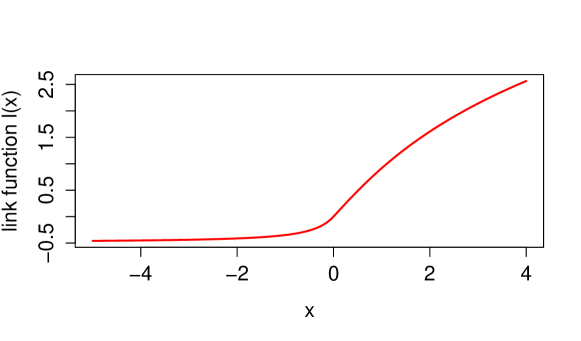
Figure 1: Link function for the shape of GEVD

To show that our choice of link function for GEVD, fulfills conditions (ii) and (iii), first we calculate its derivative $\dot{\ell}=\dot{f}/f$ and obtain $\dot{\ell}=(x+1)/(x^{2}/2+x+1)$ for $x>0$ and $\dot{\ell}=2a_{1}(a_{2}-x)^{-1}(\log(a_{2}-x))^{-3}$ for $x<0$. Hence, for large $x$, $\dot{\ell}$ behaves like $2/x$, while for $x<0$, it essentially behaves like $-x^{-1}(\log(-x))^{-3}$.

As mentioned, the term $\Gamma(2x)$ dominates all entries of all terms of $\mathcal{I}^{\scriptscriptstyle\mathcal{Q}}_{\sigma,\xi}$ in (3.3). Using the Stirling approximation, i.e., $\Gamma(x)\approx\sqrt{2\pi}\,\exp(x(\log(x)-1/2))$, due to the double application of the logarithm in the link function we get that $\Gamma(2\ell_{\xi}(\theta_{\xi}))$ is approximately $\beta_{\xi}\log(x_{\xi})$. By equivariance in $\mu$ and $\sigma$, therefore the integral of condition (ii) turns into: $B_{1}(\xi):=4\beta_{\xi}^{-1}\int\log(x)\,K(dx)<\infty$ for $\beta_{\xi}>0$ and, for $\beta_{\xi}<0$, to $B_{2}(\xi):=\beta_{\xi}^{-1}\int\,\log(x)\big{(}(\log(-\beta_{\xi})+\log(\log(x))\big{)}^{-6}\,K(dx)$. Finiteness of $B_{1}(\xi)$ and $B_{2}(\xi)$ follow from finiteness of $\mathop{\rm{{}E{}}}\nolimits(\min\{1,(\log x)^{k}\})$ for $x\sim\textrm{GEVD}(0,1,\xi)$, $k\in\textbf{N}$. Reconsidering $B_{1}(\xi)$, $B_{2}(\xi)$ at $\xi+s$, for $\left|s\right|<h$, $h<1$ we see that $\sup_{\left|s\right|<h}B_{i}(\xi+s)<\infty$ for $i=1,2$, hence, condition (iii) is a consequence of dominated convergence and continuity of Fisher information $I_{\xi\xi}$ in $\xi$.

References

- (1)
- Andrews et al. (2009) Andrews, B., Calder, M., and Davis, R.A. (2009): Maximum Likelihood Estimation for -Stable Autoregressive Processes. Annals of Statistics 37: 1946–1982.
- Bickel et al. (1993) Bickel, P.J., Klaassen, C.A.J., Ritov, Y., and Wellner, J. A. (1993): Efficient and adaptive inference in semiparametric models. Springer. New York.
- Cox (1981) Cox, D.R. (1981): Statistical Analysis of Time Series: Some Recent Developments. Scand. J. Statist. 8: 93–115.
- Dahen and Georges (2010) Dahen, H., and Georges, D. (2010): Scaling models for the severity and frequency of external operational loss data. Journal of Banking & Finance 34(7): 1484–1496.
- DuMouchel (1973) DuMouchel, W.H. (1973): On the asymptotic normality of the maximum likelihood estimate when sampling from a stable distribution. Annals of Statistics 1: 948- 957.
- Embrechts et al. (1997) Embrechts, P., Klüppelberg, C., and Mikosch, T. (1997): Modelling extremal events for insurance and finance. Springer. New York.
- Fahrmeir (1990) Fahrmeir, L. (1990): Maximum likelihood estimation in misspecified generalized linear models. Statistics 21(4): 487–502.
- Fahrmeir and Kaufmann (1985) Fahrmeir, L., and Kaufmann, H. (1985): Consistency and asymptotic normality of the maximum likelihood estimator in generalized linear models. The Annals of Statistics 13(1) 342–368.
- Fahrmeir and Tutz (2001) Fahrmeir, L. and Tutz, G. (2001): Multivariate Statistical Modelling Based on Generalized Linear Models. 2nd Edn. Springer. New York.
- Gouriéroux et al. (1984) Gouriéroux, C., Monfort, A., and Trognon, A. (1984): Pseudo maximum likelihood methods: Theory. Econometrica 52(3): 681–700.
- Haberman (1974) Haberman, S.J. (1974): Log-linear models for frequency tables with ordered classifications. Biometrics 30(4): 589–600.
- Haberman (1977) Haberman, S.J. (1977): Maximum likelihood estimates in exponential response models. The Annals of Statistics 5(5): 815–841.
- Hájek (1972) Hájek, J. (1972): Local asymptotic minimax and admissibility in estimation. In Proceedings of the sixth Berkeley symposium on mathematical statistics and probability. Vol. 1, pp. 175–194.
- Hallin et al. (2011) Hallin, M., Swan, Y., Verdebout, T., and Veredas, D. (2011): Rank-based testing in linear models with stable errors. Journal of Nonparametric Statistics 23: 305- 320.
- Huber (1981) Huber, P. (1981): Robust Statistics. Wiley. New York.
- Le Cam (1986) Le Cam, L. (1986): Asymptotic Methods in Statistical Decision Theory. Springer. New York.
- Le Cam (1970) Le Cam, L. (1970): On the assumptions used to prove asymptotic normality of maximum likelihood estimates. The Annals of Mathematical Statistics 41(3): 802–828.
- Le Cam and Young (2000) Le Cam, L., and Yang, G.L. (2000): Asymptotics in Statistics. Some Basic Concepts. (2nd ed.) Springer. New York.
- McCullagh and Nelder (1989) McCullagh, P., and Nelder, J.A. (1989): Generalized linear models. Chapman Hall. London.
- Nelder and Pregibon (1987) Nelder, J.A., and Pregibon, D. (1987): An Extended Quasi-Likelihood Function. Biometrika 74(2): 221–232.
- Nelder and Wedderburn (1972) Nelder, J.A., and Wedderburn, R.W.M. (1972): Generalized linear models. Journal of the Royal Statistical Society. Series A, 370–384.
- Rieder (1994) Rieder, H. (1994): Robust Asymptotic Statistics. Springer. New York.
- Rieder and Ruckdeschel (2001) Rieder, H., and Ruckdeschel, P. (2001): Short proofs on -Differentiability. Statistics & Decisions, 19: 419–425.
- Rudin (1986) Rudin, W. (1986): Real and complex analysis. 3rd Edn. McGraw-Hill Inc. New York.
- Schlather (1994) Schlather, M. (1994): Glattheit von Generalisierten Linearen Modellen und statistische Folgerungen. Diplomarbeit Universität Bayreuth.
- van der Vaart (1998) van der Vaart, A. (1998): Asymptotic Statistics. Cambridge University Press. Cambridge.
- Witting (1985) Witting, H. (1985): Mathematische Statistik. Parametrische Verfahren bei festem Stichprobenumfang. Teubner. Stuttgart.