Tree-based iterated local search for Markov random fields with applications in image analysis

Abstract

The maximum a posteriori (MAP) assignment for general structure Markov random fields (MRFs) is computationally intractable. In this paper, we exploit tree-based methods to efficiently address this problem. Our novel method, named Tree-based Iterated Local Search (T-ILS) takes advantage of the tractability of tree-structures embedded within MRFs to derive strong local search in an ILS framework. The method efficiently explores exponentially large neighborhood and does so with limited memory without any requirement on the cost functions. We evaluate the T-ILS in a simulation of Ising model and two real-world problems in computer vision: stereo matching, image denoising. Experimental results demonstrate that our methods are competitive against state-of-the-art rivals with a significant computational gain.

1 Introduction

Markov random fields (MRFs) [2, 13, 33] are popular probabilistic graphical representation for encoding the object’s state space using sites and the correlation between local objects using edges. For example, a grid is a powerful image representation for pixels, where each site represents a pixel state (e.g., intensity or label) and an edge represents local relations between neighboring pixels (e.g., smoothness). In other words, we can encode prior knowledge about the nature of interaction between objects in a MRF. Once the model has been built, we can perform inference in a principled manner.

One of the most important MRF inference problems in many applications is finding maximum a posteriori (MAP) assignment. The goal is to search for the the most probable state configuration of all objects, or equivalently, the lowest energy of the model. The problem is known to be NP-complete [7]. Given a MRF of $N$ objects each of which has $S$ states, a brute-force search must explore $S^{N}$ state configurations. In image denoising, for example, $N$ is the number of pixels, which can range from $10^{4}-10^{7}$, and $S$ is the number of pixel intensity levels, which are in the order of $2^{8}-2^{32}$. This calls for heuristic methods which can find reasonable solutions in practical time.

There have been a great number of attempts to solve this problem. An early approach was based on simulated annealing (SA), where the convergence is also guaranteed for log-time cooling schedule [13]. The main drawback of this approach is its low speed – it takes long time to achieve reasonably good solutions. Another early attempt involves local greedy search, and the iterated conditional mode (ICM) [3] is probably the most well-known method. In probabilistic terms, it iteratively seeks for the mode of the local distribution of states of an object conditioned on the states of nearby objects. Translated in combinatorial terms, it greedily searches for the local valley - here the neighborhood size is limited to $S$ - the number of possible states per object. Not surprisingly, this method is prone to getting stuck at poor local minima.

A more successful approach is belief-propagation (BP) [43], which exploits the problem structure better than the ICM. The main idea is that we maintain a set of messages sending simultaneously along all edges of the MRF network. A message carries the information of the state of the sites it originates from, and as a result, any update of a particular site is informed by messages from all nearby sites. However, this method can only be guaranteed to work for a limited class of network structures – when the network reduces to a tree, where there are no loops in the network. Another drawback is that the memory requirement for BP is high - this is generally linear in the number of edges in the network. More recently, efficient algorithms with theoretical guarantees have been introduced based on the theory of graph cuts [7]. This class of algorithms, while being useful in certain computer vision problems, has limitation in the range of problems it can solve – the energy formulation must admits a certain metric form [7, 50]. In effect, these algorithms are not applicable to problems where energy functions are estimated from data and their functional forms are not known in priori.

Given this ground, it is desirable to have an approximate algorithm which is fast enough (better than ICM - for example), consumes little memory and does not have any specific requirements of network structures or energy functionals. A meta-heuristic solution has already been proposed in the combinatorial optimization literature - the Iterated Local Search (ILS) (e.g. see [36]). Typically, ILS encourages jumping between local minima, which can be found by local search methods such as ICM. This algorithm, however, does not exploit any model-specific information, and thus could be inefficient for the MAP assignment in MRFs. To this end, we propose a novel algorithm called Tree-based Iterated Local Search (T-ILS), which combines the strength of BP and ILS. This algorithm exploits the fact that BP works efficiently on tree structures, in which the time complexity is linear in the number of edges in the tree, and thus BP is an effective candidate for locating good local minima. The main difference from standard tree-based BP is that our trees are conditional trees which are built upon fixing states of neighbor leaves. When combined with ILS, we have a heuristic algorithm that is less likely to get stuck in poor local minima, and has better chance to reach high quality solution, or even global minima.

We evaluate our tree-based inference methods on three benchmark problems: Ising model, stereo correspondence and image denoising. We empirically demonstrate that T-ILS attains good performance, while requiring less training time and memory than the loopy BP, which is one the state-of-the-arts for these problems.

To summarize, our main contributions are the proposal and evaluation of fast and lightweight tree-based inference methods in MRFs. Our choice of trees on $N=W\times H$ images requires only $\mathcal{O}(2D)$ memory where $D=\max\{W,H\}$ and two passes over all sites in the MRFs per iteration. These are much more economical than $\mathcal{O}(4WH)$ memory and many passes needed by the traditional loopy BP.

This paper is organized as follows. Section 3 describes MRFs, the MAP assignment problem, and belief propagation for trees. In Section 4, the concept of conditional trees is defined, followed by two algorithms: the strong local search T-ICM and the global search T-ILS. Section 5 provides empirical support for the performance of the T-ICM and T-ILS. Finally, Section 6 concludes the paper.

2 Related work

The MAP assignment for Markov random fields (MRFs) as a combinatorial search problem has attracted a great amount of research in the past several decades, especially in the area of computer vision [35] and probabilistic artificial intelligence [43]. The problem is known to be NP-hard [47]. For example, in labeling of an image of size $W\times H$, the problem space is $S^{WH}$ large, where $S$ is the number of possible labels per pixel.

Techniques for solving the MAP assignment can be broadly classified into stochastic and deterministic classes. In early days, the first stochastic algorithms were based on simulated annealing (SA) [22]. The first application of SA to Markov random fields (MRFs) with provable convergence was perhaps the work of [13]. The main drawback of this method is slow convergence toward good solutions [50]. Nature-inspired algorithms were also popular, especially the family of genetic algorithms [8, 20, 21, 38, 54]. Some attempts using ant colony optimization and tabu-search have also been made [42, 65].

Deterministic algorithms started in parallel with iterated conditional model (ICM) [3]. It is a simple greedy search strategy that updates one label at a time. Thus it is very slow and sensitive to bad initialization. A more successful approach is based on Pearl’s loopy belief propagation (BP) [43]. Due to its nature of using local information (called “messages”) to update “belief” about the optimal solution, loopy BP is also called a message passing algorithm. Although loopy BP is neither guaranteed to converge at all nor to reach global optima, empirical evidences so far have indicated that it is very competitive against state-of-the-arts in a variety of image analysis problems [12, 50]. Research on improving loopy BP is currently a very active topic in a range of disciplines, from artificial intelligence, statistical physics, computer visions to social network analysis [11, 12, 15, 18, 27, 28, 40, 66, 56]. The most recent development centers around convex analysis [17, 30, 44, 57, 60]. In particular, the MAP is converted into linear programming with relaxed constraints from which a mixture of convex optimization and message passing can be used. Loopy BP also plays role in improving evolutionary algorithms under probabilistic graphical model representation [32].

Another powerful class of algorithms in computer vision is graph cuts [7, 50]. They are, nevertheless, designed with specific cost functions in mind (i.e. metric and semi-metric) [26], and therefore inapplicable for generic cost functions such as those resulting from learning. Again, research in graph cuts is an active area in computer vision [4, 6, 23, 24, 29, 34]. Interestingly, it has been recently proved that graph cuts are in fact loop BP [51].

It is fair to say that the deterministic approach has become dominant due to their performance and theoretical guarantee for certain classes of problems [19]. However, the problem is still unsolved for general settings, thus motivates this paper. Our approach has both the deterministic and heuristic nature. It relies on the concept of strong local search using the deterministic method of BP, which is efficient in trees. The local search is strong because it covers a significant number of sites, rather than just one, which is often found in other local search methods such as ICM [3]. The neighborhood size in our method is very large [1]. For typical image labeling problems, the size is $S^{0.5WH}$ for an image of height $H$ and width $W$ and label size of $S$. Standard local search like ICM only explores the neighborhood of size $S$ at a time. Once a strong local minimum is found, a stochastic procedure based on iterated local search [36] is applied to escape from it and explores a better local minimum.

The idea of exploiting the trees in MRF in image analysis is not entirely new. In early days, a spanning tree is used to approximate the entire MRF [9, 16]. This method is efficient but the approximation quality may hurt because the number of edges in tree is far less than that in the original MRF. Another way is to built a hierarchical MRF with multiple resolutions [61], but this is less applicable for flat image labeling problems. Our method differs from these efforts in that we use trees embedded in the original graph rather than building an approximate tree. Second, our trees are conditional – trees are defined on the values of its leaves. Third, trees are selected as we go during the search process.

More recently, trees are used in variants of loop BP to specify the orders which messages are scheduled [57, 48]. Our method can also viewed along this line by differs in the way trees are built and messages are updated. In particular, our trees are conditional on neighbor labeling, which is equivalent to collapsing an associated message to a single value.

Iterated Local Search (ILS), also known as basin hopping [58], has been used in related applications such as image registration [10], and structure learning in probabilistic graphical models [5]. The success of ILS depends critically on the local search and the perturbation (basin hopping) strategy [37]. In [58], for example, a powerful local search based on conjugate gradients is essential to reach global solution for the Lennard-Jones clusters problem. Our work builds strong local search using tree-based BP on the discrete spaces rather than continuous ones.

3 Markov random fields for image labeling

In this section we introduce Markov random fields (MRFs) and the MAP assignment problem with application to image labeling. A MRF is a probabilistic way to express the uncertainty in the discrete system of many interacting variables each of which is characterized by a set of possible states [43]. In what follows, we briefly describe the MRF and its MAP assignment problem and focus on the minimization of model energy.

Formally, a MRF specifies a random field $\mathbf{x}=\{x_{i}\}_{i=1}^{N}$ over a graph $\mathcal{G}=(\mathcal{V},\mathcal{E})$, where $\mathcal{V}$ is the collection of $N$ sites $\{i\}$, $\mathcal{E}$ is the collection of edges $\{(i,j)\}$ between sites, and $x_{i}\in L$ represents states at site $i$. The entire system is random because the uncertainty in specifying the exact state of each site. One of the main objectives is to compute the most probable specification, also known as MAP assignment, which is the main focus of the paper.

3.1 Image labeling as energy minimization and MAP assignment

In image labeling problem, an image $\mathbf{y}$ is a collection of pixels arranged in a particular geometrical way, as defined by the graph $\mathcal{G}$. Typically, we assume a grid structure over pixels, where every inner pixel has exactly four nearby pixels. A labeling $\mathbf{x}$ is the assignment of each pixel $y_{i}$ a corresponding label $x_{i}$ for all $i=1,2,...,N$.

A full specification of an MRF over the labeling $\mathbf{x}$ given the image $\mathbf{y}$ can be characterized by its energy. Assuming pairwise interaction between connected sites, the energy is the sum of local energies as follows:

$$E(\mathbf{x},\mathbf{y}) = \sum_{i\in\mathcal{V}}E_{i}(x_{i},\mathbf{y})+\sum_{(i,j)\in\mathcal{E}}E_{ij}(x_{i},x_{j})$$ (1)

The singleton energy $E_{i}(x_{i},\mathbf{y})$ encodes the disassociation between the label $x_{i}$ and the features of image $\mathbf{y}$ at site $i$. In image denoising, for example, where $y_{i}$ is the corrupted pixel and $x_{i}$ is the true pixel we may use $E_{i}(x_{i},\mathbf{y})=\left|x_{i}-y_{i}\right|$ as the cost due to corruption. The pairwise energy $E_{ij}(x_{i},x_{j})$ often captures the smoothness nature of image, that is, two nearby pixels tend to be similar. For example, $E_{ij}(x_{i},x_{j})=\lambda\left|x_{i}-x_{j}\right|$ is a cost of difference between two labels, where $\lambda>0$ is a problem-specific parameter.

In image labeling, the task is to find the optimal $\mathbf{x}^{map}$ that minimizes the energy $E(\mathbf{x},\mathbf{y})$, which now plays the role of the cost function:

$$\mathbf{x}^{map} = \arg\min_{\mathbf{x}}E(\mathbf{x},\mathbf{y})$$ (2)

For example, in image denoising, this translates to finding a map of intensity that admits both the low cost of corruption and high smoothness.

The formal justification for the energy minimization in MRF can be found through the probability of the labeling defined as

$$P(\mathbf{x}\mid\mathbf{y})=\frac{1}{Z(\mathbf{y})}e^{-E(\mathbf{x},\mathbf{y})}$$ (3)

where $Z(\mathbf{y})$ is the normalization term. Thus minimizing the energy is equivalent to finding the most probable labeling $\mathbf{x}^{map}$. As $P(\mathbf{x}\mid\mathbf{y})$ is often called the posterior distribution in computer vision, the energy minimization problem is also referred to as maximum a posteriori (MAP) assignment.

3.2 Local search: Iterated conditional mode

Iterated conditional mode (ICM) [3] is a simple local search algorithm. It iteratively finds the local optimal labeling for each site $i$ as follows

$$x_{i}^{*} =\arg\min_{x_{i}} \left\{E_{i}(x_{i},\mathbf{y})+\sum_{j\in\mathcal{N}(i)}E_{ij}(x_{i},x_{j})\right\}$$ (4)

where $\mathcal{N}(i)$ is the set of sites connected to the site $i$, often referred to as Markov blanket. The Markov blanket shields a site from the long-range interactions with remote sites, due to a special property of MRF known as Markov property, which states that probability of a label assignment at site $i$ given all other assignments depends only on the nearby assignments [14, 33]. The probabilistic interpretation of Eq. (4) is

$$x_{i}^{*}=\arg\max_{x_{i}}P\left(x_{i}\mid\{x_{j}\}_{j\in\mathcal{N}(i)},\mathbf{y}\right)$$

The local update in Eq. (4) is repeated for all sites until no more improvement can be made. This procedure is guaranteed to find a local minimum energy in a finite number of steps. However, the solutions found by the ICM are sensitive to initialization and often unsatisfactory for image labeling [50].

3.3 Exact global search on trees: Belief-propagation

Figure 1: Belief propagation on trees: the two-pass procedure.

Belief-propagation (BP) was first proposed as an inference method on MRF with tree-like structures in the field of artificial intelligence [43]. BP operates by sending messages between connecting sites. For this reason, it is also called message passing algorithm. It is efficient because instead of dealing with all the sites simultaneously, we need to compute messages passing between two local sites. At each site, local information modifies the incoming messages before sending out to neighbor sites.

General BP.

The general rule is that the message sent from site $j$ to site $i$ in the tree is computed as follows

$$\mu_{j\rightarrow i}(x_{i}) = \min_{x_{j}}\left(E_{j}(x_{j},\mathbf{y})+E_{ij}(x_{i},x_{j})+\sum_{k\in\mathcal{N}(j),k\neq i}\mu_{k\rightarrow j}(x_{j})\right)$$ (5)

That is, the outgoing message is aggregated from all incoming messages, except for the one in the opposite direction. Messages can be initialized arbitrarily, and the procedure is guaranteed to stop after finite steps on trees [43]. The optimal labeling could be estimated as follows

$$x_{i}^{map}=\arg\min_{x_{i}}\left(E_{i}(x_{i},\mathbf{y})+\sum_{k\in\mathcal{N}(i)}\mu_{k\rightarrow i}(x_{i})\right)$$ (6)

It has been proved that the labeling obtained in this way is indeed globally optimal [43], i.e.,

$$\mathbf{x}^{map}=\arg\min_{\mathbf{x}}E(\mathbf{x},\mathbf{y})$$

2-pass BP.

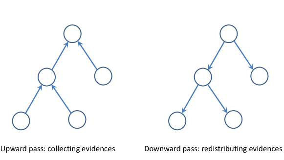
A more efficient variant of BP is the 2-pass procedure, as summarized in Fig. 1. First we pick one particular site as the root. Since the graph has no loops, there is a single path from a site to any other sites in the graph, and each site, except for the root, has exactly one parent. The procedure consists of two passes:

• Upward pass: Messages are first initiated at the leaves, and are set to $0$. Then all messages are sent upward and updated as messages converging at common parents along the paths from leaves to the root. The pass stops when all the messages reach the root.

• Downward pass: Messages are combined and re-distributed downward from the root back to the leaves. The messages are then terminated at the leaves.

The 2-pass BP procedure is a remarkable algorithm: it searches through the combinatorial space of $S^{N}$ using only $\mathcal{O}\left(2NS^{2}\right)$ operations and $\mathcal{O}\left(2NS\right)$ memory to store all the messages.

Remark.

We note in passing that this procedure may be known as min-sum, max-product, or simply BP. The term max-product comes from the fact that we can operate in the potential domain by taking the exponential of negative energies in Eqs. (5,6), and turn mins into maxes and sums into products.

3.4 Approximate global search on general graphs: Loopy belief-propagation

Standard MRFs in image analysis are usually not tree-structured. A common topology is a grid in which each site represents a pixel and has four neighbors. Thus the resulting graph has many cycles, rendering the standard 2-pass BP algorithm useless.

However, an approximation to exact BP has been suggested. Using the general BP described above, messages are sent across all edges without worrying about the order [43]. At each step, the messages are updated using Eq. (5). After some stopping criteria are met, we still use Eq. (6) to find the best labeling. This procedure is often called loopy BP due to the presence of loops in the graph. The heuristic has been shown to be useful in several applications [41] and this has triggered much research on improving it [11, 12, 25, 49, 45, 57, 55, 59, 64, 63].

The main drawback of loopy BP is lack of convergence guarantee for general problems. In our simulation of Ising models (Sec. 5.1), loop BP clearly fails in the cases where interaction energies dominate singleton energies, that is $\left|E_{ij}(x_{i},x_{j})\right|\gg\left|E_{i}(x_{i},\mathbf{y})\right|$ for all $i,j$ (see Fig. 4). Another drawback is that the memory will be very demanding for large images. For grid-image, the memory needed is $\mathcal{O}\left(4HWS\right)$ which in the order of gigabytes, and thus may not be suitable for devices with small footprint.

4 Iterated strong local search

In this section we present a method to exploit the efficiency of the BP on trees to build strong local search for the MAP assignment problem in Markov random fields. By ‘strong’, we mean the quality of the local solution found by the procedure is often much better than standard greedy local search. Although a typical MRF in computer vision is not a tree, we observe that it can be thought as a super-imposition of trees. Second, due to the Markov property of MRFs, described in Sec. 3.2, variables in a tree can be shielded from other variables through the Markov blanket of the tree. This gives rise to the concept of conditional trees, which we present subsequently.

4.1 Conditional trees

Figure 2: Examples of conditional trees on grid (connecting empty sites). Filled nodes are labeled sites. Arrows indicate absorbing direction, dashes represent unused interactions. Dotted lines in (c,d) are dummy edge (with zeros interacting energy) that connects separate sub-trees together to form a full tree.

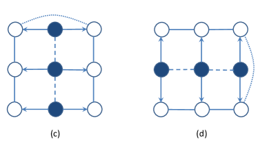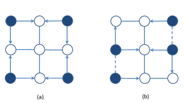
For concreteness, let us consider grid-structured MRFs. There are more than one way to extract a tree out of the grid, as shown in Fig 2. In particular, we fix some labeling to some sites, leaving the rest forming a tree. Consider a tree $\tau$ and let $\mathbf{x}_{\tau}=\{x_{i}\mid i\in\tau\}$, and $\mathbf{x}_{\neg\tau}=\{x_{i}\mid i\notin\tau\}$. Denote by $\mathcal{N}(\tau)$ the set of sites connecting to $\tau$ but do not belong to $\tau$. This is essentially the Markov blanket of the tree $\tau$. Thus the collection of sites $\left(\tau,\mathcal{N}(\tau)\right)$ and the partial labeling of the neighbor sites $\mathbf{x}_{\mathcal{N}(\tau),}$ forms a conditional tree. The energy of the conditional tree can be written as:

$$E_{\tau}\left(\mathbf{x}_{\tau},\mathbf{x}_{\mathcal{N}(\tau)},\mathbf{y}\right) = \sum_{i\in\tau}E_{i}^{*}(x_{i},\mathbf{y})+\sum_{i,j\in\tau}E_{ij}(x_{i},x_{j})$$ (7)

where

$$E_{i}^{*}(x_{i},\mathbf{y})=E_{i}(x_{i},\mathbf{y})+\sum_{(i,j)\in\mathcal{E},j\in\mathcal{N}(\tau)}E_{ij}(x_{i},x_{j})$$ (8)

In other words, the interacting energies at the tree border are absorbed into the singleton energy of the ordering sites. In Fig. 2 the absorbing direction is represented by an arrow.

The minimizer of this conditional tree energy can be found efficiently using the BP:

$$\hat{\mathbf{x}}_{\tau}=\arg\min_{\mathbf{x}_{\tau}}E_{\tau}\left(\mathbf{x}_{\tau},\mathbf{x}_{\mathcal{N}(\tau)},\mathbf{y}\right)$$ (9)

This is due to the fact that Eq. (7) now has the form of Eq. (1).

One may wonder how the minima of the energy of conditional trees $E_{\tau}\left(\mathbf{x}_{\tau},\mathbf{x}_{\mathcal{N}(\tau)},\mathbf{y}\right)$ relate to the minima of the entire systems $E\left(\mathbf{x},\mathbf{y}\right)$. We present here two theoretical results of this connection. First, the local minimum found by Eq. (9) is also a local minimum of $E\left(\mathbf{x},\mathbf{y}\right)$:

Proposition 1

Finding the mode $\hat{\mathbf{x}}_{\tau}$ as in Eq. (9) guarantees a local minimization of model energy over all possible tree labelings. That is

$$E(\hat{\mathbf{x}}_{\tau},\mathbf{x}_{\neg\tau},\mathbf{y})\leq E(\mathbf{x}_{\tau},\mathbf{x}_{\neg\tau},\mathbf{y})$$

for all $\mathbf{x}_{\tau}\neq\hat{\mathbf{x}}_{\tau}$.

Proof:

The proof is presented in Appendix A.2.

The second theoretical result is that the local minimum found by Eq. (9) is indeed the global minimum of the entire system if all other labels outside the tree happen to be part of the optimal labeling:

Proposition 2

If $\mathbf{x}_{\neg\tau}\in\mathbf{x}^{map}$ then $\hat{\mathbf{x}}{}_{\tau}\in\mathbf{x}^{map}$.

Proof:

We first observe that since $E(\mathbf{x}^{map},\mathbf{y})$ is the lowest energy then

$$E(\mathbf{x}^{map},\mathbf{y}) \leq E(\hat{\mathbf{x}}_{\tau},\mathbf{x}_{\neg\tau},\mathbf{y})$$ (10)

Now assume that $\hat{\mathbf{x}}_{\tau}\notin\mathbf{x}^{map}$, so there must exist $\mathbf{x}^{\prime}_{\tau}\in\mathbf{x}^{map}$ that $\hat{\mathbf{x}}_{\tau}\neq\mathbf{x}^{\prime}_{\tau}$ and $E(\mathbf{x}^{\prime}_{\tau},\mathbf{x}_{\neg\tau},\mathbf{y})>E(\hat{\mathbf{x}}_{\tau},\mathbf{x}_{\neg\tau},\mathbf{y})$, or equivalently $E(\mathbf{x}^{map},\mathbf{y})>E(\hat{\mathbf{x}}_{\tau},\mathbf{x}_{\neg\tau},\mathbf{y})$, which contradicts with Eq. (10) $\blacksquare$

The derivation in Eq. (7) from the probabilistic formulation is presented in Appendix. A.1.

4.2 Tree-based ICM (T-ICM): conditional trees for strong local search

As conditional trees can be efficient to estimate the optimal labeling, we propose a method in the spirit of the simple local search ICM [3] (Section 3.2). First of all, a set of conditional trees $\mathcal{T}$ is constructed. At each step, a tree $\tau\in\mathcal{T}$ is picked according to predefined rules. Using the 2-step procedure of BP, we find the optimal labeling for $\tau$ using Eq. (9). This method includes the ICM as a special case when the tree is reduced to a single site, so we call it the tree-based ICM (T-ICM) algorithm, which is presented in pseudo-code in Algorithm 1.

Function: T-ICM()

Input:

• Graph $\mathcal{G}=(\mathcal{V},\mathcal{E})$.

• Local cost/energy functions $E_{i}(x_{i},\mathbf{y})$ and $E_{ij}(x_{i},x_{j})$.

• A set of trees $\mathcal{T}$, and an update schedule.

• Maximum number of iterations $T$.

• Initial labeling $\mathbf{x}^{0}$.

Procedure:

   For $t=1,2,...,T$

      1. Pick a conditional tree $\tau$ from the tree set $\mathcal{T}$ according to the update schedule.

      2. Absorb neighboring energies according to Eq. (8).

      3. Run $2$-pass BP on the conditional tree (Section 3.3): $\mathbf{x}_{\tau}^{t}\leftarrow BP(\mathbf{x}_{\tau}^{t-1})$.

      4. Update the labeling of the tree: $\mathbf{x}_{\tau}^{t}\leftarrow\mathbf{x}{}_{\tau}^{t-1}$.

      5. Stop if $E_{\tau}\left(\mathbf{x}_{\tau}^{t},\mathbf{x}_{\mathcal{N}(\tau)}^{t},\mathbf{y}\right)$ no longer decreases for all trees $\tau\in\mathcal{T}$.

Output: A local optimal labeling.

Algorithm 1 Tree-based iterated conditional mode (T-ICM).

4.2.1 Specification of T-ICM

Tree set and update schedule.

For a given graph, there are exponentially many ways to build conditional trees, and thus defining the tree set is itself a nontrivial task. However, for grids used in image labeling with height $H$ and width $W$, we suggest two simple ways:

• The set of $H$ rows and $W$ columns. The neighborhood of size is $HS^{W}+WS^{H}$.

• The set of $2$ alternative rows and $2$ alternative columns (Figs. 2c,d). Since alternative rows (or columns) are separated, they can be connected by dummy edges to form a tree (e.g., see Figs. 2c,d). A dummy edge has the interacting energy of zero, thus does not affect search operations on individual components. The neighborhood size is $4S^{0.5HW}$.

These two sets lead to much more efficient T-ICM compared to the standard ICM which only covers the neighborhood of size $SHW$ using the same running time. Once the set has been defined, the update order for trees can be predefined (e.g., rows from-top-to-bottom then columns from-left-to-right), or random.

4.2.2 Properties of T-ICM

Due to Proposition 1, at each step of Algorithm 1, the total energy $E(\mathbf{x},\mathbf{y})$ will be either reduced or the algorithm will terminate. Since the model is finite and the energy reduction is discrete (hence non-vanishing), the algorithm is guaranteed to reach a local minimum after finite steps.

Although the T-ICM only finds local minima of the energy, we can expect the quality to be better than the original ICM because each tree covers many sites. For example, as shown in Figs. 2a,b, a tree in the grid can account for half of all the sites, which is overwhelmingly large compared to a single site used by the ICM. The number of configurations of the tree $\tau$, or equivalently the neighborhood size, is $S^{N_{\tau}}$, where $N_{\tau}$ is the number of sites on the tree $\tau$. The neighborhood size of the ICM, on the other hands, is just $S$.

For the commonly used $4$-neighbor grid MRF in image labeling, and the tree set of alternative rows and columns, the BP takes $\mathcal{O}(4HW)$ time to pass messages, each of which cost $3S^{2}$ time to compute. Thus, the time complexity per iteration of T-ICM is only $S$ times higher than that of ICM and about the same as that of loop BP (Sec. 3.4). However, the memory in our case is still $\mathcal{O}\left(2\times\max\{H,W\}\right)$, which is much smaller than the $\mathcal{O}(4HW)$ memory required by loopy BP. In addition, each step in T-ICM takes exactly 2 passes, while the number of iterations of loopy BP for the whole image, if the method does converge, is unknown and parameter dependent.

4.3 Tree-based ILS: global search

Function: T-ILS()

Input:

• Max jump step-size: $\rho_{max}\in(0,100)$.

• Max number of iterations $T_{outter}$; max number of iterations for the inner T-ICM $T_{inner}$.

• Max number of backtracks.

Procedure:

   Initialize some labelings: $\tilde{\mathbf{x}}^{0}$.

   Find the first local minimum: $\mathbf{x}^{1}\leftarrow\mbox{T-ICM}\left(\tilde{\mathbf{x}}^{0},T_{inner}\right)$.

   Initialize variables: $n=0$; $\beta=1$.

   For $t=1,2,...,T_{outter}$

      1. Jump to a new place: $\tilde{\mathbf{x}}^{t}\leftarrow\mathbf{x}^{t}$ by randomly resetting $\mathcal{U}\left(0,\rho_{max}\right)\%$ of labels.

      2. Find a local minimum: $\hat{\mathbf{x}}^{t+1}\leftarrow\mbox{T-ICM}\left(\tilde{\mathbf{x}}^{t},T_{inner}\right)$.

      3. Accept: $\mathbf{x}^{t+1}\leftarrow\hat{\mathbf{x}}^{t+1}$ with probability of

                  $a=\min\left\{1,\exp\left(-\beta\left\{E(\hat{\mathbf{x}}^{t+1},\mathbf{y})-E(\mathbf{x}^{t},\mathbf{y})\right\}\right)\right\}$

         otherwise backtrack: $\mathbf{x}^{t+1}\leftarrow\mathbf{x}^{t}$ .

      4. Adjust the temperature:

                  $n\leftarrow n+1$ if $\mathbf{x}^{t+1}=\hat{\mathbf{x}}^{t+1}$;

                  $r\leftarrow 0.9n/t+0.1\mathbb{I}\left[\mathbf{x}^{t+1}=\hat{\mathbf{x}}^{t+1}\right]$ ;

                  if $r<0.45$ then $\beta\leftarrow 0.8\beta$ else if $r>0.55$ then $\beta\leftarrow\beta/0.8$.

      5. Stop if number of backtracks has been reach.

Output: A near global optimal labeling.

Algorithm 2 Tree-based iterated local search (T-ILS).

As T-ICM is still a local search procedure, inherent drawbacks still remain: (i) it is sensitive to initialization, and (ii) it can get stuck in suboptimal solutions. To escape from the local minima, global search strategies must be employed. We can consider the entire T-ICM as a single super-move in an exponentially large neighborhood.

Figure 3: Search behavior of T-ICM and T-ILS. The use of T-ICM creates a smoother energy landscape for T-ILS (the surrogate dotted curve). ICM gets stuck on the first local minimum it finds, but T-ICM could find a much better solution by operating on an exponentially large neighborhood.

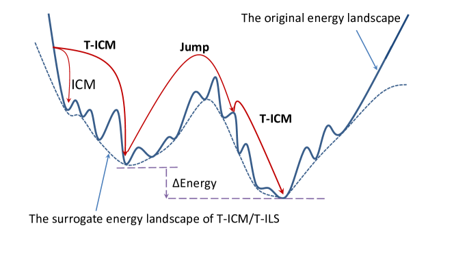
Since it is not our intention to create a totally new escaping heuristic, we draw from the rich pool of metaheuristics in the literature and adapt to the domain of image labeling. In particular, we choose an effective heuristic, commonly known as iterated local search (ILS) [36] for escaping from the local minima. ILS advocates jumps from one local minimum to another with the hope that we can eventually find better local minima after multiple tries. If a jump fails to lead to a better solution, it can still be accepted according to an acceptance scheme, following the spirit of simulated annealing (SL). However, we do not decrease the temperature as in the SL, but rather, the temperature is adjusted so that on average the acceptance probability is roughly $0.5$. The process is repeated until the stopping criteria are met. We term the resulting metaheuristic the Tree-based Iterated Local Search (T-ILS) whose pseudo-code is presented in Algorithm 2, and behavior is illustrated in Fig. 3. In what follows we specify the algorithm in more details.

4.3.1 Specification of T-ILS

Jump.

The jump step-size has to be large enough to successfully escape from the basin that traps the local search. In this study, we design a simple jump by randomly changing labels of $\rho\%$ of sites. The step-size $\rho$ is drawn randomly in the range $(0,\rho_{max})$, i.e., $\rho\sim\mathcal{U}\left(0,\rho_{max}\right)$, where $\rho_{max}$ is an user-specified parameter.

Acceptance.

After a jump, the local search is invoked, followed by an acceptance decision to accept or reject the jump. Convergence guaranteed acceptance criteria such as those used in simulated annealing can be used, but it is likely to be slow. We consider the following acceptance probability:

$$a=\min\left\{1,\exp(-\beta\Delta E)\right\}$$

where $\Delta E=E(\hat{\mathbf{x}}^{t+1},\mathbf{y})-E(\mathbf{x}^{t},\mathbf{y})$ is the change in energy between two consecutive minima, and $\beta>0$ is the adjustable “inverse temperature”. Large $\beta$ lowers the acceptance rate but small $\beta$ increases the rate. This fact will be used to adjust the acceptance rate, as detailed below.

Adjusting inverse temperature.

We wish to maintain an average acceptance probability of $0.5$, following the success of [58]. However, unlike the work in [58], we do not change the step-size, but rather adjusting the inverse temperature. The estimation of acceptance rate is $r\leftarrow r/t$, where $n$ is the total number of accepted jumps up to step $t$. To introduce short-term effect, we use the last event:

$$r\leftarrow 0.9r+0.1\mathbb{I}\left[\mathbf{x}^{t+1}=\hat{\mathbf{x}}^{t+1}\right]$$

If the acceptance rate is within the range $[0.45,0.55]$ we do nothing. A lower rate will lead to decrease of the inverse temperature: $\beta\leftarrow 0.8\beta$, and a higher rate will lead to increase: $\beta\leftarrow\beta/0.8$.

4.3.2 Properties of T-ILS

Fig. 3 illustrates the behavior of the T-ILS. Through the T-ICM component, the energy landscape is smoothed out, helping the T-ICM to locate good local minima. When the jump is not large, the search trajectory can be tracked to avoid self-crossing walks. If the jump is far enough (with large $\rho_{max}$), the resulting algorithm will behave like the well-known multistart procedures.

When the inverse temperature $\beta$ is set to $0$, the acceptance become deterministic, that is, we only accept the jump if it improves the current solution. In other words, the T-ILS becomes a greedy algorithm. Alternatively, when $\beta$ is set to a very large number and no adjustment is made, we would accept all the jumps, allowing memoryless foraging behavior.

5 Experiments

In this section, we evaluate our proposed algorithms on a simulated Ising model and two standard vision labeling problems: stereo correspondence and image denoising. In all settings, we employ MRFs with grid-structure (e.g. each inner pixel is connected to exactly 4 nearby pixels). Trees are composed of rows and columns as specified in Sec. 4.2.1. Unless specified otherwise, the initial labeling is randomly assigned. Max step-size is $\rho_{max}=10\%$ (Sec. 4.3.1). For T-ILS, the inner loop has $T_{inner}=1$, i.e., the full local minima may not be reached by the T-ICM, as does not seem to hurt the final performance.

5.1 Simulated Ising model

In this subsection, we validate the robustness of our proposed algorithms on Ising models, which have wide applications in magnetism, lattice gases, and neuroscience [39]. Within the MRF literature, Ising lattice is often used as a benchmark to test inference algorithms (e.g., see [57]). Following [57], we simulate a 500$\times$500 grid Ising model where labels are binary spin orientations (up or down): $x_{i}\in\pm 1$, and local energy functions are: $E_{i}(x_{i})=\theta_{i}x_{i}$; $E_{ij}(x_{i},x_{j})=\theta_{ij}x_{i}x_{j}$. The parameter $\theta_{i}$ specifies the influence of external field on the spin orientation and $\theta_{ij}$ specifies the interaction strength and direction (impulsive or repulsive) between sites. For this experiment, the parameters $\left\{\theta_{i},\theta_{ij}\right\}$ are set as follows

$$\theta_{i},\theta_{ij} \sim \mathcal{U}(-1,1)$$

where $\mathcal{U}(-1,1)$ denotes the uniform distribution in the range $(-1,1)$, and $\lambda>0$ specifies the interaction strength. When $\lambda$ is small, the interaction is weak, and thus the external field has more effect on the spin arrangement. However, when $\lambda$ is large, the spin arrangement depends more on the interacting nature. A stable arrangement in nature would be of the minimum energy.

The result of minimizing energy is shown in Fig. 4. When the interaction is weak (e.g. $\lambda=0.5$), the loopy BP performs well, but when the interaction is strong (e.g. $\lambda=1.0$), the T-ILS has a clear advantage. Thus T-ILS is more robust since it is less sensitive to $\lambda$.

Figure 4: Performance of T-ILS and loopy BP algorithm in minimizing Ising energy with $\lambda=0.5$ (left) and $\lambda=1.0$ (right).

5.2 Stereo correspondence

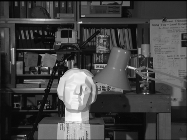
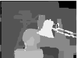
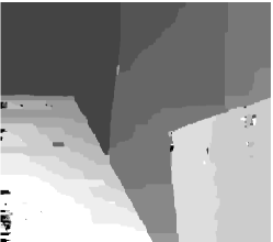
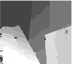
The problem in stereo correspondence is to estimate the depth of the field (DoF) given two or more 2D images of the same scene taken from two or more cameras arranged horizontally. This is used in 3D reconstruction of a scene using standard 2D cameras. The problem is often translated into estimating disparity between images – how much two images differ and this reflects the depth at any pixel locations. For simplicity, we only investigate the two-cameras setting. In the MRF-based stereo framework, a configuration of $\mathbf{x}\in\mathbb{N}^{W\times H}$ realizes the disparity map, which in this case is represented by a grid network. The disparity set (or the label set) is often predefined. For example, in the two standard datasets used in this experiment, the Tsukuba has $16$ labels (Fig. 5), and the Venus has $20$ (Fig. 6).

Figure 5: Stereo results on the Tsukuba dataset. (Top-left): left image, (top-middle): right image, (top-right): groundtruth; (bottom-left): scan-line, (bottom-middle): loop BP, and (bottom-right): T-ILS (initialized from scan-line).

Figure 6: Stereo results on the Venus dataset. (Top-left): left image, (top-middle): right image, (top-right): groundtruth; (bottom-left): scan-line, (bottom-middle): loop BP, and (bottom-right): T-ILS (initialized from scan-line).

The singleton energy $E_{i}(x_{i},\mathbf{y})$ at each pixel location usually measures the dissimilarity of pixel intensity between the left/right images, and the interaction energy $E_{ij}(x_{i},x_{j})$ ensures the smoothness of the disparity map. In this set of experiments, we use the simple linear Potts cost model as often used in testing stereo correspondence algorithms [46]. Let $\mathbf{y}=(I^{l},I^{r})$ where $I^{l}$ and $I^{r}$ are intensities of the left and right images respectively, and $i=(i_{X},i_{Y})$ where $i_{X}$ and $i_{Y}$ are horizontal and vertical coordinates of the pixel $i$. The local energies are defined as [46]:

$$E_{i}(x_{i},\mathbf{y}) = \Delta I(i,x_{i})$$

$$E_{ij}(x_{i},x_{j}) = \lambda\times\mathbb{I}[x_{i}\neq x_{j}]$$

where $\mathbb{I}[\cdot]$ is the indicator function, $\lambda>0$ is the smoothness parameter, and$\Delta I(i,x_{i})=\left|I^{l}(i_{X},i_{Y})-I^{r}(i_{X}-x_{i},i_{Y})\right|$ is the difference in pixel intensity in two images when pixel positions are $x_{i}$ pixels apart in the horizontal dimension. Due to the optical properties of two nearby cameras, a small $x_{i}$ would result in large $\Delta I(i,x_{i})$ if the true DoF is small. Thus by minimizing the singleton energy with respect to $x_{i}$, a small DoF would leads to stronger reduction of $x_{i}$ than a large DoF. For this set of experiments, we choose $\lambda=20$ following [46]. Our implementation is based on the software framework of [50].

There is a wide range of techniques available for stereo estimation, and loopy BP is one of the winning methods [46][50]. Fast methods like scan-line (SL) optimization are still widely used for real-time implementation. The scan-line is equivalent to taking independent 1D rows of the MRF and running the chain BP. Since the SL does not admit the original 2D structure, we need to adapt the singleton energy as: $\bar{E}_{i}(x_{i},\mathbf{y})=\nu E_{i}(x_{i},y)$ where $\nu\in[0,1]$ to account for the lack of inter-row interactions.

Method	Tsukuba	Venus
SL($\nu=1.0$)	814,121	1,362,067
SL($\nu=0.4$)	658,946	1,198,324
Random$\rightarrow$T-ICM($T=1)$	739,370	1,048,587
SL($\nu=0.4$)$\rightarrow$T-ICM($T=1)$	427,860	669,973
Loopy BP($T=1,000$)	413,269	640,385
SL($\nu=0.4$)$\rightarrow$T-ILS($T_{outter}=1,000$)	403,129	635,305

Table 1: Stereo energy found by algorithms. SL=Scan-line.

Tsukuba (Fig. 5)	Venus (Fig. 6)

Figure 7: Stereo energy minimization by Loopy BP (dashed line) and T-ILS (line) on Tsukuba (left) and Venus (right) images.

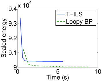
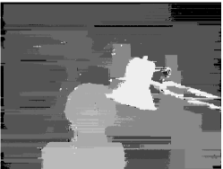
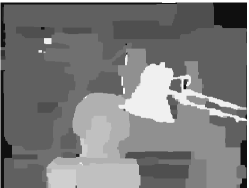
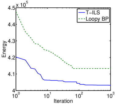
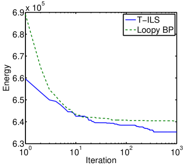
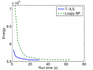
Table 1 shows the effect of changing from $\nu=1.0$ to $\nu=0.4$ in term of reducing 2D energy and error. The result, however, has the inherent horizontal ‘streaking’ effect since no 2D constraints are ensured (Figs. 5,6, bottom-left). The randomly initialized T-ICM with one iteration ($T=1$ in Algorithm 1) performs comparably with the best of SL ($\nu=0.4$). The performance of T-ICM improves significantly by initializing from the result of SL. T-ILS initialized from SL finds better energy than the loopy BP given the same number of iterations, as shown in Fig. 7.

5.3 Image denoising

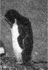
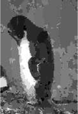
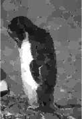
In image denoising, we are given an image corrupted by noise, and the task is to reconstruct the original image. For this set of experiments we use the $122\times 179$ noisy gray Penguin image (Fig. 8). The labels of the MRF correspond to $S=256$ intensity levels ($8$ bits depth). Similar to the stereo correspondence problem, we use a simple truncated Potts model for the energy as follows

$$E_{i}(x_{i},\mathbf{y}) = \min\left\{|x_{i}-y_{i}|,\tau\right\}$$

$$E_{ij}(x_{i},x_{j}) = \lambda\times\delta[x_{i}\neq x_{j}]$$

where $\tau=100$ prevents the effect of extreme noise, and $\lambda=25$ is smoothness parameter, following [50]. In addition, the optimized loopy BP for Potts models from [12] is used. Figs 8(b,c) demonstrates that T-ILS runs faster than the optimize loopy BP, yielding lower energy and smoother restoration.

(a)	(b)	(c)	(d)

Figure 8: Penguin images: (a) noisy, (b) restored with T-ILS, (b) restored with loopy BP; (d) running time. Algorithms stop after $5$ unsuccessful iterations.

6 Discussion

We have proposed a fast method for inference in Markov random fields by exploiting tree structures embedded in the network. We proposed a strong local search operator (T-ICM) based on Belief-Propagation and a global stochastic search operator T-ILS based on the iterated local search framework. We have shown in both simulation and two real-world image analysis tasks (stereo correspondence and image denoising) that the T-ILS is competitive against state-of-the-art algorithms. We have demonstrated that by exploiting the structure of the domains, we can derive strong local search operators which can be exploited in a metaheuristic strategy such as ILS.

6.1 Future work

The line of current work could be extended in several directions. First, we could adapt the T-ILS for certain cost functions. Currently, the T-ILS is designed as a generic optimization method, making no assumptions about the the nature of optimal solution. In contrast, label maps in vision are often smooth almost everywhere except for sharp boundaries. Second, the MRFs may offer a more informative way to perform the jump steps, e.g., by relaxing the messages in the local edges or by keeping track of the hopping trajectories. Third, we have limited the T-ILS to uniform distribution of step-sizes, but it needs not be the case. One useful heuristic is Lévy flights [52, 62] in which the step-size $\rho$ is drawn from the power-law distribution: $\rho^{-\alpha}$ for $\alpha>0$. This distribution allows the step-size to usually stay within a certain narrow range but also allows occasional big jump (which might behave like a total restart). Alternatively, we can use Beta distribution due to its richness in distribution shape and the boundedness of $\rho$. Fourth, since a MRF typically contain many separated conditional trees, it could be interesting to explore the parallel jump strategies.

As our development is based on the recognition that we can exploit conditional trees in MRFs to obtain fast strong local search. The metaheuristics thus need not be limited to ILS. In fact, conditional trees open up a new direction of research in the MAP assignment by investigating the use of other metaheuristics. For example, we can use genetic algorithms in conjunction with the conditional trees as follows. Each individual in the GA population can be represented by a string of $N$ characters, each of which has one of $S$ values in the label alphabet. For each individual, we run the 2-pass BP to obtain a strong local solution. Then the crossover operator can be applied character-wise on a selected subset to generate a new population.

Finally, although we have limited ourselves to applications in image analysis, the proposed algorithm is generic to any problems where MRFs are applicable.

Appendix A Appendix

A.1 Distribution over conditional trees

We provide the derivation of Eq. (7) from the probabilistic argument. Recall that $\mathcal{N}(\tau)$ is the Markov blanket of the tree $\tau$, that is, the set of sites connecting to $\tau$. Due to the Markov property

$$P\left(\mathbf{x}_{\tau}\mid\mathbf{x}_{\mathcal{N}(\tau)},\mathbf{y}\right)=P\left(\mathbf{x}_{\tau}\mid\mathbf{x}_{\neg\tau},\mathbf{y}\right)$$

In other words, we need only to worry about the interaction within the tree, and between the tree sites with its Markov blanket:

$$P\left(\mathbf{x}_{\tau}\mid\mathbf{x}_{\mathcal{N}(\tau)},\mathbf{y}\right)\propto\exp\left\{-E_{\tau}\left(\mathbf{x}_{\tau},\mathbf{x}_{\mathcal{N}(\tau)},\mathbf{y}\right)\right\}$$

where

$$E_{\tau}\left(\mathbf{x}_{\tau},\mathbf{x}_{\mathcal{N}(\tau)},\mathbf{y}\right) = \sum_{i\in\tau}E_{i}(x_{i},\mathbf{y})+\sum_{(i,j)\in\mathcal{E}\mid i,j\in\tau}E_{ij}(x_{i},x_{j})+\sum_{(i,j)\in\mathcal{E}\mid i\in\tau,j\in\mathcal{N}(\tau)}E_{ij}(x_{i},x_{j})$$ (11)

Eq. (7) can be derived from the energy above by letting:

$$E_{i}^{*}(x_{i},\mathbf{y})=E_{i}(x_{i},\mathbf{y})+\sum_{(i,j)\in\mathcal{E},j\in\mathcal{N}(\tau)}E_{ij}(x_{i},x_{j})$$ (12)

Thus finding the most probable labeling of the tree $\tau$ conditioned on its neighborhood is equivalent to minimizing the conditional energy in Eq. (9):

$$\hat{\mathbf{x}}_{\tau}=\arg\max_{\mathbf{x}_{\tau}}P\left(\mathbf{x}_{\tau}\mid\mathbf{x}_{\mathcal{N}(\tau)},\mathbf{y}\right)$$ (13)

The equivalence can also be seen intuitively by considering the tree $\tau$ as a mega-site, so the update in Eq. (9) is analogous to that in Eq. (4).

A.2 Proof of Proposition 1

Recall that the energy can be decomposed into singleton and pairwise local energies (see Eq. (1))

$$E(\mathbf{x}_{\tau},\mathbf{x}_{\neg\tau},\mathbf{y}) = \sum_{i\in\tau}E_{i}(x_{i},\mathbf{y})+\sum_{i\notin\tau}E_{i}(x_{i},\mathbf{y})+\sum_{(i,j)\in\mathcal{E}|i,j\in\tau}E_{ij}(x_{i},x_{j})+$$

$$+\sum_{j\in\mathcal{N}(\tau)|(i,j)\in\mathcal{E}}E_{ij}(x_{i},x_{j})+\sum_{(i,j)\in\mathcal{E}|i,j\notin\tau}E_{ij}(x_{i},x_{j})$$

where

• $\sum_{i\in\tau}E_{i}(x_{i},\mathbf{y})$ is the data energy belonging to the tree $\tau$,

• $\sum_{i\notin\tau}E_{i}(x_{i},\mathbf{y})$ the data energy outside $\tau$,

• $\sum_{(i,j)\in\mathcal{E}|i,j\in\tau}E_{ij}(x_{i},x_{j})$ is the interaction energy within the tree,

• $\sum_{j\in\mathcal{N}(\tau)|(i,j)\in\mathcal{E}}E_{ij}(x_{i},x_{j})$ the interaction energy between the tree and its boundary, and

• $\sum_{(i,j)\in\mathcal{E}|i,j\notin\tau}E_{ij}(x_{i},x_{j})$ the interaction energy outside the tree

By grouping energies related to the tree and the rest, we have

$$E(\mathbf{x}_{\tau},\mathbf{x}_{\neg\tau},\mathbf{y}) = E_{\tau}\left(\mathbf{x}_{\tau},\mathbf{x}_{\mathcal{N}(\tau)},\mathbf{y}\right)+\sum_{(i,j)\in\mathcal{E}|i,j\notin\tau}E_{ij}(x_{i},x_{j})$$

where $E_{\tau}\left(\mathbf{x}_{\tau},\mathbf{x}_{\mathcal{N}(\tau)},\mathbf{y}\right)$ is given in Eq. (11) for all $i\in\tau$. This leads to:

$$E(\hat{\mathbf{x}}_{\tau},\mathbf{x}_{\neg\tau},\mathbf{y}) = E_{\tau}\left(\hat{\mathbf{x}}_{\tau},\mathbf{x}_{\mathcal{N}(\tau)},\mathbf{y}\right)+\sum_{(i,j)\in\mathcal{E}|i,j\notin\tau}E_{ij}(x_{i},x_{j})$$

$$\leq E_{\tau}\left(\mathbf{x}_{\tau},\mathbf{x}_{\mathcal{N}(\tau)},\mathbf{y}\right)+\sum_{(i,j)\in\mathcal{E}|i,j\notin\tau}E_{ij}(x_{i},x_{j})$$

$$= E(\mathbf{x}_{\tau},\mathbf{x}_{\neg\tau},\mathbf{y})$$

This completes the proof $\blacksquare$

References

- [1] Ravindra K Ahuja, Özlem Ergun, James B Orlin, and Abraham P Punnen. A survey of very large-scale neighborhood search techniques. Discrete Applied Mathematics, 123(1):75–102, 2002.
- [2] Julian Besag. Spatial interaction and the statistical analysis of lattice systems (with discussions). Journal of the Royal Statistical Society Series B, 36:192–236, 1974.
- [3] Julian Besag. On the statistical analysis of dirty pictures. Journal of the Royal Statistical Society B, 48(3):259–302, 1986.
- [4] A. Bhusnurmath and C.J. Taylor. Graph Cuts via Norm Minimization. IEEE transactions on pattern analysis and machine intelligence, pages 1866–1871, 2008.
- [5] Marenglen Biba, Stefano Ferilli, and Floriana Esposito. Discriminative structure learning of Markov logic networks. In Inductive Logic Programming, pages 59–76. Springer, 2008.
- [6] Y. Boykov and V. Kolmogorov. An experimental comparison of min-cut/max-flow algorithms for energy minimization in vision. Pattern Analysis and Machine Intelligence, IEEE Transactions on, 26(9):1124–1137, 2004.
- [7] Yuri Boykov, Olga Veksler, and Ramin Zabih. Fast approximate energy minimization via graph cuts. IEEE Transactions on Pattern Analysis and Machine Intelligence (PAMI), 23(11):1222–1239, 2001.
- [8] D.F. Brown, A.B. Garmendia-Doval, and J.A.W. McCall. Markov random field modelling of royal road genetic algorithms. In Artificial Evolution, pages 35–56. Springer, 2002.
- [9] C. Chow and C. Liu. Approximating discrete probability distributions with dependence trees. IEEE Transactions on Information Theory, 14(3):462–467, 1968.
- [10] Oscar Cordón and Sergio Damas. Image registration with iterated local search. Journal of Heuristics, 12(1-2):73–94, 2006.
- [11] John Duchi, Daniel Tarlow, Gal Elidan, and Daphne Koller. Using combinatorial optimization within max-product belief propagation. In B. Schölkopf, J. Platt, and T. Hoffman, editors, Advances in Neural Information Processing Systems 19, pages 369–376. MIT Press, Cambridge, MA, 2007.
- [12] Pedro F. Felzenszwalb and Daniel P. Huttenlocher. Efficient belief propagation for early vision. International Journal of Computer Vision, 70(1):41–54, Oct 2006.
- [13] S. Geman and D. Geman. Stochastic relaxation, Gibbs distributions, and the Bayesian restoration of images. IEEE Transactions on Pattern Analysis and Machine Intelligence (PAMI), 6(6):721–742, 1984.
- [14] J.M. Hammersley and P. Clifford. Markov fields on finite graphs and lattices. Unpublished manuscript, 1971.
- [15] T. Hazan and A. Shashua. Norm-product belief propagation: Primal-dual message-passing for approximate inference. Information Theory, IEEE Transactions on, 56(12):6294–6316, 2010.
- [16] Chi hsin Wu and Peter C. Doerschuk. Tree approximations to Markov random fields. IEEE Transactions on Pattern Analysis and Machine Intelligence, 17(4):391–402, 1995.
- [17] Jason K. Johnson, Dmitry Malioutov, and Alan S. Willsky. Lagrangian relaxation for MAP estimation in craphical models. In 45th Annual Allerton Conference on Communication, Control and Computing, September 2007.
- [18] V. Jojic, S. Gould, and D. Koller. Accelerated dual decomposition for MAP inference. In Proc. of ICML, 2010.
- [19] Jörg H Kappes, Bjoern Andres, Fred A Hamprecht, Christoph Schnörr, Sebastian Nowozin, Dhruv Batra, Sungwoong Kim, Bernhard X Kausler, Thorben Kröger, Jan Lellmann, et al. A comparative study of modern inference techniques for structured discrete energy minimization problems. arXiv preprint arXiv:1404.0533, 2014.
- [20] H.J. Kim, E.Y. Kim, J.W. Kim, and S.H. Park. MRF model based image segmentation using hierarchical distributed genetic algorithm. Electronics Letters, 34(25):2394–2395, 1998.
- [21] W. Kim and K.M. Lee. Markov Chain Monte Carlo combined with deterministic methods for Markov random field optimization. In Computer Vision and Pattern Recognition, 2009. CVPR 2009. IEEE Conference on, pages 1406–1413. IEEE.
- [22] S. Kirkpatrick, C. D. Gelatt Jr., and M. P. Vecchi. Optimization by simulated annealing. Science, 220(4598):671–680, May 1983.
- [23] P. Kohli and P. Torr. Dynamic Graph Cuts and Their Applications in Computer Vision. Computer Vision, pages 51–108, 2010.
- [24] V. Kolmogorov and C. Rother. Minimizing nonsubmodular functions with graph cuts-a review. IEEE transactions on pattern analysis and machine intelligence, pages 1274–1279, 2007.
- [25] V. Kolmogorov and M.J. Wainwright. On the optimality of tree-reweighted max-product message passing. In Proceedings of the 21st Conference on Uncertainty in Artificial Intelligence (UAI), pages 316–323, 2005.
- [26] V. Kolmogorov and R. Zabih. What energy functions can be minimizedvia graph cuts? IEEE transactions on pattern analysis and machine intelligence, pages 147–159, 2004.
- [27] Vladimir Kolmogorov. Convergent tree-reweighted message passing for energy minimization. IEEE Transactions on Pattern Analysis and Machine Intelligence (PAMI), 28(10):1568–1583, Oct 2006.
- [28] Akshat Kumar, Shlomo Zilberstein, and Marc Toussaint. Message-passing algorithms for MAP estimation using DC programming. In International Conference on Artificial Intelligence and Statistics, pages 656–664, 2012.
- [29] M.P. Kumar and D. Koller. MAP estimation of semi-metric MRFs via hierarchical graph cuts. In Proceedings of the Twenty-Fifth Conference on Uncertainty in Artificial Intelligence, pages 313–320. AUAI Press, 2009.
- [30] M.P. Kumar, V. Kolmogorov, and P.H.S. Torr. An analysis of convex relaxations for MAP estimation of discrete MRFs. The Journal of Machine Learning Research, 10:71–106, 2009.
- [31] J. Lafferty, A. McCallum, and F. Pereira. Conditional random fields: Probabilistic models for segmenting and labeling sequence data. In Proceedings of the International Conference on Machine learning (ICML), pages 282–289, 2001.
- [32] Pedro Larrañaga, Hossein Karshenas, Concha Bielza, and Roberto Santana. A review on probabilistic graphical models in evolutionary computation. Journal of Heuristics, 18(5):795–819, 2012.
- [33] S.L. Lauritzen. Graphical Models. Oxford Science Publications, 1996.
- [34] V. Lempitsky, C. Rother, and A. Blake. LogCut-Efficient Graph Cut Optimization for Markov Random Fields. In Computer Vision, 2007. ICCV 2007. IEEE 11th International Conference on, pages 1–8. IEEE.
- [35] Stan Z Li. Markov random field modeling in computer vision. Springer-Verlag New York, Inc., 1995.
- [36] H. R. Lourenco, O. C. Martin, and T. Stutzle. Iterated local search. International Series in Operations Research and Management Science, (57):321–354, 2003.
- [37] Helena R Lourenço, Olivier C Martin, and Thomas Stützle. Iterated local search: Framework and applications. In Handbook of Metaheuristics, pages 363–397. Springer, 2010.
- [38] Ujjwal Maulik. Medical image segmentation using genetic algorithms. Information Technology in Biomedicine, IEEE Transactions on, 13(2):166–173, 2009.
- [39] Barry M McCoy and Tai Tsun Wu. The two-dimensional Ising model, volume 22. Harvard University Press Cambridge, 1973.
- [40] T. Meltzer, A. Globerson, and Y. Weiss. Convergent message passing algorithms: a unifying view. In Proceedings of the Twenty-Fifth Conference on Uncertainty in Artificial Intelligence, pages 393–401. AUAI Press, 2009.
- [41] K.P. Murphy, Y. Weiss, and M.I. Jordan. Loopy belief propagation for approximate inference: An empirical study. In K.B. Laskey and H. Prade, editors, Proceedings of the 15th Conference on on Uncertainty in Artificial Intelligence (UAI), pages 467–475, Stockholm, 1999.
- [42] S. Ouadfel and M. Batouche. MRF-based image segmentation using Ant Colony System. Electronic Letters on Computer Vision and Image Analysis, 2(2):12–24, 2003.
- [43] J. Pearl. Probabilistic Reasoning in Intelligent Systems: Networks of Plausible Inference. Morgan Kaufmann, San Francisco, CA, 1988.
- [44] P. Ravikumar and J. Lafferty. Quadratic programming relaxations for metric labeling and Markov random field MAP estimation. In Proceedings of the 23rd international conference on Machine learning (ICML), pages 737–744. ACM Press New York, NY, USA, 2006.
- [45] S. Sanghavi. Equivalence of LP relaxation and max-product for weighted matching in general graphs. In Proceedings of the IEEE Information Theory Workshop (IWT), pages 242–247, Sep 2007.
- [46] D. Scharstein and R. Szeliski. A taxonomy and evaluation of dense two-frame stereo correspondence algorithms. International Journal of Computer Vision, 47(1-3):7–42, 2002.
- [47] Solomon Eyal Shimony. Finding MAPs for belief networks is NP-hard. Artificial Intelligence, 68(2):399–410, 1994.
- [48] David Sontag and Tommi Jaakkola. Tree Block Coordinate Descent for MAP in Graphical Models. In International Conference on Artificial Intelligence and Statistics, pages 544–551, 2009.
- [49] Jian Sun, Nan-Ning Zheng, and Heung-Yeung Shum. Stereo matching using belief propagation. IEEE Transactions on Pattern Analysis and Machine Intelligence (PAMI), 25(7):787–800, Jul 2003.
- [50] R. Szeliski, R. Zabih, D. Scharstein, O. Veksler, V. Kolmogorov, A. Agarwala, M. Tappen, and C. Rother. A comparative study of energy minimization methods for markov random fields with smoothness-based priors. IEEE Transactions on Pattern Analysis and Machine Intelligence, pages 1068–1080, 2007.
- [51] Daniel Tarlow, Inmar E Givoni, Richard S Zemel, and Brendan J Frey. Graph cuts is a max-product algorithm. In UAI, pages 671–680, 2011.
- [52] Truyen Tran, Trung Thanh Nguyen, and Hoang Linh Nguyen. Global optimization using Levy flight. In Proceedings of 2nd National Symposium on Research, Development and Application of Information and Communication Technology (ICT.RDA), 2004.
- [53] Tran The Truyen. On Conditional Random Fields: Applications, Feature Selection, Parameter Estimation and Hierarchical Modelling. PhD thesis, Curtin University of Technology, 2008.
- [54] D.C. Tseng and C.C. Lai. A genetic algorithm for MRF-based segmentation of multi-spectral textured images* 1. Pattern Recognition Letters, 20(14):1499–1510, 1999.
- [55] M. Wainwright, T. Jaakkola, and A. Willsky. Tree consistency and bounds on the performance of the max-product algorithm and its generalizations. Statistics and Computing, 14(2):143–166, 2004.
- [56] M. J. Wainwright, T. S. Jaakkola, and A. S. Willsky. Map estimation via agreement on (hyper)trees: Message-passing and linear-programming approaches. Technical Report UCB/CSD-03-1269, UC Berkeley CS Division, August 2003.
- [57] M. J. Wainwright, T. S. Jaakkola, and A. S. Willsky. MAP estimation via agreement on (hyper)trees: Message-passing and linear-programming approaches. IEEE Transactions on Information Theory, 51(11):3697–3717, 2005.
- [58] David J Wales and Jonathan PK Doye. Global optimization by basin-hopping and the lowest energy structures of Lennard-Jones clusters containing up to 110 atoms. The Journal of Physical Chemistry A, 101(28):5111–5116, 1997.
- [59] Y. Weiss and WT Freeman. On the optimality of solutions of the max-product belief-propagation algorithm in arbitrary graphs. IEEE Transactions on Information Theory, 47(2):736–744, 2001.
- [60] T. Werner. A linear programming approach to max-sum problem: A review. IEEE Transactions on Pattern Analysis and Machine Intelligence, pages 1165–1179, 2007.
- [61] A.S. Willsky. Multiresolution Markov models for signal and image processing. Proceedings of the IEEE, 90(8):1396–1458, Aug 2002.
- [62] Xin-She Yang and Suash Deb. Cuckoo search via lévy flights. In Nature & Biologically Inspired Computing, 2009. NaBIC 2009. World Congress on, pages 210–214. IEEE, 2009.
- [63] C. Yanover, T. Meltzer, and Y. Weiss. Linear programming relaxations and belief propagation–an empirical study. The Journal of Machine Learning Research, 7:1887–1907, 2006.
- [64] C. Yanover and Y. Weiss. Finding the M most probable configurations using loopy belief propagation. In Advances in Neural Information Processing Systems, volume 16. MIT Press, Cambridge, MA, 2003.
- [65] Sahar Yousefi, Reza Azmi, and Morteza Zahedi. Brain tissue segmentation in MR images based on a hybrid of MRF and social algorithms. Medical Image Analysis, 16(4):840–848, 2012.
- [66] Yun Zheng, Pei Chen, and Jiang-Zhong Cao. MAP-MRF inference based on extended junction tree representation. In Computer Vision and Pattern Recognition (CVPR), 2012 IEEE Conference on, pages 1696–1703. IEEE, 2012.