Self-Similar Singularity of a 1D Model for the 3D Axisymmetric Euler Equations

Abstract.

We investigate the self-similar singularity of a 1D model for the 3D axisymmetric Euler equations, which approximates the dynamics of the Euler equations on the solid boundary of a cylindrical domain. We prove the existence of a discrete family of self-similar profiles for this model and analyze their far-field properties. The self-similar profiles we find are consistent with direct simulation of the model and enjoy some stability property.

1. Introduction and Main Results

Whether the 3D Euler equations develop finite-time singularity is regarded as one of the most important open problems in mathematical fluid mechanics, and interested readers may consult the surveys [13, 2, 9] and references therein for more historical background about this outstanding problem. In this paper we investigate the self-similar singularity of a 1D model for the 3D axisymmetric Euler equations, which approximates the dynamics of the axisymmetric Euler equations on the solid boundary of a cylindrical domain. It is hoped that this work may help to analyze the singularity of the 3D Euler equations.

The investigated model is motivated by the numerical computation of Luo and Hou [21]. In that computation the 3D axisymmetric Euler equations [22] are solved in a cylinder,

(1.1a) $$u_{1,t}+u^{r}u_{1,r}+u^{z}u_{1,z} =2u_{1}\phi_{1,z},$$

(1.1b) $$w_{1,t}+u^{r}w_{1,r}+u^{z}w_{1,z} =(u_{1}^{2})_{z},$$

(1.1c) $$-[\partial_{r}^{2}+(3/r)\partial_{r}+\partial_{z}^{2}]\phi_{1} =w_{1},$$

where $$u^{r}=-r\phi_{1,z} u^{z}=2\phi_{1}+r\phi_{1,r} u_{1}=u^{\theta}/r w_{1}=w^{\theta}/r \phi_{1}=\phi^{\theta}/r$$, are radial and axial velocity, and , , are transformed angular velocity, vorticity and stream function respectively.

According to the numerical results reported in [21], the solutions to (1.1) develop self-similar singularity in the meridian plane for certain initial conditions with no flow boundary condition at $r=1$. The solid boundary and special symmetry of $u^{\theta}$, $\omega^{\theta}$ and $\psi^{\theta}$ in the axial direction seem to make the flow in the meridian plane remain hyperbolic near the singularity point and be responsible for the observed finite-time singularity. A 1D model which approximates the dynamics of the 3D axisymmetric Euler equations along the solid boundary of the cylindrical domain $r=1$ has been proposed and investigated by Hou and Luo in  [15]. The finite-time singularity of this model is proved very recently by Choi, Hou, Kiselev, Luo, Sverak and Yao in [6]. Motivated by the new singularity formation scenario in [21], Kiselev and Sverak  [17] constructed an example of 2D Euler solutions in a setting similar to [21] and proved that the gradient of vorticity exhibits double exponential growth in time, which is known to be the fastest possible rate of growth for the 2D Euler equations. This example provides further evidence that the new singularity formation scenario reported in [21] is an interesting candidate to investigate the 3D Euler singularity.

Inspired by the work of  [15] and [17], Choi, Kiselev and Yao proposed the following 1D model (we call it the CKY model for short) [7] on $[0,1]$:

(1.2a) $$\partial_{t}w+u\partial_{x}w =\partial_{x}\theta,$$

(1.2b) $$\partial_{t}\theta+u\partial_{x}\theta =0,$$

(1.2c) $$u(x,t)=-x \int_{x}^{1}\frac{w(y,t)}{y}\mathrm{d}y,$$

(1.2d) $$w(0,t)=0,\quad \theta(0,t)=0,\quad\partial_{x}\theta(0,t)=0.$$

This 1D model can be viewed as a simplified approximation to the 1D model proposed by Hou and Luo in [15], and its finite-time singularity from smooth initial data has been proved in [7]. Like the 1D model of Hou and Luo, the CKY model approximates the 3D axisymmetric Euler equations (1.1) on the boundary of the cylinder $r=1$ with

(1.3) $$\theta\sim u_{1}^{2},\quad w\sim w_{1},\quad u\sim u^{z}.$$

The positivity of $\theta_{x}(x,t)$ near the origin creates a compressive flow which is responsible for the finite-time singularity of this model (1.2), and we will use this fact in our construction in section 2. Numerical simulation suggests that this model develops finite-time singularity in a way similar to that of the 3D axisymmetric Euler equations on the boundary of the cylinder [21]. Moreover, the singular solutions to this model also appear to develop self-similar structure. The main purpose of this paper is to prove the existence of self-similar singular solutions to this CKY model from smooth initial data.

We make the following self-similar ansatz to the local singular solutions,

(1.4a) $$\theta(x,t) =(T-t)^{c_{\theta}}\Theta\left(\frac{x}{(T-t)^{c_{l}}}\right),$$

(1.4b) $$u(x,t) =(T-t)^{c_{u}}U\left(\frac{x}{(T-t)^{c_{l}}}\right),$$

(1.4c) $$w(x,t) =(T-t)^{c_{w}}W\left(\frac{x}{(T-t)^{c_{l}}}\right).$$

Plugging these self-similar ansatz into equations (1.2) and matching the exponents of $(T-t)$ for each equation, we get

(1.5) $$c_{w}=-1,\quad c_{u}=c_{l}-1,\quad c_{\theta}=c_{l}-2.$$

And the self-similar profiles $U(\xi)$, $W(\xi)$, $\Theta(\xi)$ satisfy the following equations defined on $\mathbf{R}^{+}$,

(1.6a) $$(2-c_{l})\Theta(\xi)+c_{l}\xi\Theta^{\prime}(\xi)+U(\xi)\Theta^{\prime}(\xi) =0,$$

(1.6b) $$W(\xi)+c_{l}\xi W^{\prime}(\xi)+U(\xi)W^{\prime}(\xi)-\Theta^{\prime}(\xi) =0,$$

(1.6c) $$U(\xi)=-\xi\int_{\xi}^{\infty}\frac{W(\eta)}{\eta}\mathrm{d}\eta.$$

According to (1.2d), we require the following boundary condition for the profiles at $\xi=0$

(1.7a) $$W(0)=0,\quad\Theta(0)=0,\quad\Theta^{\prime}(0)=0.$$

If we assume that the finite-time singularity of this CKY model is an isolated point singularity, as we have observed in our numerical simulation, then the ansatz (1.4) requires the following matching condition for the self-similar profiles at infinity,

(1.7b) $$\Theta(\xi)\sim O(\xi^{1-2/c_{l}}),\quad W(\xi)\sim O(\xi^{-1/c_{l}}),\quad U(\xi)\sim O(\xi^{1-1/c_{l}}),\quad\xi\to+\infty.$$

We refer equations (1.6) as the self-similar equations, which can be easily verified to enjoy the following scaling-invariant property:

(1.8) $$U(\xi)\to\frac{1}{\lambda}U(\lambda\xi),\quad W(\xi)\to W(\lambda\xi),\quad\Theta(\xi)\to\frac{1}{\lambda}\Theta(\lambda\xi),\quad\lambda>0.$$

In this paper we investigate the solutions to the self-similar equations (1.6). A key fact for the CKY model is that the velocity and the vorticity field satisfy a local relation (1.9c), and the self-similar equation is equivalent to the following ODE system

(1.9a) $$(2-c_{l})\Theta(\xi)+c_{l}\xi\Theta^{\prime}(\xi)+U(\xi)\Theta^{\prime}(\xi) =0,$$

(1.9b) $$W(\xi)+c_{l}\xi W^{\prime}(\xi)+U(\xi)W^{\prime}(\xi)-\Theta^{\prime}(\xi) =0,$$

(1.9c) $$\left(\frac{U(\xi)}{\xi}\right)^{\prime}=\frac{W(\xi)}{\xi},$$

with a decay condition

(1.10) $$\lim_{\xi\to+\infty}\frac{U(\xi)}{\xi}=0.$$

We first ignore the decay condition (1.10) and consider the ODE system (1.9) which has a singularity at the origin since the coefficients of the first order derivatives vanish at $\xi=0$. We confine ourselves to analytic solutions of (1.9), and use the power series method to construct the manifold of local solutions. We prove that for fixed $c_{l}$ and leading order of $\Theta(\xi)$ at the origin, there exist unique (up to rescaling) analytic solutions to the singular ODE system, and these local solutions can be extended to the whole $\mathbf{R}^{+}$ through the ODE system (1.9). Then we show that the decay condition (1.10) determines the scaling exponent $c_{l}$, and there exist a discrete family of $c_{l}$, corresponding to different leading orders of $\Theta(\xi)$, to make the constructed self-similar profiles satisfy the decay condition (1.10). We achieve this with the assistance of numerical computation and rigorous error control. Given the decay condition (1.10), we further analyze the far-field properties of the constructed self-similar profiles and show that they satisfy the desired matching condition (1.7b) at infinity.

Our main result is the following theorem:

Theorem 1.1.

There exist a discrete family of scaling exponents $c_{l}$ (determined by the decay condition (1.10)), such that the self-similar equations (1.6) have analytic solutions $U(\xi),W(\xi),\Theta(\xi)$ with boundary and far-field conditions (1.7). This family of solutions correspond to different leading orders of $\Theta(\xi)$ at the origin, $s=2,3,\dots$, where

(1.11) $$s=\min\{k\in N^{+}|\ \frac{\mathrm{d}^{k}}{\mathrm{d}\xi^{k}}\Theta(0)\neq 0\}.$$

Moreover, $W(\xi)$, $U(\xi)\xi^{-1}$, $\Theta(\xi)\xi^{-1}$ are analytic with respect to $\zeta=\xi^{-1/c_{l}}$ at $\zeta=0$.

Remark 1.1.

We only consider analytic self-similar profiles in our construction, thus our results do not rule out possible existence of self-similar profiles that are non-analytic.

An interesting fact for this model is that self-similar profiles (1.6) exist for a discrete set of scaling exponent $c_{l}$, corresponding to different leading orders of $\Theta(\xi)$. We also find that these self-similar profiles are consistent with direct simulation of the 1D model and enjoy some stability property in the sense that for fixed leading order of $\theta(x,0)$, the singular solutions using different initial conditions converge to the same set of self-similar profiles.

The self-similar profiles we construct are non-conventional in the sense that the velocity does not decay to zero at infinity but grows with certain fractional power. As a result, the velocity field at the singularity time is Hölder continuous. Such behavior was also observed in the numerical simulation of the 3D Euler equations in  [15], which is very different from the Leray type of self-similar solutions of the 3D Euler equations, whose existence has been ruled out under certain decay assumptions on the self-similar profiles [4, 3, 5].

Our method of analysis is of interest by itself. The existence result relies on the use of a power series method to deal with the singularity of the self-similar equations at the origin, and some very subtle and relatively sharp estimates of the self-similar profiles. The same approach can be taken to analyze the self-similar singularity of Burgers equation and get results similar to those obtained in this paper. However, the method of analysis presented in this paper does not generalize directly to study the singularity formation of the full 3D Euler equations. Due to the global nature of the Biot-Savart law for the 3D Euler equations, we need a new set of techniques to control the nonlinear interaction terms.

Another novelty in our analysis is the use of numerical computation with rigorous error control, which is an important step in establishing the existence of self-similar solutions. Our strategy to rigorously control the numerical error, including the truncation error of the integration scheme for an ODE system and the roundoff error introduced due to floating point operation, is quite general and can be used for other purposes.

The rest of this paper is organized as follows. In section 2, we construct the local self-similar profiles using a power series method and extend them to the whole $\mathbf{R}^{+}$. In section 3, we show that the decay condition in the Biot-Savart law determines the scaling exponents in the self-similar solutions. In section 4, we prove the existence of self-similar profiles for different leading orders of $\Theta(\xi)$ at the origin. In section 5, we analyze the far-field behavior of the self-similar profiles. In section 6, we present our numerical results.

2. Construction of the Near-field Solutions

In this section, we ignore the decay condition (1.10) and use a power series method to construct the manifold of local analytic solutions to (1.9). We also show that these local solutions can be extended to the whole $\mathbf{R}^{+}$ through (1.9).

The use of power series to analyze analytic differential equations is classical, and can be traced back to the Cauchy-Kowalevski Theorem [18, 11]. At a regular point of an ODE system, the manifold of local solutions can be parametrized by the initial values of the solution [8]. For the non-linear system (1.9), we consider its analytic solutions near a singular point (the origin), and show that the manifold of local analytic solutions can be parameterized by the values of the leading order of $\Theta(\xi)$. We have the following theorem.

Theorem 2.1.

For fixed $c_{l}>2$, and leading order of $\Theta(\xi)$, $s\geq 2$, there exist a unique (up to rescaling) local analytic solution to (1.9) with boundary condition (1.7a).

Proof.

According to the boundary condition of the self-similar profiles (1.7a), we assume

(2.1a) $$\Theta(\xi)=\sum_{k=2}^{\infty}\Theta_{k}\xi^{k},\quad U(\xi)=\sum_{k=1}^{\infty}U_{k}\xi^{k},\quad W(\xi)=\sum_{k=1}^{\infty}W_{k}\xi^{k}.$$

Based on the local relation in the Biot-Savart law (1.9c), we have

(2.1b) $$W_{k}=kU_{k+1}.$$

Plugging (2.1) into (1.9) and matching the $k$-th ($k\geq 1$) order term $\xi^{k}$, we get

(2.2a) $$(2-c_{l})\Theta_{k}+kc_{l}\Theta_{k}+\sum_{m=1}^{k-1}(k-m+1)\Theta_{k-m+1}U_{m} =0,$$

(2.2b) $$(k-1)U_{k}+c_{l}(k-1)^{2}U_{k}+\sum_{m=1}^{k-1}U_{m}(k-m)^{2}U_{k-m+1}-k\Theta_{k} =0.$$

Note that if initially the leading order of $\theta(x,0)$ at the origin is $s$, then according to (1.2b), $s$ will remain as the leading order of the solution $\theta(x,t)$ as long as the velocity field is smooth. Correspondingly we assume that the leading order of $\Theta(\xi)$ at the origin is $s$ (1.11). As we have discussed in section 1, $\partial_{x}\theta(x,t)$ should be positive near $x=0$ to produce finite-time singularity, so in the corresponding self-similar profile (2.1a), we require that

(2.3) $$\Theta_{i}=0\ \text{for}\ i<s,\quad\Theta_{s}>0,\ \ s\geq 2.$$

To make (2.2a) hold for $1\leq k\leq s$, we require

(2.4) $$(2-c_{l}+sc_{l}+sU_{1})\Theta_{s}=0.$$

Since $\Theta_{s}\neq 0$, we require

(2.5) $$U_{1}=\frac{(1-s)c_{l}-2}{s}.$$

To make (2.2b) hold for $2\leq k<s$, we require

(2.6) $$[(k-1)+c_{l}(k-1)^{2}+U_{1}(k-1)^{2}]U_{k}=0.$$

Since $c_{l}>2$, and $[(k-1)+c_{l}(k-1)^{2}+U_{1}(k-1)^{2}]>0$, we require

(2.7) $$U_{k}=0,\quad 1<k<s.$$

And to make (2.2b) hold for $k=s$, we require

(2.8) $$U_{s}=\frac{s^{2}\Theta_{s}}{(sc_{l}-c_{l}-s+2)(s-1)}>0.$$

For $k>s$, to make (2.2) hold, the coefficients $\Theta_{k}$ and $U_{k}$ should satisfy

(2.9a) $$\Theta_{k} =\frac{-\sum_{m=s}^{k-1}U_{m}(k-m+1)\Theta_{k-m+1}}{(k/s-1)(c_{l}-2)},$$

(2.9b) $$U_{k} =\frac{k\Theta_{k}-\sum_{m=s}^{k-1}U_{m}(k-m)^{2}U_{k-m+1}}{(k-1)+(c_{l}/s-2/s)(k-1)^{2}},$$

which means the power series (2.1) can be determined inductively.

To complete the proof, we need to verify that the constructed power series (2.1) converge for $\xi$ small enough. We choose $u^{0},\theta^{0},r>0$ such that the following condition holds

(2.10) $$|U_{s}|\leq\frac{1}{s^{2}}u^{0}r^{s},\quad|\Theta_{s}|\leq\frac{1}{s}\theta^{0}r^{s},\quad\frac{(s+1)u^{0}r}{c_{l}/s-2/s}\leq 1,\quad\frac{9}{4}\frac{\theta^{0}/u^{0}+u^{0}r}{c_{l}/s-2/s}<1.$$

We can achieve this by choosing $u_{0}r$ and $\theta_{0}/u_{0}$ small enough to make the last two hold, and then choosing $r$ large enough to make the first two hold. For example, let

(2.11) $$A=\min\{\frac{c_{l}-2}{s(s+1)},\frac{2(c_{l}-2)}{9s}\},\ B=\frac{2(c_{l}-2)}{9s},\ C=\max\{\frac{s\Theta_{s}}{AB},\frac{s^{4}\Theta_{s}}{A(sc_{l}-c_{l}-s+2)}\}.$$

Then the choice of

(2.12) $$u^{0}=\frac{A}{C^{1/(s-1)}},\quad\theta^{0}=u^{0}B,\quad r=C^{1/(s-1)},$$

will satisfy (2.10). And we will use induction to prove that for all $k\geq s$,

(2.13) $$|U_{k}|\leq\frac{1}{k^{2}}u^{0}r^{k},|\Theta_{k}|\leq\frac{1}{k}\theta^{0}r^{k}.$$

For $k=s$, (2.13) holds by (2.10). Assume now that for $s\leq k<n$, (2.13) holds, then for $k=n\geq s+1$, based on (2.9a) we have

(2.14) $$|\Theta_{n}|\leq\frac{\sum_{m=s}^{n-1}|U_{m}||(n-m+1)||\Theta_{n-m+1}|}{(n-s)(c_{l}/s-2/s)}.$$

Using the induction assumption and the fact that $\sum_{m=2}^{\infty}\frac{1}{m^{2}}\leq 1$, we have

(2.15) $$|\Theta_{n}|\leq\frac{\theta^{0}u^{0}r^{n+1}}{(n-s)(c_{l}/s-2/s)}\leq\frac{\theta^{0}r^{n}}{n}\times\frac{(s+1)u^{0}r}{c_{l}/s-2/s}\leq\frac{\theta^{0}r^{n}}{n},$$

where we have used the fact $n\geq s+1$ in the second inequality and (2.10) in the third inequality. Thus (2.13) holds for $\Theta_{n}$. Based on (2.9b), we have

(2.16) $$|U_{n}|\leq\frac{|n\Theta_{n}|+\sum_{m=s}^{n-1}|U_{m}(n-m)^{2}||U_{n-m+1}|}{(c_{l}/s-2/s)(n-1)^{2}}$$

Using the induction assumption and the fact that $\sum_{m=2}^{\infty}\frac{1}{m^{2}}\leq 1$, we get

(2.17) $$|U_{n}|\leq\frac{\theta^{0}r^{n}+(u^{0})^{2}r^{n+1}}{(c_{l}/s-2/s)(n-1)^{2}}\leq\frac{u_{0}r^{n}}{n^{2}}\times\frac{\theta_{0}/u_{0}+u_{0}r}{c_{l}/s-2/s}\times\frac{n^{2}}{(n-1)^{2}}\leq\frac{u_{0}r^{n}}{n^{2}},$$

where we have used (2.10) and the fact that $n\geq 3$, $n^{2}/(n-1)^{2}\leq 9/4$ in the last inequality.

So we get that (2.13) holds by induction, which implies that the power series (2.1) converge in some interval $[0,1/r)$. Note that we have one degree of freedom $\Theta_{s}$ (2.4) in constructing the power series solutions, which can be easily verified to play the same role as the rescaling parameter (1.8). With this we complete the proof of Theorem 2.1. ∎

Remark 2.1.

We require $c_{l}>2$ in Theorem 2.1. If $c_{l}=2$, there exist only trivial solutions to (1.6). If $c_{l}<2$, then $c_{\theta}<0$ according to (1.5), which means $\theta(x,t)$ blows up in finite time according to (1.4). This is impossible since $\theta(x,t)$ is transported by the fluid (1.2b).

The power series (2.1) that we construct only converge in a short interval near $\xi=0$. However, these local self-similar profiles can be extended to $+\infty$.

Theorem 2.2.

For $c_{l}>2$, the analytic solutions (2.1) that we construct in Theorem 2.1 can be extended to the whole $\mathbf{R}^{+}$, resulting in global solutions to the ODE system (1.9). Moreover, we have that for $\xi>0$,

(2.18) $$W(\xi)>0,\quad\Theta(\xi)>0.$$

Proof.

Since $c_{l}+U_{1}=(c_{l}-2)/s>0$, $\Theta_{s}>0$, $W_{s}=(s-1)U_{s}>0$, based on the leading orders of the power series (2.1), we can choose $\epsilon<\frac{1}{r}$ small enough such that

(2.19) $$c_{l}\epsilon+U(\epsilon)>0,\quad W(\epsilon)>0,\quad\Theta(\epsilon)>0.$$

Then we consider extending the self-similar profiles from $\xi=\epsilon$ to $+\infty$ by solving the ODE system with initial conditions given by the power series (2.1). Let $\tilde{U}(\xi)=c_{l}\xi+U(\xi)$, then according to (1.9), $\tilde{U}(\xi)$, $\Theta(\xi)$ and $W(\xi)$ satisfy the following ODE system,

(2.20a) $$\Theta^{\prime}(\xi) =\frac{(c_{l}-2)\Theta(\xi)}{\tilde{U}(\xi)},$$

(2.20b) $$W^{\prime}(\xi) =\frac{(c_{l}-2)\Theta(\xi)}{\tilde{U}(\xi)^{2}}-\frac{W(\xi)}{\tilde{U}(\xi)},$$

(2.20c) $$(\frac{\tilde{U}(\xi)}{\xi})^{\prime} =\frac{W(\xi)}{\xi}.$$

The right hand side of (2.20) is locally Lipschitz continuous for $\tilde{U}(\xi)\neq 0$, $\xi\neq 0$, so we can solve the ODE system from $\epsilon$ and get its solutions on interval $[\epsilon,T)$. We first prove that $W(\xi)$ is positive on $[\epsilon,T)$. Otherwise denote $\xi=t$ as the first time $W(\xi)$ reaches $0$, i.e.

(2.21) $$t=\inf\{s\in[\epsilon,T):W(s)\leq 0\}.$$

Then we have $W(\xi)$ is positive on $[\epsilon,t)$, and

(2.22) $$W^{\prime}(t)\leq 0.$$

Based on (2.20c), $\frac{\tilde{U}(\xi)}{\xi}$ is increasing on $[\epsilon,t)$, thus $\tilde{U}(\xi)>\tilde{U}(\epsilon)>0$ for $\xi\in[\epsilon,t]$. Then based on (2.20a), $\Theta(\xi)$ is increasing on $[\epsilon,t]$, and $\Theta(t)>0$. Evaluating (2.20b) at $\xi=t$, we get

(2.23) $$W^{\prime}(t)=\frac{(c_{l}-2)\Theta(t)}{\tilde{U}(t)^{2}}>0,$$

which contradicts with (2.22). So $W(\xi)>0$ and consequently $\Theta(\xi)>0$ for $\xi\in[\epsilon,T)$.

Using the fact that $W(\xi)>0$ in (2.20c), we have that for $\xi>\epsilon$,

(2.24) $$\tilde{U}(\xi)\geq C_{0}\xi.$$

Using this lower bound in (2.20a), we get

(2.25) $$\Theta^{\prime}(\xi)\leq\frac{C_{1}\Theta(\xi)}{\xi}.$$

This implies that for $\xi>\epsilon$

(2.26) $$\Theta(\xi)\leq C_{2}\xi^{C_{1}}.$$

Using (2.26), (2.24) and the fact that $W(\xi)$ is positive in (2.20b), we have

(2.27) $$W^{\prime}(\xi)\leq C_{3}\xi^{C_{1}-2}.$$

Thus for $\xi>\epsilon$,

(2.28) $$W(\xi)\leq C_{4}\xi^{C_{1}}.$$

Finally using (2.28) in (2.20c), we get that for $\xi>\epsilon$,

(2.29) $$\tilde{U}(\xi)\leq C_{5}\xi^{C_{1}+1}.$$

The $C_{0}$, $C_{1}$,…$C_{5}$ in the above estimates are positive constants. These a priori estimates (2.24), (2.29), (2.26) and (2.28) together imply that we can get solutions to (2.20) on $[\epsilon,+\infty)$, i.e., the local self-similar profiles constructed using power series can be extended to $+\infty$. ∎

3. Determination of the Scaling Exponents

In constructing self-similar profiles in the previous section, we did not consider the decay condition (1.10). In this section, we show that the decay condition determines the scaling exponent $c_{l}$, i.e. only for certain $c_{l}$ do the constructed self-similar profiles satisfy the decay condition. Recall that for fixed leading order of $\Theta(\xi)$, $s$ and $\Theta_{s}=1$, the constructed profiles $U(\xi)$, $\Theta(\xi)$ and $W(\xi)$ depend on $c_{l}$ only. So we can define a function $G(c_{l})$ as

(3.1) $$G(c_{l})=\lim_{\xi\to+\infty}\frac{U(\xi)}{\xi}.$$

We will prove that $G(c_{l})<+\infty$ and it is a continuous function of $c_{l}$. Then the existence of $c_{l}$ to make the decay condition (1.10) hold will follow from the Intermediate Value Theorem if we can show that there exist $c_{l}^{l}$ and $c_{l}^{r}$ such that

(3.2) $$G(c_{l}^{l})<0,\quad G(c_{l}^{r})>0.$$

Theorem 3.1.

For fixed $c_{l}>2$ and leading order of $\Theta(\xi)$, $s\geq 2$, construct the power series (2.1) with $\Theta_{s}=1$, and extend the profiles to $\mathbf{R}^{+}$ by solving (2.20). Then

(3.3) $$G(c_{l})=\lim_{\xi\to\infty}\frac{U(\xi)}{\xi}<+\infty,$$

and $G(c_{l})$ is a continuous function of $c_{l}$.

We first make the following change of variables,

(3.4) $$\eta=\xi^{1/c_{l}},\quad\hat{W}(\eta)=W(\xi),\quad\hat{U}(\eta)=U(\xi)\xi^{-1},\quad\hat{\Theta}(\eta)=\Theta(\xi)\xi^{-1+2/c_{l}}.$$

Then we have

(3.5) $$G(c_{l})=\lim_{\eta\to+\infty}\hat{U}(\eta),$$

and the ODE system satisfied by $\hat{U}(\eta),\hat{\Theta}(\eta),\hat{W}(\eta)$ is

(3.6a) $$\hat{\Theta}^{\prime}(\eta) =\frac{(2/c_{l}-1)\hat{\Theta}(\eta)\hat{U}(\eta)}{\eta+1/c_{l}\hat{U}(\eta)\eta},$$

(3.6b) $$\hat{W}^{\prime}(\eta) =\frac{-\hat{W}(\eta)}{\eta+1/c_{l}\hat{U}(\eta)\eta}+\frac{(1-2/c_{l})\hat{\Theta}(\eta)}{(1+1/c_{l}\hat{U}(\eta))^{2}\eta^{3}},$$

(3.6c) $$\hat{U}^{\prime}(\eta) =\frac{c_{l}\hat{W}(\eta)}{\eta}.$$

According to (2.5), (2.18) and the fact that $\hat{U}(\eta)$ is monotone increasing, we have

(3.7) $$\hat{U}(\eta)>\hat{U}(0)=\frac{(1-s)c_{l}-2}{s},\quad\hat{W}(\eta)>0,\quad\hat{\Theta}(\eta)>0,\quad\text{for}\quad\eta>0.$$

Before proving Theorem 3.1, we will first prove the following two lemmas.

Lemma 3.1.

For all $c_{l}>2$, $G(c_{l})>-2$.

Proof.

Assume that for some $c_{l}>2$, $G(c_{l})\leq-2$. Then according to (3.7) and the fact that $\hat{U}(\eta)$ is increasing, we have that for all $\eta>0$,

(3.8) $$\frac{(1-s)c_{l}-2}{s}<\hat{U}(\eta)<-2.$$

Then we get

(3.9) $$\frac{(2/c_{l}-1)\hat{U}(\eta)}{1+1/c_{l}\hat{U}(\eta)}\geq 2.$$

It follows from (3.6a) that

(3.10) $$\hat{\Theta}^{\prime}(\eta)\geq 2\frac{\hat{\Theta}(\eta)}{\eta}.$$

By direct integration and (3.7), we have that for $\eta$ large enough,

(3.11) $$\hat{\Theta}(\eta)\geq C_{1}\eta^{2}.$$

Using this estimate and (3.7) in (3.6b), we get

(3.12) $$\hat{W}^{\prime}(\eta)\geq-\frac{C_{2}\hat{W}(\eta)}{\eta}+\frac{C_{3}}{\eta}.$$

This implies

(3.13) $$\big{(}\eta^{C_{2}}\hat{W}(\eta)\big{)}^{\prime}\geq C_{3}\eta^{C_{2}-1}.$$

Then we have that for $\eta$ large enough,

(3.14) $$\eta^{C_{2}}\hat{W}(\eta)\geq\frac{C_{3}}{C_{2}}\eta^{C_{2}}-C_{4}.$$

Using this lower bound in (3.6c), we get

(3.15) $$\hat{U}^{\prime}(\eta)\geq\frac{C_{5}}{\eta}-\frac{C_{6}}{\eta^{C_{2}+1}}.$$

The constants $C$ in the above estimates are positive and independent of $\eta$. The inequality (3.15) implies that $\hat{U}(\eta)\to+\infty$ as $\eta\to+\infty$, which contradicts with $G(c_{l})\leq-2$. This completes the proof of Lemma 3.1. ∎

We add a subscript $c_{l}$ to indicate the dependence of the profiles on $c_{l}$ for the rest part of this section:

(3.16) $$\hat{U}_{c_{l}}(\eta)=\hat{U}(\eta),\ \hat{W}_{c_{l}}(\eta)=\hat{W}(\eta),\ \hat{\Theta}_{c_{l}}(\eta)=\hat{\Theta}(\eta).$$

Lemma 3.2.

Choose $\Theta_{s}=1$ in constructing the power series (2.1), and extend the local profiles to $\mathbf{R}^{+}$. Then for fixed $\eta$, $\hat{U}_{c_{l}}(\eta)$, $\hat{W}_{c_{l}}(\eta)$ and $\hat{\Theta}_{c_{l}}(\eta)$ are continuous functions of $c_{l}$.

Proof.

We only need to prove that for fixed $c_{l}^{0}>2$, $\hat{U}_{c_{l}}(\eta)$, $\hat{\Theta}_{c_{l}}(\eta)$ and $\hat{W}_{c_{l}}(\eta)$ as functions of $c_{l}$ are continuous at $c_{l}=c_{l}^{0}$. In our construction of the power series using (2.9), we can easily see that the coefficients $U_{k}$ and $\Theta_{k}$ depend continuously on $c_{l}$. And based on the condition (2.10), there exist uniform upper bounds of these coefficients

(3.17) $$|U_{k}|\leq\frac{u^{0}r^{k}}{k^{2}},\quad|\Theta_{k}|\leq\frac{\theta^{0}r^{k}}{k},$$

for $c_{l}$ in a neighborhood of $c_{l}^{0}$. This means there exists a fixed $\epsilon$ small enough, such that $\hat{W}_{c_{l}}(\epsilon)$, $\hat{\Theta}_{c_{l}}(\epsilon)$ and $\hat{U}_{c_{l}}(\epsilon)$ are continuous at $c_{l}^{0}$. Then we use the continuous dependence of ODE solutions on initial conditions and parameter to complete the proof of this lemma. ∎

Now we begin to prove Theorem 3.1. We use an iterative method which enables us to get shaper estimates of the profiles after each iteration. We finally attain that $\hat{U}_{c_{l}}(\eta)$ converges uniformly to $G(c_{l})$, with which we can complete the proof of this theorem.

Proof.

Consider $c_{l}^{0}>2$, we will prove that $G(c_{l}^{0})<+\infty$, and $G(c_{l})$ is continuous at $c_{l}=c_{l}^{0}$.

According to Lemma 3.1 and Lemma 3.2, there exist $\eta_{0}$ large enough and a neighborhood of $c_{l}^{0}$, $I_{0}=(c_{1},c_{2})$ with $c_{1}>2,c_{2}<+\infty$, such that for $c_{l}\in I_{0}$ and $\eta>\eta_{0}$,

(3.18) $$\hat{U}_{c_{l}}(\eta)>\hat{U}_{c_{l}}(\eta_{0})>-2+\epsilon_{1}.$$

Then for $c_{l}\in I_{0}$ and $\eta>\eta_{0}$, there exists $\epsilon_{2}>0$, such that

(3.19) $$\frac{(2/c_{l}-1)\hat{U}_{c_{l}}(\eta)}{1+1/c_{l}\hat{U}_{c_{l}}(\eta)}<2-\epsilon_{2}.$$

Using this in (3.6a), we have that for $c_{l}\in I_{0}$ and $\eta>\eta_{0}$,

(3.20) $$\hat{\Theta}_{c_{l}}^{\prime}(\eta)\leq\frac{(2-\epsilon_{2})\hat{\Theta}_{c_{l}}(\eta)}{\eta}.$$

Using direct integration and Lemma 3.2, we have that for $c_{l}\in I_{0}$, $\eta>\eta_{0}$,

(3.21) $$\hat{\Theta}_{c_{l}}(\eta)\leq C_{1}\eta^{2-\epsilon_{2}}.$$

Using this upper bound of $\hat{\Theta}(\eta)$ in (3.6b), we have that for $c_{l}\in I_{0}$, $\eta>\eta_{0}$,

(3.22) $$\hat{W}_{c_{l}}^{\prime}(\eta)\leq\left(\frac{-1}{1+1/c_{l}\hat{U}_{c_{l}}(\eta)}\right)\frac{\hat{W}_{c_{l}}(\eta)}{\eta}+C_{3}\eta^{-1-\epsilon_{2}}.$$

The first term in (3.22) is negative according to (3.7) and the second term is integrable for $\eta>\eta_{0}$. Then using Lemma 3.2, we have that for $c_{l}\in I_{0}$, $\eta>\eta_{0}$,

(3.23) $$\hat{W}_{c_{l}}(\eta)<C_{4}.$$

Putting this upper bound in (3.6c) and using Lemma 3.2, we get that for $c_{l}\in I_{0}$, $\eta>\eta_{0}$,

(3.24) $$\hat{U}_{c_{l}}(\eta)<C_{5}\ln\eta.$$

Putting this upper bound of $\hat{U}(\eta)$ back in (3.6b), we have that for $c_{l}\in I_{0}$, $\eta>\eta_{0}$,

(3.25) $$\hat{W}_{c_{l}}^{\prime}(\eta)<-\frac{C_{6}\hat{W}_{c_{l}}(\eta)}{\eta\ln\eta}+C_{3}\eta^{-1-\epsilon_{2}},$$

which by direct integration gives that for $c_{l}\in I_{0}$, $\eta>\eta_{0}$,

(3.26) $$\hat{W}_{c_{l}}(\eta)\exp(\int_{\eta_{0}}^{\eta}\frac{C_{6}}{\zeta\ln\zeta}\mathrm{d}\zeta)<C_{7}.$$

Thus we have that for $c_{l}\in I_{0}$ and $\eta>\eta_{0}$,

(3.27) $$\hat{W}_{c_{l}}(\eta)<C_{8}/\ln\eta.$$

Using this sharper upper bound of $\hat{W}(\eta)$ in (3.6c), we get that for $c_{l}\in I_{0}$, $\eta>\eta_{0}$,

(3.28) $$\hat{U}_{c_{l}}(\eta)<C_{9}\ln\ln\eta.$$

Again putting this sharper upper bound in (3.6b), we have that for $c_{l}\in I_{0}$, $\eta>\eta_{0}$,

(3.29) $$\hat{W}_{c_{l}}^{\prime}(\eta)<-\frac{C_{10}\hat{W}_{c_{l}}(\eta)}{\eta\ln\ln\eta}+C_{3}\eta^{-1-\epsilon_{2}}.$$

By direct integration, we get

(3.30) $$\hat{W}_{c_{l}}(\eta)\exp(\int_{\eta_{0}}^{\eta}\frac{C_{11}}{\zeta\ln\ln\zeta}\mathrm{d}\zeta)<C_{12}.$$

Since $\int_{\eta_{0}}^{\eta}\frac{C_{11}}{\zeta\ln\ln\zeta}\mathrm{d}\zeta>C_{13}(\ln\eta)^{\alpha}-C_{14}$ for some $\alpha\in(0,1)$, we have that for $c_{l}\in I_{0}$, $\eta>\eta_{0}$,

(3.31) $$\hat{W}_{c_{l}}(\eta)<C_{15}\exp\big{(}-C_{13}(\ln\eta)^{\alpha}\big{)}.$$

Note that $C_{1},C_{2},\dots C_{15}$ in the above estimates are all positive constants independent of $\eta$. Using the upper bound of $\hat{W}_{c_{l}}(\eta)$ (3.31) in (3.6c), we conclude that $\hat{U}_{c_{l}}(\eta)$ converges uniformly as $\eta\to+\infty$ for $c_{l}\in I_{0}$ and complete the proof of this theorem. ∎

To complete the proof of our main result Theorem 1.1, we still need to verify condition (3.2) for different $s$. And we leave this part to section 4.

4. Existence of Self-Similar Profiles

In this section, we verify condition (3.2) for $s=2$, i.e., there exist $c_{l}^{l},c_{l}^{r}>2$, such that $G(c_{l}^{l})<0,\ G(c_{l}^{r})>0$, with which we can complete the first half of Theorem 1.1. The following lemma allows us to prove (3.2) using estimates of the profiles at some finite $\eta_{0}$.

Lemma 4.1.

Consider solving equations (3.6) with initial conditions given by power series (2.1). For some $$\eta_{0}>0 u_{0}=\hat{U}(\eta_{0}) \theta_{0}=\hat{\Theta}(\eta_{0}) w_{0}=\hat{W}(\eta_{0})$$, let , , .
If

(4.1a) $$u_{0}>0,$$

then

(4.1b) $$G(c_{l})>0.$$

If

(4.1c) $$u_{0}>-2,\quad u_{0}+c_{l}w_{0}+\frac{(c_{l}-2)\theta_{0}}{(u_{0}+2)(1+u_{0}/c_{l})\eta_{0}^{2}}<0,$$

then

(4.1d) $$G(c_{l})<0.$$

Proof.

$G(c_{l})=\lim_{\eta\to+\infty}\hat{U}(\eta)$, and $\hat{U}(\eta)$ is increasing according to (3.6c) and (2.18). So if $u_{0}>0$, then $G(c_{l})>u_{0}>0$, and we finish the first part of the Lemma (4.1b).

We prove the second part (4.1d) by contradiction. If $G(c_{l})\geq 0$, then there exists $\eta_{1}\in(\eta_{0},+\infty]$ such that $\hat{U}(\eta_{1})=0$, and for $\eta\in(\eta_{0},\eta_{1})$, $\hat{U}(\eta)>u_{0}$. According to (3.6a) we have,

(4.2a) $$\hat{\Theta}^{\prime}(\eta)\leq\frac{(2/c_{l}-1)u_{0}}{1+u_{0}/c_{l}}\frac{\hat{\Theta}(\eta)}{\eta}.$$

By direct integration, we get that for $$\eta\in(\eta_{0},\eta_{1})$$,

(4.2b) $$\hat{\Theta}(\eta)\leq\theta_{0}\eta_{0}^{\frac{(1-2/c_{l})u_{0}}{1+u_{0}/c_{l}}}\eta^{\frac{(2/c_{l}-1)u_{0}}{1+u_{0}/c_{l}}}.$$

Using this upper bound of $\hat{\Theta}$ and the fact that $\hat{U}(\eta)<0$ for $\eta\in(\eta_{0},\eta_{1})$ in (3.6b), we get

(4.3a) $$(\hat{W}(\eta)\eta)^{\prime}\leq\frac{1-2/c_{l}}{(1+u_{0}/c_{l})^{2}}\theta_{0}\eta_{0}^{\frac{(1-2/c_{l})u_{0}}{1+u_{0}/c_{l}}}\eta^{\frac{-u_{0}-2}{1+u_{0}/c_{l}}}.$$

Since $$u_{0}>-2 \eta_{0} \eta \eta\in(\eta_{0},\eta_{1})$$, integrating (4.3a) from to , we have that for ,

(4.3b) $$\hat{W}(\eta)\eta\leq w_{0}\eta_{0}+\frac{2/c_{l}-1}{(1+u_{0}/c_{l})(u_{0}/c_{l}-u_{0}-1)}\theta_{0}(\eta_{0}^{-1}-\eta_{0}^{\frac{(1-2/c_{l})u_{0}}{1+u_{0}/c_{l}}}\eta^{\frac{-u_{0}-1+u_{0}/c_{l}}{1+u_{0}/c_{l}}}).$$

Putting this upper bound of $\hat{W}(\eta)$ in (3.6c) and integrating it from $\eta_{0}$ to $\eta_{1}$, we get

(4.4) $$0-u_{0}=\hat{U}(\eta_{1})-\hat{U}(\eta_{0})\leq c_{l}w_{0}+\frac{(c_{l}-2)\theta_{0}}{(u_{0}+2)(1+u_{0}/c_{l})\eta_{0}^{2}},$$

which contradicts (4.1c). Then we complete the proof of this lemma. ∎

We use numerical computation with rigorous error control to verify condition (4.1a) or (4.1c). Computer programs have been used to prove mathematical theorems including, to name a few, the four color theorem [1], Kepler conjecture [14] and some others [19, 16, 10]. One method of computer-assisted proof is to use the interval arithmetic and inclusion principle to ensure that the output of a numerical program encloses the solution of the original problem. One first reduces the computation to a sequence of the four elementary operations, and then proceeds by replacing numbers with intervals and performing elementary operations between such intervals of representable numbers under appropriate rounding rules.

To be precise, assume that $x\in[x_{\min},x_{\max}]$, $y\in[y_{\min},y_{\max}]$, where $x_{\min}$, $x_{\min}$, $y_{\min}$ and $y_{\max}$ are floating point numbers that can be represented exactly on a computer. Then for one of the four elementary operations, $\odot\in\{+,-,*,/\}$, we have

(4.5a) $$x\odot y\in[z_{\min},z_{\max}],$$

where

(4.5b) $$z_{\min} =\min\{x_{\min}\underline{\odot}y_{\min},x_{\min}\underline{\odot}y_{\max},x_{\max}\underline{\odot}y_{\min},x_{\max}\underline{\odot}y_{\max}\},$$

(4.5c) $$z_{\max} =\max\{x_{\min}\overline{\odot}y_{\min},x_{\min}\overline{\odot}y_{\max},x_{\max}\overline{\odot}y_{\min},x_{\max}\overline{\odot}y_{\max}\},$$

and $$\underline{\odot} \overline{\odot} x\underline{\odot}y x\odot y x\overline{\odot}y x\odot y \odot 0\notin[y_{\min},y_{\max}]$$ and refer to standard floating point operations with rounding modes set to ‘DOWNWARD’ and ‘UPWARD’ respectively [23]. Namely, is the largest floating number less than , and is the smallest floating number larger than . For the case that is division we require that . The RHS of (4.5) involve only floating point operation, so (4.5) allows us to track the numerical errors using computer programs.

Using the above interval arithmetic strategy, we first numerically construct the power series (2.1) locally with $\Theta_{s}=1$, and then extend them to some $\eta_{0}$ by solving the ODE system (3.6) to verify condition (4.1a) or (4.1c). We only illustrate this computer assisted proof procedure for the case $s=2$ with $c_{l}^{l}=3,c_{l}^{r}=8$. But the same process can be applied to other $s>2$ to verify the existence of self-similar profiles. The computer programs used for this part of proof can be found at https://sites.google.com/site/pengfeiliuc/home/codes.

4.1. The case $s=2$, $c_{l}=3$

We verify that for $s=2$, $G(3)<0$.

Step 1 We need to control the numerical error in the local power series solutions. To numerically compute (2.1), we first truncate the power series to finite terms. For the case $s=2$, $c_{l}=3$, the following choice of $\theta^{0}$, $u^{0}$ and $r$ makes (2.10) hold:

(4.6) $$u^{0}=\frac{1}{9\times 162},\quad\theta^{0}=\frac{1}{9\times 9\times 162},\quad r=162.$$

Based on (3.4), at $\xi=10^{-3}$, corresponding to $\eta_{s}=10^{-1}$, we have

(4.7) $$\hat{U}(\eta_{s})=\sum_{k=1}^{\infty}U_{k}\eta_{s}^{3k-3},\quad\hat{\Theta}(\eta_{s})=\sum_{k=2}^{\infty}\Theta_{k}\eta_{s}^{3k-1},\quad\hat{W}(\eta_{s})=\sum_{k=1}^{\infty}W_{k}\eta_{s}^{3k}.$$

Using estimates (2.13), if we truncate the power series (4.7) to $m=20$ terms, the truncation errors of the three series can be bounded respectively by

(4.8) $$\frac{u^{0}r^{m+1}\eta_{s}^{3m}}{(m+1)^{2}(1-r\eta_{s}^{3})},\quad\frac{\theta^{0}(r\eta_{s}^{3})^{m+1}}{(m+1)(1-r\eta_{s}^{3})\eta_{s}},\quad\frac{u^{0}r^{m+2}\eta_{s}^{3m+2}}{(m+2)(1-r\eta_{s}^{3})}.$$

Then we need to estimate the truncated power series

(4.9) $$\hat{U}(\eta_{s})\approx\sum_{k=1}^{20}U_{k}\eta_{s}^{3k-3},\quad\hat{\Theta}(\eta_{s})\approx\sum_{k=2}^{20}\Theta_{k}\eta_{s}^{3k-1},\quad\hat{W}(\eta_{s})\approx\sum_{k=1}^{20}W_{k}\eta_{s}^{3k}.$$

Using the interval arithmetic (4.5) strategy in each elementary operation of (2.9), we can inductively get computer-representable intervals enclosing the values of $U_{k}$ and $\Theta_{k}$ for all $k\leq 21$. Then we use these intervals in computing (4.9) to get intervals enclosing the values of the truncated power series (4.9). Finally we add back the the intervals (4.8) enclosing the truncation errors using interval arithmetic, and get intervals strictly enclosing $\hat{U}(\eta_{s})$, $\hat{W}(\eta_{s})$ and $\hat{\Theta}(\eta_{s})$. We denote them as

(4.10) $$I^{0}_{\hat{U}},\quad I^{0}_{\hat{W}},\quad I^{0}_{\hat{\Theta}},$$

and use them as initial conditions to solve (3.6).

We use the forward Euler scheme [20] to numerically integrate the ODE system (3.6). For a general ODE system with given initial conditions,

(4.11) $$y=(y_{1}(x),y_{2}(x),\dots y_{N}(x))^{T},\quad y^{\prime}(x)=f(x,y),\quad x\in[a,b],\quad y(a)=y_{0},$$

the forward Euler scheme discretizes the domain to finite points, $a=x_{0}<x_{1}\dots<x_{m}=b$ with step size $x_{i}-x_{i-1}=h$, and the numerical solutions $y_{n}\approx y(x_{n})$ are obtained by

(4.12) $$y_{n+1}=y_{n}+hf(x_{n},y_{n}).$$

For the solution of the ODE system (4.11), using Taylor expansion, we have

(4.13) $$y(x_{n+1})=y(x_{n})+hf(x_{n},y(x_{n}))+1/2\left(y_{1}^{\prime\prime}(x^{*}_{1}),y_{2}^{\prime\prime}(x^{*}_{2}),\dots y_{N}^{\prime\prime}(x^{*}_{N})\right)^{T}h^{2},$$

where $x^{*}_{i}\in[x_{n},x_{n+1}]$, for $i=1,2,\dots N$. Then we have

(4.14) $$y(x_{n+1})=y_{n+1}+I_{1}+I_{2},$$

where

(4.15) $$I_{1}= \nabla_{y}f(x_{n},y^{*})(y(x_{n})-y_{n})h,$$

(4.16) $$I_{2}= 1/2\left(y_{1}^{\prime\prime}(x^{*}_{1}),y_{2}^{\prime\prime}(x^{*}_{2}),\dots y_{N}^{\prime\prime}(x^{*}_{N})\right)^{T}h^{2},$$

and $y^{*}$ lies between $y_{n}$ and $y(x_{n})$. Note that $I_{1}$ is the propagation of error from the previous steps and $I_{2}$ is the local truncation error of the integration scheme.

We solve (3.6) from $\eta_{s}=10^{-1}$ to $\eta_{0}=3$ with step size $h=2.9\times 10^{-6}$, and denote the node point and solutions at the $n$-th step as

(4.17) $$\eta^{n}=0.1+nh,\quad(\hat{U}^{n},\hat{W}^{n},\hat{\Theta}^{n})^{T},\quad n=0,\dots,10^{6}.$$

We already have $I_{\hat{U}}^{0}$, $I_{\hat{W}}^{0}$, $I_{\hat{\Theta}}^{0}$ (4.10) that enclose $\hat{U}^{0}$, $\hat{W}^{0}$, $\hat{\Theta}^{0}$. And we will update

(4.18) $$I_{\hat{U}}^{n},\quad I_{\hat{W}}^{n},\quad I_{\hat{\Theta}}^{n}$$

step by step and make sure that they enclose $\hat{U}^{n}$, $\hat{W}^{n}$, $\hat{\Theta}^{n}$.

Step 2 We need to control the roundoff error in computing $y_{n+1}$ (4.12). In the $n$-th step, we have intervals $I^{n}_{\hat{U}}$, $I^{n}_{\hat{W}}$ and $I^{n}_{\hat{\Theta}}$ that enclose the values of the profiles at $\eta^{n}$. To update these intervals, we first choose the middle points of these intervals, and use them as the numerical solution $y_{n}$. Then we use interval arithmetic to update (4.12) to get intervals enclosing the numerical solutions $y_{n+1}$ at the $n+1$-th step.

Step 3 We need to control the propagation of error from previous steps, $I_{1}$. Note that the values of the profiles at $\eta^{n}$ are enclosed in intervals $I^{n}_{\hat{U}}$, $I^{n}_{\hat{W}}$, $I^{n}_{\hat{\Theta}}$, and we have used their middle points as the numerical solution $y_{n}$. So we use interval arithmetic to deduct the middle points from these intervals and get intervals enclosing $y(x_{n})-y_{n}$ in (4.15). Then we need estimates of the Jacobian matrix of right hand side of (3.6), which is

(4.19) $$\frac{\partial\left(\hat{W}^{\prime}(\eta),\hat{U}^{\prime}(\eta),\hat{\Theta}^{\prime}(\eta)\right)}{\partial(\hat{W},\hat{U},\hat{\Theta})}=\left(\begin{array}[]{ccc}\frac{-c_{l}}{c_{l}\eta+\hat{U}\eta}&\frac{c_{l}(4\hat{\Theta}-2c_{l}\hat{\Theta}+(c_{l}+\hat{U})\eta^{2}\hat{W})}{(\hat{U}+c_{l})^{3}\eta^{3}}&\frac{c_{l}(c_{l}-2)}{(c_{l}+\hat{U})^{2}\eta^{3}}\\ \frac{c_{l}}{\eta}&0&0\\ 0&\frac{c_{l}(2-c_{l})\hat{\Theta}}{(c_{l}+\hat{U})^{2}\eta}&\frac{(2-c_{l})\hat{U}}{c_{l}\eta+\hat{U}\eta}\\ \end{array}\right)$$

Using intervals $I_{\hat{U}}^{n},I_{\hat{W}}^{n},I_{\hat{\Theta}}^{n}$ and interval arithmetic in computing (4.19), we can get intervals enclosing each entry of $\nabla_{y}f(x,y^{*})$ in (4.15). Then using interval arithmetic in the matrix-vector multiplication $\nabla_{y}f(x,y^{*})\left(y(x_{n})-y_{n}\right)$ gives us intervals enclosing $I_{1}$.

Step 4 We need to control the local truncation errors $I_{2}$ of the scheme, which are

(4.20) $$\frac{1}{2}\hat{U}^{\prime\prime}(\eta_{1})h^{2},\quad\frac{1}{2}\hat{W}^{\prime\prime}(\eta_{2})h^{2},\quad\frac{1}{2}\hat{\Theta}^{\prime\prime}(\eta_{3})h^{2},$$

with $\eta_{1},\eta_{2},\eta_{3}\in[\eta^{n},\eta^{n+1}]$. According to (3.6), for $c_{l}=3$ we have

(4.21a) $$\hat{W}^{\prime\prime}(\eta) =\frac{3\eta^{2}(3+\hat{U}(\eta))\hat{W}(\eta)(6+\hat{U}(\eta)+3\hat{W}(\eta))-6\hat{\Theta}(\eta)(6+2\hat{U}(\eta)+3\hat{W}(\eta))}{\eta^{4}(3+\hat{U}(\eta))^{3}},$$

(4.21b) $$\hat{U}^{\prime\prime}(\eta) =\frac{9\hat{\Theta}(\eta)-3\eta^{2}(3+\hat{U}(\eta))(6+\hat{U}(\eta))\hat{W}(\eta)}{\eta^{4}(3+\hat{U}(\eta))^{2}},$$

(4.21c) $$\hat{\Theta}^{\prime\prime}(\eta) =\frac{\hat{\Theta}(\eta)\hat{U}(\eta)(3+2\hat{U}(\eta))-9\hat{\Theta}(\eta)\hat{W}(\eta)}{\eta^{2}(3+\hat{U}(\eta))^{2}}.$$

To control the local truncation error (4.20), we need the following a priori estimates.

Lemma 4.2.

Consider the ODE system (3.6) with $c_{l}>2$ and initial conditions given by power series (2.1). Assuming that at $\eta^{n}>0$, the solutions are $\hat{U}^{n}$, $\hat{W}^{n}$, $\hat{\Theta}^{n}$, then for $\eta\in[\eta^{n},\eta^{n+1}]$, we have the following a priori estimates,

(4.22a) $$\hat{\Theta}(\eta)\in[\theta_{\min},\theta_{\max}],\quad\hat{U}(\eta)\in[u_{\min},u_{\max}],\quad\hat{W}(\eta)\in[w_{\min},w_{\max}].$$

with

(4.22b) $$\theta_{\max}=\hat{\Theta}^{n}(\eta^{n+1}/\eta^{n})^{2-c_{l}+sc_{l}}, \theta_{\min}=\hat{\Theta}^{n}(\eta^{n+1}/\eta^{n})^{2-c_{l}},$$

(4.22c) $$u_{\min}=\hat{U}^{n}, w_{\max}=\hat{W}^{n}+\frac{s^{2}c_{l}\theta_{\max}h}{(c_{l}-2)(\eta^{n})^{3}},$$

(4.22d) $$u_{\max}=\hat{U}^{n}+w_{\max}h/\eta^{n}, w_{\min}=\hat{W}^{n}-h\frac{c_{l}w_{\max}}{\eta_{0}(c_{l}+u_{\min})}.$$

Proof.

According to (3.6a) and the lower bound of $\hat{U}(\eta)$ (3.7), we have

(4.23) $$\hat{\Theta}^{\prime}(\eta)\leq\frac{\hat{\Theta}(\eta)}{\eta}(sc_{l}-c_{l}+2),\quad\hat{\Theta}^{\prime}(\eta)\geq\frac{\hat{\Theta}(\eta)}{\eta}(2-c_{l}).$$

By direct integration, we can get $\theta_{\max}$ and $\theta_{\min}$. $\hat{U}(\eta)$ is increasing according to (3.6c), so we get the lower bound $u_{\min}$. Then using the upper bound $\theta_{\max}$ and (3.7) in (3.6b), we get

(4.24) $$\hat{W}^{\prime}(\eta)\leq\frac{s^{2}c_{l}\theta_{\max}}{(c_{l}-2)(\eta^{n})^{3}}.$$

By direct integration we get the upper bound $w_{\max}$. Putting the upper bound of $\hat{W}(\eta)$ in (3.6c), we get the upper bound of $\hat{U}(\eta)$, $u_{\max}$. Using the upper bound $w_{\max}$ and the lower bound $u_{\min}$ in (3.6b), we have

(4.25) $$\hat{W}^{\prime}(\eta)\geq-\frac{c_{l}w_{\max}}{\eta^{n}(c_{l}+u_{\min})}.$$

By direct integration we can get the lower bound of $\hat{W}(\eta)$, $w_{\min}$. ∎

Remark 4.1.

The a priori estimates (4.22) that we get are relatively sharp for small $h$ since they deviate from the values of the profiles only by $O(h)$.

We first use intervals $I^{n}_{\hat{U}}$, $I^{n}_{\hat{W}}$ and $I^{n}_{\hat{\Theta}}$ and the interval arithmetic in (4.22) to get intervals enclosing the values of the profiles in $[\eta^{n},\eta^{n+1}]$. Then we can use these intervals and interval arithmetic in (4.21a) to get an interval enclosing the local truncation error (4.20), $I_{2}$.

Step 5 Finally, adding up the intervals enclosing the numerical solutions $y_{n+1}$ (Step 2), the intervals enclosing the propagation of errors from previous steps $I_{1}$ (Step 3), and the intervals enclosing the local truncation error $I_{2}$ (Step 4), we get intervals enclosing the values of the profiles at $\eta^{n+1}$, $I_{\hat{W}}^{n+1}$, $I_{\hat{U}}^{n+1}$, $I_{\Theta}^{n+1}$. We keep updating these intervals, and finally get intervals enclosing the values of the self-similar profiles at $\eta=3$. They are

$$\hat{U}(3) \in[-1.61167791024607,-1.61167791022341],$$

$$\hat{W}(3) \in[0.110808868817194,1.10808868851010],$$

$$\hat{\Theta}(3) \in[0.934100399788941,9.34100399819680],$$

from which (4.1c) follows immediately, and we complete the proof that $G(3)<0$.

Remark 4.2.

Since $\hat{W}^{n}$, $\hat{U}^{n}$ and $\hat{\Theta}^{n}$ are enclosed in the intervals $I_{\hat{W}}^{n}$, $I_{\hat{U}}^{n}$ and $I_{\hat{\Theta}}^{n}$, we can directly use interval arithmetic in (4.12) to get intervals enclosing $y(x_{n})+hf(x_{n},y(x_{n}))$. This strategy avoids estimating the Jacobian matrix $\nabla_{y}f(x,y)$, but will amplify the propagation of errors from previous steps and lead to meaningless numerical results for this problem.

4.2. The case $s=2$, $c_{l}$=8

We verify that for $s=2$, $G(8)>0$.

The verification of $G(8)>0$ can be done in the same way. In the construction of the local solutions (2.1), we can easily verify that the choice of

(4.26) $$u^{0}=\frac{1}{6},\quad\Theta^{0}=\frac{1}{18},\quad r=6,$$

makes the constraint (2.10) hold. Then we truncate the power series (2.1) to the first $20$ terms and evaluate them at $\eta_{s}=0.7$. Using the same technique as the case $c_{l}=3$, we can get intervals enclosing the self-similar profiles at $\eta_{s}=0.7$ and denote them as

(4.27) $$I_{\hat{W}}^{0},\quad I_{\hat{U}}^{0},\quad I_{\hat{\Theta}}^{0}.$$

Then we begin to numerically solve (3.6) using (4.27). We use the same techniques as the previous case to control the numerical errors introduced in each step of the numerical integration, and finally get intervals enclosing the profiles at $\eta=3$. They are

$$\hat{U}(3) \in[5.66176313743309,5.66176313745025],$$

$$\hat{W}(3) \in[1.13763978495371,1.13763978496956],$$

$$\hat{\Theta}(3) \in[2.54776073991655,2.54776074039048],$$

from which (4.1a) follows and we complete the proof that for $s=2$, $G(8)>0$.

With $G(3)<0$, $G(8)>0$, we conclude that there exists a $c_{l}$ such that the self-similar equations (1.6) have analytic solutions with the leading order of $\Theta(\xi)$ at $\xi=0$ being $s=2$.

Remark 4.3.

We only verify the existence of self-similar profiles for $s=2$. But the same procedure can be applied to the cases $s>2$ without difficulty.

5. Behavior of the Self-Similar Profiles at Infinity

In this section, we prove that the constructed self-similar profiles satisfy the matching condition (1.7b), and that the profiles are analytic with respect to a transformed variable $\zeta=\xi^{-1/c_{l}}$ at $\zeta=0$. With this we can complete the proof of Theorem 1.1. This far-field property of the self-similar profiles can explain the Hölder continuity of the velocity field at the singularity time that is observed in numerical simulation of this model.

Theorem 5.1.

For some $c_{l}>2$ and $s\geq 2$, if the self-similar profiles constructed using power series (2.1) and extended to the whole $R^{+}$ satisfy the decay condition (1.10), then the profiles satisfy the matching condition (1.7b). After the following change of variables,

(5.1) $$\zeta=\xi^{-1/c_{l}},\quad\tilde{U}(\zeta)=U(\xi)\xi^{-1+1/c_{l}},\quad\tilde{\Theta}(\zeta)=\Theta(\xi)\xi^{-1+2/c_{l}},\quad\tilde{W}(\zeta)=W(\xi)\xi^{1/c_{l}},$$

$\tilde{U}(\zeta)$, $\tilde{W}(\zeta)$ and $\tilde{\Theta}(\zeta)$ are analytic functions at $\zeta=0$.

Our strategy is the following: we first prove that $\tilde{U}(\zeta)$, $\tilde{W}(\zeta)$ and $\tilde{\Theta}(\zeta)$ are smooth at $[0,+\infty)$. Then we show that there exist analytic solutions to the ODE system of $\tilde{U}(\zeta)$, $\tilde{W}(\zeta)$, $\tilde{\Theta}(\zeta)$ with the same initial conditions at $\zeta=0$. Finally we show that smooth solutions to the ODE of $\tilde{U}$, $\tilde{W}$, $\tilde{\Theta}$ with the given initial conditions are unique to complete the proof.

Proof.

If the decay condition (1.10) holds, then $\hat{U}(\eta)$ tends to $0$ in equation (3.6), so there exists $\eta_{0}>0$ such that for $\eta>\eta_{0}$,

(5.2) $$\frac{(2/c_{l}-1)\hat{U}(\eta)}{1+1/c_{l}\hat{U}(\eta)}\in(0,1/2).$$

Then based on (3.6a), we have that for $\eta>\eta_{0}$,

(5.3) $$\hat{\Theta}^{\prime}(\eta)\leq\frac{1/2\hat{\Theta}(\eta)}{\eta},$$

which implies that for $\eta>\eta_{0}$,

(5.4) $$\hat{\Theta}(\eta)\leq C_{1}\eta^{1/2}.$$

Using this estimate in (3.6b), we have that for $\eta>\eta_{0}$,

(5.5) $$\big{(}\hat{W}(\eta)\eta\big{)}^{\prime}\leq C_{2}\eta^{-3/2},$$

which gives

(5.6) $$\hat{W}(\eta)\eta<C_{3}.$$

Using the above estimate in (3.6c), we get that for $\eta>\eta_{0}$,

(5.7) $$\hat{U}^{\prime}(\eta)\leq C_{4}\eta^{-2},$$

which together with $\hat{U}(+\infty)=0$ implies that for $\eta>\eta_{0}$,

(5.8) $$\hat{U}(\eta)\geq-C_{5}\eta^{-1}.$$

Based on (3.6b) and (3.6c), we have

(5.9) $$\hat{\Theta}^{\prime}(\eta)=\frac{(2/c_{l}-2)\hat{\Theta}(\eta)\hat{U}(\eta)}{\eta+1/c_{l}\hat{U}(\eta)\eta},\quad(\hat{W}(\eta)\eta)^{\prime}=\frac{1/c_{l}\hat{U}(\eta)\hat{W}(\eta)}{1+1/c_{l}\hat{U}(\eta)}+\frac{(1-2/c_{l})\hat{\Theta}(\eta)}{(1+1/c_{l}\hat{U}(\eta))^{2}\eta^{2}}.$$

Using (5.8), (5.6) and (5.4) in (5.9), we can see that $|\hat{\Theta}^{\prime}(\eta)|$ and $|(\hat{W}(\eta)\eta)^{\prime}|$ are both integrable from $\eta_{0}$ to $+\infty$, thus $\hat{\Theta}(\eta)$ and $\hat{W}(\eta)\eta$ converge as $\eta\to+\infty$,

(5.10) $$\lim_{\eta\to\infty}\hat{W}(\eta)\eta=\hat{W}_{\infty}\in[0,+\infty),\quad\lim_{\eta\to\infty}\hat{\Theta}(\eta)=\hat{\Theta}_{\infty}\in(0,+\infty).$$

Based on (3.6c) and the fact that $\hat{U}(+\infty)=0$, we have

(5.11) $$\lim_{\eta\to+\infty}\hat{U}(\eta)\eta=-c_{l}\hat{W}_{\infty}.$$

The above limits imply that after changing variables, $\tilde{U}(\zeta)$, $\tilde{\Theta}(\zeta)$ and $\tilde{W}(\zeta)$ are continuous for $\zeta\in[0,+\infty)$. The ODE system they satisfy for $\zeta\in(0,+\infty)$ is

(5.12a) $$\tilde{\Theta}^{\prime}(\zeta) =\frac{(2/c_{l}-1)\tilde{\Theta}(\zeta)\tilde{U}(\zeta)}{-1-\tilde{U}(\zeta)\zeta},$$

(5.12b) $$\tilde{W}^{\prime}(\zeta) =\frac{1/c_{l}\tilde{U}(\zeta)\tilde{W}(\zeta)+(1-2/c_{l})\tilde{\Theta}(\zeta)-1/c_{l}\tilde{\Theta}^{\prime}(\zeta)\zeta}{-1-\tilde{U}(\zeta)\zeta},$$

(5.12c) $$\tilde{U}^{\prime}(\zeta) =-\frac{\tilde{U}(\zeta)}{\zeta}-\frac{c_{l}\tilde{W}(\zeta)}{\zeta},$$

with initial conditions given by (5.10) and (5.11),

(5.12d) $$\tilde{W}(0)=\hat{W}_{\infty},\quad\tilde{\Theta}(0)=\hat{\Theta}_{\infty},\quad\tilde{U}(0)=-c_{l}\hat{W}_{\infty}.$$

Equation (5.12c) can be written as

(5.13) $$\tilde{U}(\zeta)=-\frac{c_{l}}{\zeta}\int_{0}^{\zeta}\tilde{W}(\eta)\mathrm{d}\eta.$$

Using a simple bootstrap argument, we can get $\tilde{W}(\zeta)$, $\tilde{\Theta}(\zeta)$ and $\tilde{U}(\zeta)$ are in $C^{\infty}\big{(}[0,+\infty)\big{)}$. On the other hand, given the initial conditions (5.12d), we can construct the following power series solutions to equations (5.12d):

(5.14) $$\tilde{U}(\zeta)=-c_{l}\hat{W}_{\infty}+\sum_{k=1}^{\infty}\tilde{U}_{k}\zeta^{k},\quad\tilde{W}(\zeta)=\hat{W}_{\infty}+\sum_{k=1}^{\infty}\tilde{W}_{k}\zeta^{k},\quad\tilde{\Theta}(\zeta)=\hat{\Theta}_{\infty}+\sum_{k=1}^{\infty}\tilde{\Theta}_{k}\zeta^{k}.$$

Plugging these power series ansatz in (5.12d) and matching the coefficients of $\zeta^{k}$, we can uniquely determine the coefficients $\tilde{U}_{k}$, $\tilde{W}_{k}$, $\tilde{\Theta}_{k}$ and prove that the power series (5.14) converge in a small neighborhood of $\zeta=0$. We omit the details here, because the argument is the same as section 2. Then to prove the analyticity of $\tilde{U}(\zeta)$, $\tilde{W}(\zeta)$ and $\tilde{\Theta}(\zeta)$ at $\zeta=0$, we only need the uniqueness of smooth solutions to (5.12d) with initial condition (5.12d). The RHS of (5.12c) is not Lipschitz, so the classical uniqueness result will not apply here.

Assume $\tilde{U}^{i}(\zeta)$, $\tilde{W}^{i}(\zeta)$, $\tilde{\Theta}^{i}(\zeta)$, $i=1,2$, are two different solutions to equation (5.12d) with initial condition (5.12d). And let $\delta U(\zeta)$, $\delta W(\zeta)$, $\delta\Theta(\zeta)$ be the difference of the two solutions,

(5.15) $$\delta\tilde{U}(\zeta)=\tilde{U}^{1}(\zeta)-\tilde{U}^{2}(\zeta),\quad\delta\tilde{W}(\zeta)=\tilde{W}^{1}(\zeta)-\tilde{W}^{2}(\zeta),\quad\delta\tilde{\Theta}(\zeta)=\tilde{\Theta}^{1}(\zeta)-\tilde{\Theta}^{2}(\zeta).$$

Then based on (5.12c),

(5.16) $$\delta U(\zeta)=-\frac{c_{l}}{\zeta}\int_{0}^{\zeta}\delta W(\zeta)\mathrm{d}\zeta.$$

Using Hardy inequality[12], there exists $C_{1}$ independent of $\epsilon$ such that

(5.17) $$\|\delta\tilde{U}\|_{L^{2}([0,\epsilon])}\leq C_{1}\|\delta\tilde{W}\|_{L^{2}([0,\epsilon])}.$$

Since the right hand side of (5.12a) and (5.12b) are Lipschitz continuous, we have

(5.18) $$|\frac{\mathrm{d}}{\mathrm{d}\zeta}(\delta\tilde{W}(\zeta))|+|\frac{\mathrm{d}}{\mathrm{d}\zeta}(\delta\tilde{\Theta}(\zeta)))|\leq C_{2}(|\delta\tilde{W}(\zeta)|+|\delta\tilde{U}(\zeta)|+|\delta\tilde{\Theta}(\zeta)|)$$

Integrating the square of both sides on the interval $[0,\epsilon]$ and using (5.17), we get

(5.19) $$\|\big{(}\delta\tilde{W}(\zeta)\big{)}^{\prime}\|_{L^{2}([0,\epsilon])}+\|\big{(}\delta\tilde{\Theta}(\zeta)\big{)}^{\prime}\|_{L^{2}([0,\epsilon])}\leq C_{3}(\|\delta\tilde{W}(\zeta)\|_{L^{2}([0,\epsilon])}+\|\delta\tilde{\Theta}(\zeta)\|_{L^{2}([0,\epsilon])}).$$

Since $\delta\tilde{W}(\zeta)$ and $\delta\tilde{\Theta}(\zeta)$ vanish at $\zeta=0$, by Poincaré-Friedrichs inequality we have

(5.20) $$\|\delta\tilde{W}(\zeta)\|_{L^{2}([0,\epsilon])}+\|\delta\tilde{\Theta}(\zeta)\|_{L^{2}([0,\epsilon])}\leq C_{4}\epsilon(\|\big{(}\delta\tilde{W}(\zeta)\big{)}^{\prime}\|_{L^{2}([0,\epsilon])}+\|\big{(}\delta\tilde{\Theta}(\zeta)\big{)}^{\prime}\|_{L^{2}([0,\epsilon])}).$$

The $C$ in the above estimates are all positive constants independent of $\epsilon$. Choosing $\epsilon$ small enough, we get a contradiction between (5.19) and (5.20), thus

(5.21) $$\tilde{W}^{1}=\tilde{W}^{2},\quad\tilde{U}^{1}=\tilde{U}^{2},\quad\tilde{\Theta}^{1}=\tilde{\Theta}^{2},$$

which means the solution is unique. And we complete the proof of this theorem. ∎

The above theorem implies that the self-similar profiles that we construct are non-conventional in the sense that the velocity does not decay to $0$ at $+\infty$ but grows with certain fractional power. Coming back to the self-similar ansatz (1.4), we have

(5.22) $$u(x,t)=(T-t)^{c_{l}-1}U\left(\frac{x}{(T-t)^{c_{l}}}\right).$$

For $t$ close to $T$, based on Theorem 5.1 , we have

(5.23) $$u(x,t)\approx C(T-t)^{c_{l}-1}\frac{x}{(T-t)^{c_{l}}}\left(\frac{x}{(T-t)^{c_{l}}}\right)^{-\frac{1}{c_{l}}}=Cx^{1-\frac{1}{c_{l}}}.$$

This explains the Hölder continuity of the velocity at the singularity time observed in numerical simulation of the 1D model, which was also observed for the 3D Euler equations [15].

6. Numerical Results

In this section we numerically locate the root of $G(c_{l})$ for several $s$ and construct the corresponding self-similar profiles. The obtained $c_{l}$ and self-similar profiles are consistent with numerical simulation of the CKY model. We also find that for fixed leading order of $\theta(x,0)$, the singular solutions using different initial conditions converge to the same self-similar profiles, which implies that the self-similar profiles have some stability.

6.1. Numerical methods for solving the self-similar equations

For any fixed $c_{l}>2$, we first numerically compute the coefficients $\Theta_{k}$, $U_{k}$ in (2.1) up to $k=50$ and determine the convergence radius of the power series using the following linear regression for $s\leq k\leq 50$,

(6.1) $$\log\Theta_{k}=k\log r_{1}+c_{1},\quad\log U_{k}=k\log r_{2}+c_{2}.$$

We choose $r=1/2\min\{1/r_{1},1/r_{2}\}$ and construct the truncated power series (2.1) on $[0,r/2]$.

Then we continue to solve equation (1.9) from $\xi=r/2$ to $\xi=1$ using the 4th order explicit Runge-Kutta method with step-size $h=\frac{1-r/2}{10^{4}}$. After $\xi=1$, we make the change of variables (3.4) and solve (3.6) from $\eta=1$ to $\eta=10^{5}$ using 4th order Runge-Kutta method with step-size $h=\frac{10^{5}-1}{10^{6}}$. We use $\hat{U}_{c_{l}}(10^{5})$ as an approximation to $G(c_{l})$.

We use the bisection method to find the root of $G(c_{l})$. After getting $c_{l}$, we construct the local self-similar profiles using power series (2.1) and extend them from $\xi=r/2$ to $\xi=10$ using the explicit 4th order Runge-Kutta method with step-size $h=\frac{9}{10^{4}}$. Then we locate the maxima of $W$, which is $W_{\max}=W(\xi_{0})$. For the cases that we consider, $s=2,3,4,5$, $\xi_{0}$ are all less than $10$. Finally we rescale the maxima of $W(\xi)$ to $(1,1)$, and get

(6.2) $$W_{s}(\xi)=\frac{1}{W_{\max}}W(\xi\xi_{0}),\quad\xi\in[0,1].$$

We only compare the self-similar profiles $W_{s}$ with direct simulation of the CKY model in this paper, but the numerical results for the profiles $\Theta$ and $U$ are similar.

6.2. Numerical methods for simulating the model

We use a particle method to simulate the model and consider $N+1$ particles with position, density and vorticity given by

(6.3) $$\begin{cases}q=(q_{0}(t),q_{1}(t),\dots q_{N}(t))^{T},\\ \theta=(\theta_{0}(t),\theta_{1}(t),\dots\theta_{N}(t))^{T},\\ w=(w_{0}(t),w_{1}(t),\dots w_{N}(t))^{T}.\end{cases}$$

In computing the velocity field, we use the trapezoidal rule to approximate (1.6c),

(6.4) $$u_{i}=-q_{i}\left(\sum_{j=i}^{N-1}\frac{w_{j}+w_{j+1}}{2}(q_{j+1}-q_{j})\right).$$

In computing the driving force of $w$, which is $\theta_{x}$, we use the three points rule:

(6.5) $$(\theta_{x})_{i}=\begin{cases}0,\quad&i=0,\\ \frac{\theta_{i}-\theta_{i+1}}{q_{i}-q_{i+1}}+\frac{\theta_{i}-\theta_{i-1}}{q_{i}-q_{i-1}}+\frac{\theta_{i+1}-\theta_{i-1}}{q_{i+1}-q_{i-1}},\quad&0<i<N,\\ \frac{\theta_{i}-\theta_{i-2}}{q_{i}-q_{i-2}}+\frac{\theta_{i}-\theta_{i-1}}{q_{i}-q_{i-1}}+\frac{\theta_{i-2}-\theta_{i-1}}{q_{i-2}-q_{i-1}},&i=N.\end{cases}$$

Initially, $10^{5}+1$ particles are equally placed in the short interval $[0,10^{-3}]$, which are sufficient to resolve the solutions in the self-similar regime. Outside this short interval $10^{5}-10^{2}$ particles are equally placed. So the total number of particles is $N+1=2\times 10^{5}-10^{2}$.

Then we need to solve the following ODE system

(6.6) $$\frac{\mathrm{d}}{\mathrm{d}t}q=u,\quad\frac{\mathrm{d}}{\mathrm{d}t}w=\theta_{x},\quad\frac{\mathrm{d}}{\mathrm{d}t}\theta=0.$$

The initial condition of $\theta$ is

(6.7) $$\theta(x,0)=(1-\cos(\pi x))^{s/2},$$

whose leading order at $x=0$ is $s$.

We solve the ODE system (6.6) using the $4$-th order explicit Runge-Kutta method, and the time step $dt$ is chosen adaptively to avoid the particles crossing each other:

(6.8) $$dt_{i}=\frac{1}{\max(\frac{u_{i}-u_{i+1}}{q_{i+1}-q_{i}},0)},\quad dt=\min(\frac{dt_{i}}{10},10^{-3}).$$

At each time step, we record the maximal vorticity $w_{\max}(t_{i})$, and the position where it is attained $q_{\max}(t_{i})$. According to the self-similar ansatz (1.4), we have

(6.9) $$w_{\max}(t)=C_{1}(T-t)^{c_{w}},\quad q_{\max}(t)=C_{2}(T-t)^{c_{l}}.$$

Thus we can compute $c_{l}$, $c_{w}$, and the singularity time $T$ through linear regressions,

(6.10a) $$\left(\frac{\mathrm{d}}{\mathrm{d}t}\log w_{\max}(t)\right)^{-1} \approx-\frac{1}{c_{w}}t+\frac{T}{c_{w}},$$

(6.10b) $$\left(\frac{\mathrm{d}}{\mathrm{d}t}\log q_{\max}(t)\right)^{-1} \approx-\frac{1}{c_{l}}t+\frac{T}{c_{l}}.$$

We compute the time derivatives of $\log w_{\max}(t)$ and $\log q_{\max}(t)$ using the center difference method, and the linear regressions (6.10) are done in some time interval close to the singularity time while the numerical solutions still have good accuracy.

At certain time steps close to the singularity time, $t^{i}$, $i=1,2,3$, let $w^{i}$ be the maximal vorticity at time $t^{i}$ and $q^{i}$ be the position the maximal vorticity is attained. We rescale the numerical solution and get the self-similar profiles of $w$,

(6.11) $$W^{i}_{s}(\xi)=\frac{1}{w_{\max}}w(\xi q^{i},t^{i}),\quad\xi\in[0,1].$$

We will compare the self-similar profiles $W^{i}_{s}(\xi)$ (6.11) obtained from direct simulation of the model, with $W_{s}(\xi)$ (6.2) obtained from solving the self-similar equations (1.6).

Near the singularity time the velocity field seems to be Hölder continuous near the origin,

(6.12) $$u(x,T)\approx Cx^{\alpha}.$$

Then we can determine the Hölder exponent $\alpha$ through linear regression

(6.13) $$\ln u(x,T)\approx\ln C+\alpha\ln x.$$

We will compare the exponents $\alpha$ (6.13) obtained from the singular solutions, with $1-1/c_{l}$ (5.23) obtained from analyzing the self-similar equations (1.6).

6.3. Comparison results

In simulating the CKY model, we first choose $w(x,0)$ as

(6.14) $$w(x,0)=1-\cos(4\pi x).$$

We compute the scaling exponents $c_{w}$ and $c_{l}$ for different leading orders of $\theta$, $s=2,3,4,5$ using (6.10a) and (6.10b), and the results are listed in Table 1 and Table 2. The Hölder exponents of the velocity field at the singularity time (6.13) and $1-1/c_{l}$ are listed in Table 3. The $c_{l}$ we use are obtained from solving the self-similar equations.

For $s=2$, the linear regressions (6.10a) and (6.10b) are done in the time interval

(6.15) $$[6.4371\times 10^{-1},6.4391\times 10^{-1}],$$

and the predicted singularity time $T$ for (6.10a) and (6.10b) are both $6.4402\times 10^{-1}$. The linear regression (6.13) is done at $t=6.4391\times 10^{-1}$ and on the interval $[10^{-10},10^{-9}]$.

For $s=3$, the linear regressions (6.10a) and (6.10b) are done in the time interval

(6.16) $$[6.804297\times 10^{-1},6.804300\times 10^{-1}],$$

and the predicted singularity time $T$ for (6.10a) and (6.10b) are both $6.804302\times 10^{-1}$. The linear regression (6.13) is done at $t=6.804302\times 10^{-1}$ and on the interval $[10^{-10},10^{-9}]$.

For $s=4$, the linear regressions (6.10a) and (6.10b) are done in the time interval

(6.17) $$[6.571218\times 10^{-1},6.571221\times 10^{-1}],$$

and the predicted singularity time $T$ for (6.10a) and (6.10b) are both $6.571223\times 10^{-1}$. The linear regression (6.13) is done at $t=6.571223\times 10^{-1}$ and on the interval $[10^{-10},10^{-9}]$.

For $s=5$, the linear regressions (6.10a) and (6.10b) are done in the time interval

(6.18) $$[5.9698511\times 10^{-1},5.9698515\times 10^{-1}],$$

and the predicted singularity time $T$ for (6.10a) and (6.10b) are both $5.9698517\times 10^{-1}$. The linear regression (6.13) is done at $t=5.9698517\times 10^{-1}$ and on the interval $[10^{-10},10^{-9}]$.

	$s=2$	$s=3$	$s=4$	$s=5$
$c_{w}$	$-0.9747$	$-1.0001$	$-1.0006$	$-1.0007$

Table 1. $c_{w}$ table

From the Table 1, 2, 3, we can see that the exponents $c_{w}$ we obtain from the singular numerical solutions are close to $-1$ (1.5). And the $c_{l}$ we obtain from the singular solution (6.10b) are close to those obtained from solving the self-similar equations. At the singularity time, the Hölder exponents of the velocity field are close to $1-1/c_{l}$.

For the case $s=2$, the dependence of $G(c_{l})$ on $c_{l}$ is plotted in Figure 1. We can see that $G(c_{l})$ seems to be a monotone increasing function, which implies that for fixed $s$, the scaling exponent $c_{l}$ to make the decay condition (1.10) hold is unique.

.

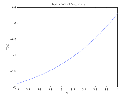
Figure 1. Dependence of $G(c_{l})$ on $c_{l}$ for $s=2$

	$s=2$	$s=3$	$s=4$	$s=5$
Linear Regression	$3.7942$	$3.3143$	$3.1718$	$3.0773$
Self-Similar Equations	$3.7967$	$3.3157$	$3.1597$	$3.0841$

Table 2. $c_{l}$ got from linear regression (6.10b) and the self-similar equations (1.6).

	$s=2$	$s=3$	$s=4$	$s=5$
Hölder exponent	$7.3381\times 10^{-1}$	$6.9823\times 10^{-1}$	$6.9131\times 10^{-1}$	$6.7610\times 10^{-1}$
$1-1/c_{l}$	$7.3661\times 10^{-1}$	$6.9841\times 10^{-1}$	$6.8351\times 10^{-1}$	$6.7576\times 10^{-1}$

Table 3. Hölder exponent of the velocity field at $0$ and $1-1/c_{l}$.

The self-similar profiles that are obtained from solving the self-similar equation (6.2) and from direct simulation of the model (6.11) are plotted in Figure 2. The lines labeled ‘exact’ are obtained from solving the self-similar equation (6.2). Others are obtained from rescaling the solution at different time steps corresponding to different maximal vorticity.(6.11)

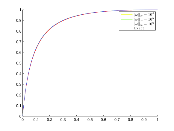
(a) The re-scaled solutions and self-similar profiles we construct. $s=2$.

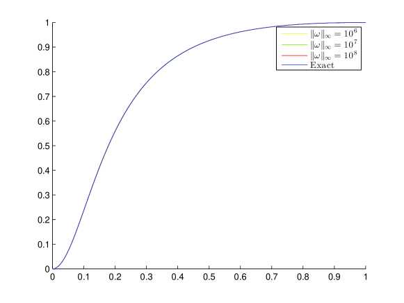
(b) The re-scaled solutions and self-similar profiles we construct. $s=3$.

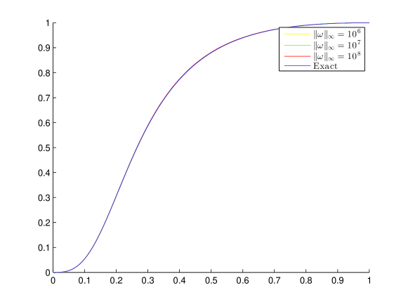
(c) The re-scaled solutions and self-similar profiles we construct. $s=4$.

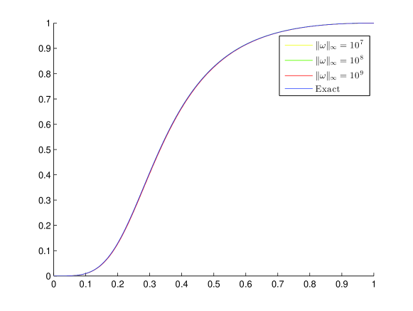
(d) The re-scaled solutions and self-similar profiles we construct. $s=5$.

Figure 2. Self-similar profiles of $w$ using initial condition $w(x,0)=1-\cos(4\pi x)$.

To demonstrate the stability the self-similar profiles, we consider another initial condition,

(6.19) $$w(x,0)=x-x^{2}.$$

The profiles obtained from rescaling the singular solutions (6.11) are plotted in Figure 3.

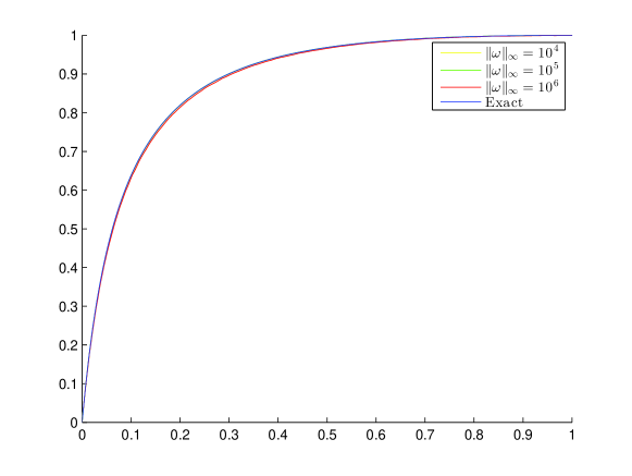
(a) $s=2$

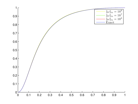
(b) $s=3$

Figure 3. Self-similar profiles of $w$ using initial condition $w(x,0)=x-x^{2}$.

From Figure 2, 3, we can see that after rescaling, the singular solutions at different time steps before the singularity time are very close, which implies that the solutions develop self-similar singularity. Besides, the self-similar profiles obtained from direct simulation of the model (6.11) agree very well with the self-similar profiles (6.2) we construct by sovling the self-similar equations (1.6). Moreover, for fixed leading order of $\theta(x,0)$ at the origin, the singular solutions with different initial conditions converge to the same set of self-similar profiles, which implies that the profiles have some stability property.

Remark 6.1.

If the initial leading order of $\theta(x,0)$ is $s\geq 3$, and a small perturbation of $\theta$, which we denote by $\epsilon\tilde{\theta}(x,t)$, has leading order $2\leq\tilde{s}<s$, then the profiles of the perturbed singular solutions will be determined by $\tilde{s}$, not $s$. From this point of view, only the self-similar profiles for $s=2$ are stable in the sense of perturbation.

7. Concluding Remarks

The existence of a discrete family of analytic self-similar profiles corresponding to different leading orders of the solutions at the origin for the CKY model has been established. The profiles are constructed using a power series method near the origin, and then extended to infinity by solving an ODE system. The decay condition in the Biot-Savart law determines the scaling exponents in the self-similar solutions. Numerical computation together with rigorous error estimation is used to prove the existence of these self-similar profiles. Far-field properties of the self-similar profiles are analyzed. The constructed self-similar profiles are consistent with direct simulation of the model and enjoy some stability property. The current method of analysis does not generalize directly to study the 3D Euler singularity. A new set of techniques are required to deal with the non-local Biot-Savart law. The existence of self-similar singularity for the 3D Euler equations is under investigation.

Acknowledgements. The authors would like to thank Professors Russel Caflisch and Guo Luo for a number of stimulating discussions. We would also like to thank Professors Alexander Kiselev and Yao Yao for their interest in our work and for their valuable comments. The research was in part supported by NSF FRG Grant DMS-1159138.

References

- [1] Kenneth Appel and Wolfgang Haken. Proof of 4-color theorem. Discrete Mathematics, 16(2):179–180, 1976.
- [2] Claude Bardos and Edriss Titi. Euler equations for incompressible ideal fluids. Russian Mathematical Surveys, 62(3):409, 2007.
- [3] Dongho Chae. Nonexistence of asymptotically self-similar singularities in the euler and the navier–stokes equations. Mathematische Annalen, 338(2):435–449, 2007.
- [4] Dongho Chae. Nonexistence of self-similar singularities for the 3d incompressible euler equations. Communications in Mathematical Physics, 273(1):203–215, 2007.
- [5] Dongho Chae. On the self-similar solutions of the 3d euler and the related equations. Communications in Mathematical Physics, 305(2):333–349, 2011.
- [6] Kyudong Choi, Thomas Y. Hou, Alexander Kiselev, Guo Luo, Vladimir Sverak, and Yao Yao. On the fiinite-time blowup of a 1d model for the 3d axisymmetric euler equations. arXiv preprint arXiv:1407.4776, 2014.
- [7] Kyudong Choi, Alexander Kiselev, and Yao Yao. Finite time blow up for a 1d model of 2d boussinesq system. arXiv preprint arXiv:1312.4913, 2013.
- [8] Earl A Coddington and Norman Levinson. Theory of ordinary differential equations. Tata McGraw-Hill Education, 1955.
- [9] Peter Constantin. On the euler equations of incompressible fluids. Bulletin of the American Mathematical Society, 44(4):603–621, 2007.
- [10] Charles L Fefferman and Luis A Seco. Interval arithmetic in quantum mechanics. In Applications of interval computations, pages 145–167. Springer, 1996.
- [11] Gerald B Folland. Introduction to partial differential equations. Princeton University Press, 1995.
- [12] D.J.H. Garling. Inequalities: a journey into linear analysis, volume 19. Cambridge University Press Cambridge, 2007.
- [13] John D Gibbon. The three-dimensional euler equations: Where do we stand? Physica D: Nonlinear Phenomena, 237(14):1894–1904, 2008.
- [14] Thomas C Hales. A proof of the kepler conjecture. Annals of mathematics, pages 1065–1185, 2005.
- [15] Thomas Y Hou and Guo Luo. On the finite-time blowup of a 1d model for the 3d incompressible euler equations. arXiv preprint arXiv:1311.2613, 2013.
- [16] R Baker Kearfott and Vladik Kreinovich. Applications of interval computations, volume 3. Kluwer Academic Dordrecht, 1996.
- [17] Alexander Kiselev and Vladimir Sverak. Small scale creation for solutions of the incompressible two dimensional euler equation. arXiv preprint arXiv:1310.4799, 2013.
- [18] Sof’ja V Kovalevskaja. Zur theorie der partiellen differentialgleichungen. 1874.
- [19] Oscar E Lanford III. A computer-assisted proof of the feigenbaum conjectures. Bulletin of the American Mathematical Society, 6(3):427–434, 1982.
- [20] Randall J LeVeque. Finite difference methods for ordinary and partial differential equations: steady-state and time-dependent problems, volume 98. Siam, 2007.
- [21] Guo Luo and Thomas Y Hou. Potentially singular solutions of the 3d incompressible euler equations. arXiv preprint arXiv:1310.0497, 2013.
- [22] Andrew J Majda and Andrea L Bertozzi. Vorticity and incompressible flow, volume 27. Cambridge University Press, 2002.
- [23] Dan Zuras, Mike Cowlishaw, Alex Aiken, Matthew Applegate, David Bailey, Steve Bass, Dileep Bhandarkar, Mahesh Bhat, David Bindel, Sylvie Boldo, et al. Ieee standard for floating-point arithmetic. IEEE Std 754-2008, pages 1–70, 2008.