Spectral atlases of the Sun from 3980 to 7100 Å
at the center and at the limb

Abstract

In this work, we present digital and graphical atlases of spectra of both the solar disk-center and of the limb near the Solar poles using data taken at the UTS$-$IAP & RIAAM (the University of Tabriz Siderostat, telescope and spectrograph jointly developed with the Institut d’Astrophysique de Paris and Research Institute for Astronomy and Astrophysics of Maragha). High resolution and high signal-to-noise ratio (SNR) CCD-slit spectra of the sun for 2 different parts of the disk, namely for $\mu$ = 1.0 (solar center) & for $\mu$ =  0.3 (solar limb) are provided and discussed. While there are several spectral atlases of the solar disk-center, this is the first spectral atlas ever produced for the solar limb at this spectral range. The resolution of the spectra is about R $\sim$ 70 000 ($\Delta\lambda$ $\sim$ 0.09 Å) with the signal-to-noise ratio (SNR) of 400$-$600. The full atlas covers the 3980 to 7100 Å spectral regions and contains 44 pages with three partial spectra of the solar spectrum put on each page to make it compact. The difference spectrum of the normalized solar disk-center and the solar limb is also included in the graphic presentation of the atlas to show the difference of line profiles, including far wings. The identification of the most significant solar lines is included in the graphic presentation of the atlas. Telluric lines are producing a definite signature on the difference spectra which is easy to notice. At the end of this paper we present only two sample pages of the whole atlas while the graphic presentation of the whole atlas along with its ASCII file can be accessed via the ftp server of the CDS in Strasbourg via anonymous ftp to cdsarc.u-strasbg.fr (130.79.128.5) or via this link .

Keywords atlases; sun: photosphere

1 Introduction

The existing solar atlases can be divided into two main categories: 1) solar full disk atlases (a.k.a solar flux or even irradiance atlases); 2) solar disk-center spectral atlases. A pioneering work of full disk solar atlases was the solar irradiance spectrum of Labs & Neckel (1968). This atlas covers a wide range of wavelengths but has a rather low spectral resolution such that even the major Fraunhofer lines were not resolved. It was not until 1976 that J. Beckers and his collaborators (Beckers et al. 1976) published the first high resolution solar flux atlas which covers the wavelength range of 3800 $-$ 7000 Å. Later on, Kurucz et al. (1984) used spectra taken at the McMath-Pierce Solar Telescope located on Kitt Peak Observatory, to publish their high resolution and high SNR solar flux atlas, covering the 2960 $-$ 13000 Å spectral region.

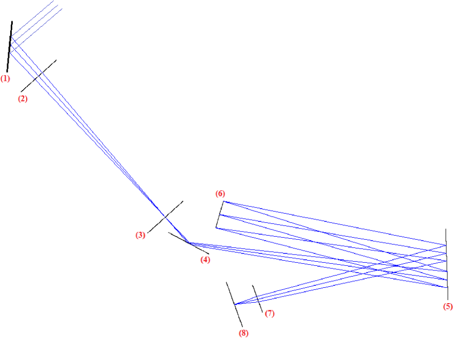
Fig. 1 : The optical layout of the instrument: 1) Siderostat primary 35 cm diameter plane mirror; 2) Zeiss astrograph F/15 objective with focal length of 3 m; 3) Adjustable slit; 4) Fold mirror 5) F/12 collimator with 30 cm diameter; 6) 16 cm Grating with 1800 grooves/mm and $\lambda_{blaze}$ $=$ 5500 Å; 7) Lens with 20 cm focal length; 8) The CCD.

The first widely used high resolution disk-center slit solar spectrum known as the Utrecht Spectrum was produced from photographic plates following a large effort by Minnaert et al. (1940) and many others. The original spectrograms were obtained at the 150- foot tower telescope of Mount Wilson in 1936-37. This atlas was later analyzed by Moore et al. (1966). Furthermore, the Liege and Jungfraujoch central intensity atlas, Spectrophotometric Atlas of the Solar Spectrum from $\lambda$3000 to $\lambda$10000 was published by Delbouille et al (1973). To obtain their photo-electric spectra recorded with several photo-multipliers to cover the whole spectral range, they repeatedly used a rapidly scanning large spectrometer fed by a coelostat at the high altitude Jungfraujoch station and selected the best digital recordings. This atlas is available by parts from the French BASS2000 ground-based solar data base. More recently, Wallace et al. (1998) published an atlas of the solar spectrum at disk center, based on archival Fourier transform spectrometer (FTS) data taken at the McMath-Pierce Solar Telescope. Several attempts were also made by Amateurs to produce a compact atlas more limited in quality but more practical .

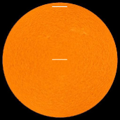
Fig. 2 : The positions of the slit on the solar disk. The two while lines show the positions of the slit at the solar disk-center ($\mu$ = 1.0) and on the solar limb ($\mu$ = 0.3).

In the current work, we present an atlas of the solar disk-center ($\mu$ = 1.0) of the quiet Sun along with that of the solar limb ($\mu$ = 0.3) and make a comparison. Spectra are based on data taken at the University of Tabriz Siderostat developed in cooperation with the Institut d’Astrophysique de Paris (UTS$-$IAP) in 2000 - 2005. Noting that very large telescopes today are capable of producing rather good resolution spectra, even for far objects, we hope this atlas along with its companion ASCII file would contribute to researches in solar, interplanetary, cometary, stellar, galactic and extra-galactic physics. We note that this atlas is the first of a series of atlases. The future atlases will cover the near-infrared part of the spectrum and even more importantly and more difficult to produce spectra of the core of a solar sunspot (work in progress).

2 Set-up and Observations

To make the current atlas we use the UTS-IAP solar telescope and spectrograph (see the optical layout of the instrument in Fig. 1). The grating has 1800 grooves per millimeter with the blaze wavelength at 5500 Å. Our spectrograph is in the Ebert-Fastie configuration and the 30 cm diameter F/12 collimator is used for both collimating and focusing the incident light. As illustrated in Fig. 1, the light of the sun enters the spectrograph via the objective lens, after first striking the siderostat primary 35 cm diameter plane mirror. The focal length of the Zeiss astrograph F/15 objective is 3 m, and the slit width of the spectrograph is fixed at 20 $\mu$m which gives us a resolution of R $\sim$ 70 000. The sunlight passes through the slit and strikes the collimator located at 3.7 m away. The collimated beam of light then hits the grating which is also 3.7 m away from the collimator. The grating disperses the light into a 1st order spectrum and then reflects it back on the collimator. The collimator is now focussing the dispersed light on the CCD chip. We emphasize that, in order to increase the wavelength coverage of the CCD chip, we equipped the CCD with a lens of 20 cm focal length to slightly demagnify (see below). Table 1 reports the date of observation, solar altitude and humidity at the time of observations.

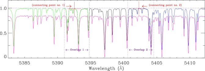
Fig. 3 : An illustration of the procedure used to juxtapose all individual observed spectral windows. The green, black and blue curves are the three spectral windows that are to be combined. The two red crosshairs mark the positions of the two connecting points and the pink curve is the final combined spectrum. For the sake of comparison, the final spectrum (i.e. the pink curve) is shifted along the y-axis.

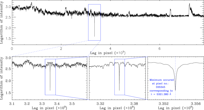
Fig. 4 : A cross-correlation of an observed spectral window and the KPNO spectrum. The position of the minimum corresponds to the lag at which the two spectra overlap the most. This lag is then used to do wavelength calibration on the observed spectrum.

We used an Atik ATK-2HS CCD camera to record the observed 2$-$dimensional (2D) spectral images. The CCD chip is of 640$\times$480 pixels, that is 640 pixels along the dispersion axis and 480 pixels along the slit. The width and the length of the slit covers $\sim$ 1.4 and $\sim$ 75 arcsecond on the solar surface, respectively. Sunspots and pores were avoided and no faculae were seen at the polar limb during the used recordings. Fig 2 shows the two different positions of the slit on the solar disk. In this figure, the two white lines indicate the positions of the slit. In a single exposure, the 640 pixels along the dispersion axis could only cover 11 to 15 angstroms of the solar spectrum. Therefore, we required more than 330 separate 2D spectral images to cover the whole spectral range of interest. These spectral segments are extracted and then assembled to form the final atlas. We note that each of these 2D images has about 3 to 5 angstrom overlap with its successive images. These overlaps are then used to juxtapose all the individual exposures in order to make one single spectrum that ranges from 3980 to 7100 Å. To this end, each spectral window is plotted with its two neighboring windows over-plotted on it with different colors (see Fig. 3). We then interactively mark two appropriate connecting points (away from the troughs of the absorption lines), one for each neighboring window. The three successive spectra are then combined by averaging the intensity of each of the two overlapping windows at their corresponding connecting points. This is done for all the observed spectral windows. In Fig. 3, the two red crosshairs indicate the positions of the two connecting points. The final combined spectrum is also shown as a pink curve. Note that for the sake of comparison, the y-axis of the final combined spectrum (i.e. the pink curve) is shifted along the y-axis.

As for the Atlas (called KPNO hereafter) we compare our work with, the spectrum (Wallace et al. 1998) was recorded using a Fourier Transform Spectrometer (FTS; Davis et al. 2001). The solar image from the large Kitt-Peak siderostat tower telescope of 1.6 m aperture is focused on a rotating vertical table at the entrance aperture of the FTS. These apertures are circular and their diameter ranges from 0.5 mm (1.2 arcsec) to 10 mm (25 arcsec). The final spectrum is then obtained by computing the Fourier transform of the recorded interferograms. It usually takes 3 to 14 minutes to complete a single, full resolution scan. Several of such scans are generally taken in order to improve the SNR of the interferograms.

Table 1 : Observing condition at the time of observation. Note that the observations were done in 2013 in rather different conditions for Earth atmospheric transmission.

	Date of Obs.	Solar altitude	Humidity
Solar Center	June 7 & 8	70 o	30 %
Solar Limb	Nov. 18 & 19	30 o	55 %

3 The Wavelength Calibration

Each spectral window was wavelength-calibrated separately. We used a new method for doing the wavelength calibration. What is usually done in spectroscopy is to take spectra of calibration lamps (ex. Th-Ar; He-Ne lamps) with the same setup that the object spectra were obtained with. However, if obtaining on-board calibration data is not possible (ex. in the case of spectra recorded by SUMER spectrograph mounted on SoHO space telescope) wavelength calibration is done with the help of some stable photospheric spectral lines (Vial et al. 2007). But in the current work, we use cross-correlation analysis in order to do wavelength calibration on our observed spectra. Cross-correlation analysis is the most popular procedure for deriving relative velocities between an observed stellar spectrum and a template spectrum (Tonry & Davis 1979). We note that, in this work, the solar spectrum observed by Wallace et al. (1998) (i.e. KPNO spectrum) is used as the template spectrum for our cross-correlation analysis.

A cross-correlation measures the similarity between two signals. For this purpose, the whole KPNO spectrum is searched for the pattern similar to that of the observed spectral window. To this end, the observed spectrum is shifted iteratively with respect to the KPNO spectrum by a series of regularly spaced increments. We then compute the sum of the normalized flux differences of the shifted and unshifted spectrum at each pixel. The output of the cross-correlation between one sample observed spectrum and the KPNO spectrum is shown in Fig. 4. In this figure, the position of the cross-correlation minimum (i.e. pixel no. 335345) corresponds to the lag between the two spectra.

As noted in sect. 2, our CCD has 640 pixels along the dispersion axis while the KPNO spectrum, for the same wavelength range, contains $\sim$ 1000 (in the red part of the spectrum) up to $\sim$ 5000 (in the blue part of the spectrum) data-points. Therefore, before cross-correlating the two spectra, each observed spectral window is re-sampled to match the KPNO spectrum wavelength grid.

4 Instrumental profile

Telluric lines, especially those of the molecular oxygen bands are much narrower than solar absorption lines, and their profiles can provide an indication of the instrumental profile of the spectrograph (Griffin 1969). Fig. 5 presents the absorption profiles of the telluric $\alpha$ -band (upper panel) and B-band (lower panel) of oxygen taken from the current atlas. To distinguish between the telluric and solar absorption in this region, we put a blue vertical tick below each solar absorption line. In the upper panel of Fig. 5, the two lines marked by the green stars are the two absorption used in determining the instrumental profile of the spectrograph (see below).

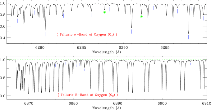
Fig. 5 : The absorption profiles of the telluric $\alpha$ -band (upper panel) and B-band (lower panel) of oxygen taken from the current atlas. The absorption lines marked by the blue vertical ticks are solar. In the upper panel, the two lines marked by the green stars are the two absorption lines used in determining the instrumental profile of the spectrograph.

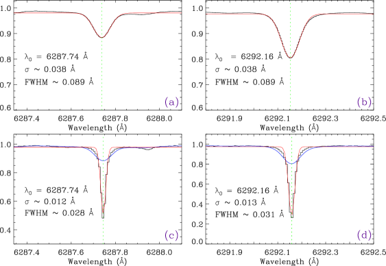
Fig. 6 : The two absorption lines of the telluric $\alpha$ band of oxygen with $\lambda$ $\sim$ 6287.74 Å and $\lambda$ $\sim$ 6291.16 Å are used to compare the instrumental profiles of the current atlas (panels (a) and (b)) with that of the Wallace et al. (1998) (panels (c) and (d)). A Gaussian fit (red curve) is conducted on each of the individual absorption line (black curves) to determine the Gaussian width ($\sigma$) as well as the FWHM of the line. Note that in panels (c) and (d), for the ease of comparison, the corresponding telluric lines of the current atlas are also shown as blue curves.

We compare, in Fig. 6, the instrumental profile of the current atlas with that of the KPNO spectrum. For this purpose, we conducted Gaussian fits (red curves) to two absorption lines (black curves) of the telluric $\alpha$ band of Oxygen, namely, the ones at $\lambda$ $\sim$ 6287.74 Å and $\lambda$ $\sim$ 6291.16 Å. The upper two panels in Fig. 6 (i.e. panels (a), and (b)) are for the current atlas while the lower two panels belong to the KPNO spectrum. Moreover, in each panel, we report the central wavelength of the profile ($\lambda_{0}$), the Gaussian width ($\sigma$), and the FWHM of the absorption lines. Note that in panels (c) and (d), for the ease of comparison, the corresponding telluric lines of the current atlas are also shown as blue curves.

The FWHM of the two telluric absorption lines of the current atlas (panels (a) and (b) in Fig. 6) are $\sim$ 0.09 Å, resulting in a resolving power of R = $\lambda$/$\Delta\lambda$ $\sim$ 70 000. At this R, the spectral resolution bin of $\Delta\lambda$ $\sim$ 0.09 is sampled by four detector pixels (i.e. each pixel of 7.4 $\mu$m length covers $\sim$ 0.02 Å.). On the other hand, in the KPNO spectrum (panels (c) and (d)), the FWHM of  $\sim$ 0.03 Å yields a resolving power of  $\sim$ 210 000.

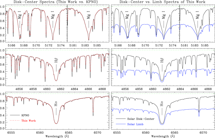
Fig. 7 : Comparing the line profiles of H $\alpha$, H $\beta$, and Mg I triplet of the KPNO spectrum and those of the current work. In the left-hand side panels, the solar disk-center spectrum of the KPNO (black curves) is compared with that of the current work (red curves). In the right-hand side panels, on the other hand, our solar disk-center (black curves) and solar limb (blue curves) spectra are compared. We note that, in the case of the limb spectra, the level of the continuum was normalized to the values given in Allen (1981).

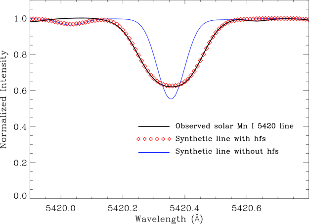
Fig. 8 : A demonstration of the effect of hyperfine structure on the Mn i absorption profile observed with the UTS$-$IAP spectrograph. This is the same as Figure 3.1 of Gray (2010) but reproduced using our own observed solar spectrum.

5 Discussion

The spectra used for the current work were taken at the solar disk-center with $\mu$ = 1.0 and the solar limb with $\mu$ = 0.3. We tried to avoid plage, sunspots and active regions during our observations. The quality of the spectrum is high as the achieved SNR is 400-600, thanks to the integration performed along the slit. The final atlas, ranging from 3980 to 7100 Å, contains 44 pages of graphic presentation of the spectrum with the identification of most of the lines included. Each page contains 3 partial spectra. The identification of lines is made using the reference atlas of Moore et al. (1966). Two sample pages of the whole atlas are shown at the end of this paper. Each page contains three spectral windows, with each window made up of two panels. The upper panel shows the spectrum of the solar disk-center (black curve) on which the spectrum of the solar limb is overplotted as the red curve while the lower panel illustrates the difference spectrum of the two (i.e. I($\mu$ = 1.0) $-$ I($\mu$ = 0.3)). The difference spectrum of the lower panel clearly indicates that the absorption lines taken at the solar disk-center are usually deeper than those taken at the solar limb (in this panel the two pink dashed lines indicate the residual intensity of 0.05 above and below zero). Note that, in the solar limb spectrum, the level of the continuum was put to the reference level given in the Astrophysical Quantities, 3rd Edition by C. W. Allen, p. 169. Moreover, the ASCII file of the atlas is also provided as a companion to this paper.

In Fig. 7, the absorption profiles of H $\alpha$, H $\beta$, and Mg I triplet of the KPNO spectrum and current atlas are presented and compared. In this figure, in the left-hand side panels, the solar disk-center spectrum of the KPNO (black curves) is compared with that of the current work (red curves). In the right-hand side panels, on the other hand, our solar disk-center (black curves) and solar limb (blue curves) spectra are compared. As illustrated in this figure, the wings of the Balmer lines (i.e. H $\alpha$ and H $\beta$) are narrower at the solar limb than they are at the solar disk-center.

In central ($\mu$ = 1) intensity, the continuum is formed at about 5500 K while in the case of $\mu$ = 0.3, we do not see as far in, instead, we only see down to 5000 K or so where the continuum is less bright (Vernazza et al. 1981). Moreover, the line wings are produced by Stark broadening which is proportional to the electron number density (Gray 2008). Inspecting the Kurucz Solar atmosphere model (Kurucz 1993) at T $\sim$ 5500 and 5000 K shows that the electron number density is lower for the latter temperature. Therefore, the lower electron number density can result in a lower amount of Stark broadening, and hence narrower wings, as seen for the Balmer lines in Fig. 7. In this figure, the center-limb variations of intensities of the Balmer lines show a limb darkening effect whatever the position in the line, as has been established for a long time (Dunn, 1959; White, 1962). We note that, in Fig.7, in the case of the limb spectra, the level of the continuum was normalized to the values given in Allen (1981).

As shown in Table 1, during the solar limb observation, the humidity was higher than when the solar disk-center data were being recorded. As a result, the features seen in the difference spectrum for the telluric lines are all above zero, making them easy to identify. Needless to say, the lower altitude of the sun during the solar limb observation also had some contribution to this effect.

Finally, we want to point out that the quality of our compacted digital spectra is sufficient to make a research quality work using the recorded line profiles. The width of chromospheric lines is readily recognized. Indeed, there are several photospheric absorption lines in the observed solar spectrum that are unusually broad; a simple Gaussian or Voigt profile fit cannot reproduce the observed profile (see Fig. 8). To model these absorption profiles, we have to take into account the hyperfine structure of atoms we are studying. In Fig. 8, we demonstrate the effects of the hyperfine structure on the Mn i 5420 Å absorption line. In this figure, the observed spectrum is shown as the solid black line, the synthetic spectrum without hyperfine structure taken into account is shown as the blue line, and the red squares show the synthetic spectrum with hyperfine structure taken into account. The synthetic profiles were constructed using SPECTRUM v2.67 code developed by Richard O. Gray (Gray & Corbally, 1994). We note that Fig. 8 is the same as Figure 3.1 of Gray (2010) but reproduced using our own observed solar spectrum.

Acknowledgements We would like to thank the anonymous referee for his/her careful reviews of the paper that include many important points and improved significantly the clarity of the paper. HFV would like to thank Prof. Patrick Petitjean, Prof. Robert Kurucz, Dr. Hossein Ebadi and Dr. Hadi Rahmani for their useful discussion. This work has been financially supported by the Research Institute for Astronomy and Astrophysics of Maragha (RIAAM) under research project No. 1/312. Part of this work is made in the frame of the Iran- France Programme Hubert Curien (PHC) ”Gundishapur” of scientific exchanges initiated by the University of Tabriz and the Institut d’Astrophysique de Paris. NSO/Kitt Peak FTS data used here were produced by NSF/NOAO.

References

- Allen (1981) Allen, C. W., 1981, ”Astrophysical Quantities”, 3rd edition, The Athlone Press, The University of London, London
- Beckers et. al. (1976) Beckers, J. M., Bridges, C. A., & Gilliam, L. B., 1976, ”A High Resolution Spectral Atlas of the Solar Irradiance from 380 to 700 Nanometers”, Hanscom AFB: Sacramento Peak Obs
- Davis et al. (2001) Davis, S. P., Abrams, M. C., Brault, J. W., 2001, ”Fourier transform spectrometry”, San Diego, Calif. : Academic Press
- Delbouille (1973) Delbouille, L., Roland, G., & Neven, L., 1973, ”Photometric Atlas of the Solar Spectrum from 3000 to 10000”, Liege: Inst. d’Ap., Univ. de Liege
- dunn (1959) Dunn, R. B.: ApJ, 130, 972 (1959)
- gray (2008) Gray, D.F. 2008, ”The Observation and Analysis of Stellar Photospheres”, 3rd edition, Cambridge, Cambridge University Press
- gray (2010) Gray, R. O., 2010, ”Documentation for SPECTRUM v2.76”
- gray et al. (1994) Gray, R. O., Corbally, C. J.: AJ, 107, 742 (1994)
- Griffin (1979) Griffin, R. F.: MNRAS, 143, 361 (1969)
- Kurucz (1993) Kurucz, R. L. 1993, CD-ROM 13, atlas9 Stellar Atmosphere Programs and 2 km/s Grid (Cambridge: Smithsonian Astrophys. Obs.)
- Kurucz et. al. (1984) Kurucz, R.L., Furenlid, I., Brault, J., & Testerman, L., 1984, ”Solar Flux Atlas from 296 to 1300 nm”, New Mexico: National Solar Observatory
- Minnaert et. al. (1940) Minnaert, M., Houtgast, J., & Mulders, G.F.W., 1940, ”Photometric atlas of the solar spectrum from 3612 to 8771 with an appendix from 3332 to 3637”, Sterrewacht ”Sonnenborgh”, Utrecht
- Moore et. al. (1966) Moore, C. E., Minnaert, M. G. J., & Houtgast, J., 1966), ”The Solar Spectrum 2935 Å to 8770 Å”, NBS Monograph Vol. 61, Washington, DC: US GPO
- tonry et al. (1979) Tonry, J., Davis, M.: AJ, 84, 1511 (1979)
- Vernazza et al. (1981) Vernazza, J. E., Avrett, E. H., Loeser, R.: ApJS, 45, 635 (1981)
- Vial et al. (2009) Vial, J.-C., Ebadi, H., Ajabshirizadeh, A.: Sol. Phys. 246, 327 (2007)
- Wallace et al. (1998) Wallace, L., Hinkle, K., & Livingston, W., 1998, ”An atlas of the spectrum of the solar photosphere from 13,500 to 28,000 cm-1 (3570 to 7405 Å)”, ed.Wallace, L., Hinkle, K., & Livingston, W
- white (1962) White, O. R.: ApJS, 7, 333 (1962)