First-principles DFT+GW study of oxygen vacancies in rutile TiO₂

Abstract

We perform first-principles calculations of the quasiparticle defect states, charge transition levels, and formation energies of oxygen vacancies in rutile titanium dioxide. The calculations are done within the recently developed combined DFT+GW formalism, including the necessary electrostatic corrections for the supercells with charged defects. We find the oxygen vacancy to be a negative $U$ defect, where $U$ is the defect electron addition energy. For the values of Fermi level below $\sim 2.8$ eV (relative to the valence band maximum) we find the $+2$ charge state of the vacancy to be the most stable, while above $2.8$ eV we find that the neutral charge state is the most stable.

I Introduction

Titanium dioxide (TiO₂) attracts a lot of attention of researchers as a versatile functional material used in numerous technological applications including photocatalysis, hydrolysis, solar cells, high-$k$ dielectrics, optoelectronic devices, sensors, etc. Grant (1959); Diebold (2003); Augustynski (1993); Linsebigler et al. (1995); O’Regan and Grätzel (1991); Yang et al. (2008); Kim et al. (2008); Wilk et al. (2001); Fujishima and Honda (1972) Lattice defects, such as vacancies, substitution impurities, and interstitial impurities, inevitably occur in materials regardless of whether they are synthesized or created naturally. These defects can greatly influence the mechanical, electrical, thermal, and optical properties of solids.

Among the major three crystal polymorphs of TiO₂, rutile is the most common one, the other two being anatase and brookite. Rutile TiO₂ has a tetragonal primitive cell with two formula units (see Fig. 1) and its symmetry is described by the space group $P4_{2}/mnm$. The lattice parameters are $a=4.594$ Å and $c=2.959$ Å at room temperature. The Ti and O atoms reside at the $2a$ and $4f$ Wyckoff positions, the latter characterized by the single internal parameter $u=0.305$.Abrahams and Bernstein (1971)

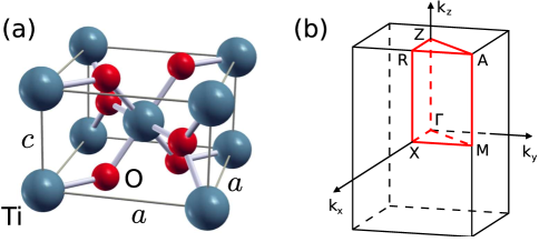
Figure 1: (Color online.) (a) Tetragonal primitive cell of TiO₂ in the rutile crystal structure. (b) The corresponding Brillouin zone.

Rutile TiO₂ in its stoichiometric form is an insulator with an optical band gap of $3.0$ eV.Cronemeyer (1959); Amtout and Leonelli (1995) The optical gap, however, is smaller than the electronic band gap due to electron-hole interactions. The latter band gap is connected to a single-particle (or quasiparticle) description and can be measured in photoemission experiments. The values for the electronic gap in the literature vary in the range of $3.3-4.0$ eV. Tezuka et al. (1994); Hardman et al. (1994); Rangan et al. (2010) For more discussion on the relation between the electronic and optical gaps of TiO₂, as well as comparison of experimental and theoretical values, see, e.g., Ref. Chiodo et al., 2010.

Heating rutile crystals in reducing atmosphere results in the increase of the ($n$-type) electrical conductivity and rutile composition changes to non-stoichiometric TiO_2-x. This change is attributed to various types of defects such as oxygen vacancies, Ti³⁺ and Ti⁴⁺ interstitials, and planar defects.Diebold (2003)

In this work we perform calculations of the charge transition levels and defect formation energies of oxygen vacancies in three charge states following a recently developed DFT+GW approach.Hedström et al. (2006); *rinke_09; Jain et al. (2011) There are several advantages of this approach over the traditional DFT-only approaches.Iddir et al. (2007) In this method, the GW correction of DFT eigenvalues takes care of the self-energy and self-interaction errors and resolves the problem of band-gap underestimation. The latter problem is often responsible for incorrect DFT prediction of defect level position outside the bulk band gap. In addition, within the DFT+GW approach the formation energies can be calculated without computing differences in total energies of systems with different number of electrons. We note that the need to go beyond the standard DFT approaches for calculations of defect formation energies and charge transition levels is now well recognized, as more studies of the electronic structure of oxides based on hybrid functionals and GW perturbation methods appear in the literature. Recently, Peng and collaboratorsPeng et al. (2013) proposed an alternative scheme to calculate defect formation energies by using GW to correct band edge energies.

The rest of the paper is organized as follows. Section II describes in detail the DFT+GW formalism used in our calculations. Computational details are given in section III. Then the main results are presented in section IV, followed by a summary in section V.

II Methods

II.1 DFT+GW formalism

The DFT+GW approach employed in this work is developed in Refs. Hedström et al., 2006; *rinke_09 and Jain et al., 2011. Here, we will introduce the notations used in the subsequent sections.

We describe the atomic state of a system with defect in a charge state $q$ (oxygen vacancy $V_{\mathrm{O}}^{q}$ in our case) by a generalized coordinate $\mathbf{R}$. In general, $\mathbf{R}$ corresponds to an arbitrary configuration, not necessarily equilibrium configuration. The equilibrium configuration of the defect in a charge state $q$ we will denote as $\mathbf{R}_{q}$. One can defineJain et al. (2011) the defect formation energy $E^{\mathrm{f}}_{q}(\mathbf{R},\mu_{\mathrm{O}},E_{\mathrm{F}})$, which depends on the chemical potential of oxygen $\mu_{\mathrm{O}}$ (determined by the experimental preparation conditions) and the Fermi level $E_{\mathrm{F}}$. We reference $E_{\mathrm{F}}$ to the valence band maximum (VBM), so it can take values between zero and the bulk band gap depending on the specific sample.

Charge transition level $\epsilon^{q/q-1}$ is defined as the Fermi level at which the charge state of the defect changes from $q$ to $q-1$ or, in other words, at which the formation energies of the defect in charge states $q$ and $q-1$ are equal. One can show that the value of the charge transition level can be separated into two contributions as $\epsilon^{q/q-1}=E_{\mathrm{relax}}+E_{\mathrm{QP}}$, where $E_{\mathrm{QP}}$ is a quasiparticle excitation energy (addition or removal of a single electron) and $E_{\mathrm{relax}}$ is the (atomic) relaxation energy of the defect in the new charge state. Since $E_{\mathrm{relax}}$ is given by the difference in the total energies of the system whose total number of electrons remains unchanged, it can be calculated accurately using standard DFT methods, while $E_{\mathrm{QP}}$ may be evaluated using the ab initio GW method.Hybertsen and Louie (1986)

The combined DFT+GW approach avoids the typical problems one encounters when using DFT for all terms, such as the underestimation of the band gap and self-interaction errors.

II.2 Electrostatic corrections

Ideally, when studying defects, one would like to consider a single defect in an infinite bulk material. In practice, however, one often uses a supercell approach,Cohen et al. (1975) in which a finite supercell with defect is constructed and periodic boundary conditions are applied. If the supercell is not large enough the spurious interactions between the defect and its own images should be taken into account. For charged defects, in particular, the spurious long-range Coulomb potential from defect images results in a shift of the defect state in the bulk band gap. This effect has been shown to be quite significant for oxygen vacancies in hafnia.Jain et al. (2011)

There are several ways to calculate the electrostatic corrections, to be denoted as $\Delta{E}_{\mathrm{QP}}^{\mathrm{e.s.}}$. All of them can be done withing the DFT-only formalism since the spurious potential is electrostatic and affects only the Hartree potential in the DFT calculation. Further, Hartree potential is not affected by the self-energy operator within our GW approach. The straightforward approach would be to increase the size of the supercell with defect and keep track of the shift in the Kohn-Sham eigenvalue corresponding to the defect state. Taking into account the fact that the strength of the Coulomb interaction is inversely proportional to the distance, one can extrapolate the change in the Kohn-Sham eigenvalue to infinite supercell size.Jain et al. (2011) This approach, however, requires construction of supercells with very large number of atoms (often thousands of atoms are required).

In this work, we opted for a different approach proposed by Freysoldt and collaborators,Freysoldt et al. (2009) which does not require a construction of extremely large supercells. The only requirement on the supercell size is that the charge density associated with the defect state is well localized in a small volume inside the supercell. In the following, we describe the main changes to this method adapting it to DFT+GW framework. We shall keep the original notations and definitions.

If a neutral defect state can be described by a local wavefunction $\psi_{\mathrm{d}}$ then one can calculate the unscreened charge density $q_{\mathrm{d}}(\mathbf{r})$ associated with the charged defect (assuming the charge $q$ goes entirely to the local defect state). The charge $q$ then becomes screened by the surrounding electrons. The corresponding change in the electrostatic potential relative to the neutral defect is denoted by $V_{q/0}$. Note that in this discussion, as in the original formulation,Freysoldt et al. (2009) we do not consider effects of lattice relaxations due to the change of the charge state of the defect.

Now we consider a periodic system corresponding to an array of charged defects and add a compensating homogeneous background charge with density $n=-q/\Omega$, where $\Omega$ is the supercell volume. Assuming a linear-response behavior, the change in the electrostatic potential for this system $\widetilde{V}_{q/0}(\mathbf{r})$ is given by a superposition of the potentials $V_{q/0}(\mathbf{r}+\mathbf{R})$ up to a constant, where $\mathbf{R}$ denotes lattice vectors. Thus, knowing $V_{q/0}(\mathbf{r})$ of an infinite system one can reproduce the potential $\widetilde{V}_{q/0}(\mathbf{r})$ of a periodic system (up to a constant). The spurious electrostatic potential induced by the images of the defect in the home supercell is, thus, given by $[\widetilde{V}_{q/0}(\mathbf{r})-V_{q/0}(\mathbf{r})]$. Within DFT, this corresponds to the undesired shift of the Kohn-Sham defect state

$$\Delta\epsilon^{\mathrm{KS}}_{\mathrm{d}}=-\int_{\Omega}d^{3}r\,|\psi_{\mathrm{d}}(\mathbf{r})|^{2}[\widetilde{V}_{q/0}(\mathbf{r})-V_{q/0}(\mathbf{r})].$$ (1)

In practice, we can compute the periodic potential $\widetilde{V}_{q/0}(\mathbf{r})$ but we do not know the original potential $V_{q/0}(\mathbf{r})$ of the infinite system. At large distances this potential may be well approximated by the long-range screened Coulomb potentialFreysoldt et al. (2009) $V_{q/0}^{\mathrm{lr}}(\mathbf{r})$, which requires knowledge of the dielectric constant $\varepsilon$ (which, in turn, can be found, e.g., from density-functional perturbation theory) for its evaluation. Thus, the idea is to separate the potential $V_{q/0}(\mathbf{r})$ into long-range and short-range parts as $V_{q/0}(\mathbf{r})=V_{q/0}^{\mathrm{lr}}(\mathbf{r})+V_{q/0}^{\mathrm{sr}}(\mathbf{r})$. Assuming that the short-range potential decays rapidly with distance and is essentially zero at the border of the supercell (with defect placed in the center of the supercell), we can write for $\mathbf{r}\in\Omega$

$$\widetilde{V}_{q/0}^{\mathrm{sr}}(\mathbf{r})=V_{q/0}^{\mathrm{sr}}(\mathbf{r})+C,$$ (2)

where the constant $C$ absorbs the ambiguity in the absolute position of $\widetilde{V}_{q/0}$. This constant may be found by requiring that $\widetilde{V}_{q/0}$ and $\widetilde{V}_{q/0}^{\mathrm{lr}}$ align far from the defect.

Hence, the shift of the defect state due to the spurious electrostatic potential, Eq. (1), can be calculated from two parts, each coming from the long-range and short-range contributions to the potential. The first part is given by

$$\Delta\epsilon^{\mathrm{KS}}_{\mathrm{d},\mathrm{lr}}=-\int_{\Omega}d^{3}r\,|\psi_{\mathrm{d}}(\mathbf{r})|^{2}[\widetilde{V}_{q}^{\mathrm{lr}}(\mathbf{r})-V_{q}^{\mathrm{lr}}(\mathbf{r})]$$ (3)

and the second part is given by

$$\Delta\epsilon^{\mathrm{KS}}_{\mathrm{d},\mathrm{sr}}=-\int_{\Omega}d^{3}r\,|\psi_{\mathrm{d}}(\mathbf{r})|^{2}[\widetilde{V}_{q/0}^{\mathrm{sr}}(\mathbf{r})-V_{q/0}^{\mathrm{sr}}(\mathbf{r})]=-C.$$ (4)

Equations (3) and (4) give the spurious shift of the Kohn-Sham level, while the electrostatic correction $\Delta{E}^{\mathrm{e.s.}}_{\mathrm{QP}}$ that needs to be applied is

$$\Delta{E}^{\mathrm{e.s.}}_{\mathrm{QP}}=-\Delta\epsilon^{\mathrm{KS}}_{\mathrm{d},\mathrm{lr}}-\Delta\epsilon^{\mathrm{KS}}_{\mathrm{d},\mathrm{sr}}.$$ (5)

To see how the described above method works, we performed a calculation of the oxygen vacancy in rock-salt MgO in its $+1$ charge state. For simplicity, we performed a spin unpolarized calculation using $2\times 2\times 2$ cubic supercelli (63 atoms). We found a Kohn-Sham eigenvalue in the bulk band gap corresponding to a defect state located $1.07$ eV above the VBM. The electrostatic correction calculated with the above method resulted in a shift of defect eigenvalue of $-0.65$ eV, where $-0.45$ eV comes from the first term in Eq. (5) and $-0.20$ eV comes from the second term. Then, we performed calculations using $3\times 3\times 3$ (215 atoms) and $4\times 4\times 4$ (511 atoms) supercells. We found the defect eigenvalue to be $0.83$ eV and $0.64$ eV above VBM in 215-atom and 511-atom supercells, respectively. We fit the defect eigenvalue to $\epsilon_{d}=\epsilon_{d}^{0}+A/(L)$, where $L$ is the size of the supercell in arbitrary units (e.g., $L=2,3,4$ in our case), $\epsilon_{d}^{0}$, and $A$ are fitting parameters. This way, we found, in the limit of infinite supercell, the electrostatic correction to be $-0.84$ eV in a reasonable agreement with the previous result.

Recently, a similar procedure for correcting the Kohn-Sham eigenvalues due to electrostatic spurious potential was suggested by Chen and Pasquarello. Chen and Pasquarello (2013)

III Computational details

In this work all mean field calculations were done within the density functional theory (DFT) framework. It has been shown recently that structural relaxation in the case of rutile TiO₂ depends strongly on the choice of exchange-correlation potential.Janotti et al. (2010) Adequate description of the crystal structure can be obtained using hybrid functionals, such as that of Heyd, Scuseria, and Ernzerhof (HSE).Heyd et al. (2003); *heyd_06 If the crystal structure of rutile TiO₂ with oxygen vacancy is relaxed, e.g., using the Perdew, Burke, and Ernzerhof (PBE) exchange-correlation potential,Perdew et al. (1996) the defect level moves into conduction band regardless of its charge state.Janotti et al. (2010) For this reason, in our work, all structural relaxations (both for bulk TiO₂ and supercells with defects) were performed using HSE06 hybrid functional,Heyd et al. (2003); *heyd_06 in which 25% of the (short-range) Hartree-Fock (HF) exchange is mixed with 75% PBE exchange. We used projector augmented-wave (PAW) method Blöchl (1994); Kresse and Joubert (1999) as implemented in the VASP code package.Kresse and Furthmüller (1996a); *VASP2 The standard PBE pseudopotentials for both Ti and O supplied with the VASP package were employed. For Ti, the $3s$, $3p$, $3d$, and $4s$ states were treated as valence orbitals. We used a plane-wave basis set with an energy cut-off of 450 eV.

For bulk TiO₂, the Brillouin zone was sampled by a uniform $4\times 4\times 6$ $k$-point mesh. Oxygen vacancies were simulated by constructing a $2\times 2\times 3$ supercell of 72 atoms and removing one O atom. Brillouin zone integrations for the supercells were performed using an equivalent $2\times 2\times 2$ mesh of $k$ points.

Once the structural parameters for a system of interest were determined, we performed a separate self-consistent field (SCF) calculation using PBE exchange-correlation potential in order to obtain a mean-field starting point for our GW calculations. For this purpose we used Quantum ESPRESSO code package.Giannozzi et al. (2009) Troullier-Martins norm-conserving pseudopotentialsTroullier and Martins (1991) were generated for Ti and O. For Ti, the $3s$ and $3p$ semi-core states were treated as valence and the pseudopotential was generated in the Ti⁴⁺ configuration. The cut-off radii for the $3s$, $3p$, and $3d$ states were chosen to be $0.9$, $0.9$, and $1.0$ a.u., respectively. The energy cut-off for the plane-wave basis of 200 Ry was used in this case.

The GW calculations were performed using the BerkeleyGW code package.Hybertsen and Louie (1986); Deslippe et al. (2012) We used a G₀W₀ approach within the complex generalized plasmon-pole (GPP) model.Zhang et al. (1989) For the dielectric matrix calculation, the frequency cut-off was chosen to be 40 Ry and the number of valence and conduction bands was chosen to be 2 000 for bulk rutile TiO₂ and 4 000 for the supercell calculations. In case of supercells, the convergence with respect to empty states is not guaranteed despite the large number of states used in our calculations. For this reason, the extrapolation to infinite number of states is required. We used the static-remainder method for this purpose.Deslippe et al. (2013)

IV Results

IV.1 Bulk rutile TiO₂

Structural properties of bulk rutile TiO₂ were calculated using both PBE and HSE06 exchange-correlation potentials. The results of these calculations are in a very good agreement with each other and experiment as can be seen from Table 1.

Table 1: Calculated and experimental structural parameters of rutile TiO₂.

	$a$	$c/a$	$u$
	(Å)
PBE	4.64	0.639	0.305
HSE06	4.58	0.646	0.305
Expt.	4.59	0.644	0.305

The electronic band structure was computed along high symmetry lines [the labels for the high symmetry points in the Brillouin zone are shown in Fig. 1 (b)]. The band structure plots before and after the self-energy correction are shown in Fig. 2. As one can see from the figure, the effect of the G₀W₀ correction to a first approximation can be considered as a scissor-shift operation, although the corrections to some bands are larger than to the others.

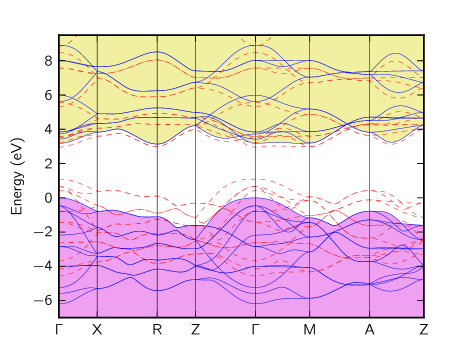
Figure 2: (Color online.) Theoretical band structure of rutile TiO₂ calculated within DFT using the PBE exchange-correlation potential (red dotted lines) and using the GW method (blue solid lines).

Within PBE, the calculated band gap is a direct gap of only $1.86$ eV at the $\Gamma$ point. After applying the GW correction, we found the fundamental gap to be the indirect $\Gamma-\mathrm{R}$ gap of $3.13$ eV although the direct gap at the $\Gamma$ point of $3.18$ eV is very close to the $\Gamma-\mathrm{R}$ gap. A more detailed analysis of the band structure of bulk rutile TiO₂, including the calculation of quasiparticle effective masses, is given in the Supplemental Material.sup

IV.2 Oxygen vacancy

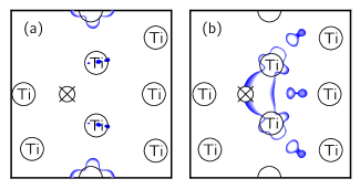
Figure 3: (Color online.) Charge densities of the localized states in the gap found in the HSE calculations with $+1$ charged supercells. Panel (a) shows the ground state, corresponding to a $+2$ charged oxygen vacancy and a polaron. Panel (b) shows the $+1$ charged oxygen vacancy. The isosurfaces show the $10\%$ of the charge densities of the localized states.

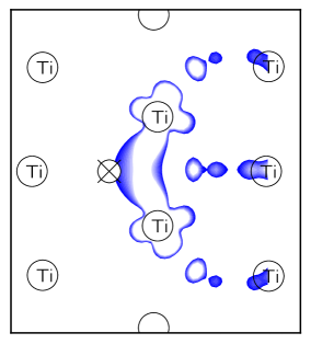
Figure 4: (Color online.) Charge density of the localized defect state of the $+1$ charged oxygen vacancy found in PBE calculation. The isosurface shows the $10\%$ of the charge density. The atomic positions are the same as in Fig. 3 (b).

Qualitatively the important defect state in the gap associated with the oxygen vacancy in rutile TiO₂ can be understood as follows. In bulk rutile, each O atom is surrounded by three neighboring Ti atoms. When one O atom is removed, the three Ti dangling bonds (mostly having $d$ character) form a low-energy state of $a_{1}$ symmetry.Janotti et al. (2010) In the neutral charge state of the oxygen vacancy ($V_{\mathrm{O}}^{0}$), the defect state $a_{1}$ is doubly occupied. In the $+1$ charge state ($V_{\mathrm{O}}^{+}$), the $a_{1}$ is singly occupied. In both cases the occupied $a_{1}$ state bonds the neighboring Ti atoms and keeps them from moving away from the vacancy. In the $+2$ charge state ($V_{\mathrm{O}}^{2+}$), the $a_{1}$ state is unoccupied, which results in a much larger displacements of the Ti atoms outward from the vacancy site.

It is worth noting that if one simply relaxes the $0$ or $+1$ charged systems within PBE, one may find a ground state which does not necessarily correspond to the electrons bound to the vacancy site. Recently, first-principles calculationsDeák et al. (2011, 2012); Janotti et al. (2013) have shown that polarons may form in TiO₂. In addition, experimental evidence of intrinsic polarons in rutile has been seen in electron paramagnetic resonance measurements.Yang et al. (2013) Indeed, in our calculations we find that a naïve relaxation of the $+1$ charged system leads to a ground state with an electron away from the vacancy site. We find a localized state with its eigenvalue in the gap, but the charge density corresponding to this state is not localized at the vacancy site but is localized at the next-nearest neighbor Ti atom. While in principle a polaron can be formed anywhere in the supercell, its localization on the next-nearest Ti atom can be attributed to the finite size of the supercell used in our calculations. Figure 3 (a) shows the calculated charge density of the state in the gap for such a polaron ground state. However, for the purpose of calculation of charge transition levels, this particular state is not appropriate. In order to stabilize the $+1$ vacancy state of interest (i.e., the electron bound to the vacancy site), we used the following procedure. First, we performed a spin-unpolarized relaxation of the neutral vacancy. This resulted in a state with two electrons bound to the vacancy site. Second, we relaxed the $+1$ charged system starting from the atomic configuration found in the first step. This procedure ensured that the defect state remained bound to the vacancy site. Figure 3 (b) shows the charge density of the obtained $+1$ vacancy defect state. We emphasize again that the state thus found is not a ground state (i.e., lowest total energy) in our calculations but rather a local minimum. We found that it is above the ground state (we call it a polaron ground state) by $1.2$ eV.

For the purpose of doing the GW calculation, we used a PBE mean field solution from a structure determined with HSE. This was done because GW calculation requires a large number of empty bands and the computational cost of using HSE as the mean field becomes prohibitive. This is a reasonable procedure because GW is a perturbative correction and does not depend sensitively on the starting mean field. Because our GW calculation is a G₀W₀ calculation, we ensured that the resulting PBE defect wavefunction is similar to the one obtained from HSE. Figure 4 shows the charge density from the defect wavefunction obtained within PBE. Comparing this figure to the Fig. 3 (b), we can see that the defect state charge densities obtained using PBE and HSE for the same structure are similar.

In order to calculate the charge transition levels, we started from $+1$ charged oxygen vacancy. Figure 5 schematically illustrates the paths in formation energy vs generalized coordinate space that we took. It has been shown that all paths in this space give the same value of charge transition levels to within $\pm 0.1$ eV provided that electrostatic corrections are taken into account.Jain et al. (2011) To reduce the computational cost, we performed GW calculation on the $+1$ charged oxygen vacancy. This allows us to calculate both $\epsilon^{1+/0}$ and $\epsilon^{2+/1+}$ as can be seen from Fig. 5. For $\epsilon^{1+/0}$ we computed the quasiparticle (quasielectron) energy of the lowest unoccupied localized state (which in our case turned out to be slightly above the CBM). For $\epsilon^{2+/1+}$ we computed the quasiparticle (quasihole) energy of the $+1$ defect state. Both quasiparticle energies were evaluated relative to the valence band maximum $E_{\mathrm{v}}$, since we defined $\epsilon^{q/q-1}$ relative to $E_{\mathrm{v}}$ in Sec. II.1.

Table 2 shows the results of our computed quasiparticle and relaxation energies as well as the corresponding charge transition levels. From the Table it is clear that the oxygen vacancies are negative $U$ defects, where $U$ is the defect charging energy. Also from the Table, one can see that electrostatic corrections are not negligible and have to be included into the calculation.

Further, one can calculate the absolute formation energies as a function of Fermi energy. For a given chemical potential of oxygen, one needs to know the formation energy of the neutral vacancy, which can be calculated within DFT, since for $q=0$ the absolute values of Kohn-Sham levels do not enter in the definition of formation energy.Jain et al. (2011) Note also that formation energy of the neutral vacancy does not depend on the value of Fermi level $E_{\mathrm{F}}$. Then using the definition of charge transition levels, one can obtain the formation energy for all the charge states for a given chemical potential of oxygen. Namely, for a $+1$ oxygen vacancy $V_{\mathrm{O}}^{+}$ one can write

$$E^{\mathrm{f}}_{1+}(E_{\mathrm{F}})=E^{\mathrm{f}}_{0}-\epsilon^{1+/0}+E_{\mathrm{F}},$$ (6)

while a corresponding relation for $V_{\mathrm{O}}^{2+}$ is

$$E^{\mathrm{f}}_{2+}(E_{\mathrm{F}})=E^{\mathrm{f}}_{0}-\epsilon^{1+/0}-\epsilon^{2+/1+}+2E_{\mathrm{F}}.$$ (7)

It is worth noting that calculating formation energies of the charged defects in this manner does not involve the value of the valence band maximum within mean field. This ensures that the energy scale for the electrons is set only by the GW calculation and not by DFT calculations.

Figure 6 shows our results for formation energy of various charges states of the oxygen vacancy plotted as a function of Fermi energy $E_{\mathrm{F}}$ in the oxygen-rich [Fig. 6 (a)] and oxygen-poor [Fig. 6 (b)] growth conditions. For oxygen-rich growth conditions, the oxygen chemical potential is $\mu_{\mathrm{O}}=0$. In the titanium-rich (oxygen-poor) limit, $\mu_{\mathrm{O}}$ is determined by the formation of Ti₂O₃, which implies the condition $2\mu_{\mathrm{Ti}}+3\mu_{\mathrm{O}}=\Delta{H}_{\mathrm{f}}(\mathrm{Ti}_{2}\mathrm{O}_{3})$. Here $\Delta{H}_{\mathrm{f}}(\mathrm{Ti}_{2}\mathrm{O}_{3})$ is the formation enthalpy of Ti₂O₃, which we found to be $-15.33$ eV (per formula unit). On the other hand, stability condition for the TiO₂ requires $\mu_{\mathrm{Ti}}+2\mu_{\mathrm{O}}=\Delta{H}_{\mathrm{f}}(\mathrm{TiO}_{2})$, where formation enthalpy $\Delta{H}_{\mathrm{f}}(\mathrm{TiO}_{2})=-9.66$ eV (per formula unit). From these two conditions we find the oxygen chemical potential to be $\mu_{\mathrm{O}}=-3.99$ eV in the titanium-rich limit.

As can be seen from Fig. 6, the most stable defects in the wide range of possible values for Fermi energy are $+2$ charged oxygen vacancies. This finding is in qualitative agreement with the previous HSE study by Janotti et al. [see Fig. 5 of Ref. Janotti et al., 2010]. Similar to that work, we also find that the transition from the $+2$ to neutral state occurs at a higher value of $E_{\mathrm{F}}$ than the transition from the neutral to $+1$ state (a feature of the negative $U$ defect). Quantitatively, however, our values for charge transition levels are smaller then what was found in Ref. Janotti et al., 2010 by $\sim 0.5$ eV. To be more precise, charge transition levels in that work were found to be at or above the conduction band minimum and, as a result, the $V_{\mathrm{O}}^{+2}$ was found to be the only stable oxygen vacancy for all values of $E_{\mathrm{F}}$. In our case, we find that for $E_{\mathrm{F}}>2.8$ eV the neutral vacancy can become more stable.

We emphasize that the study of formation energies and relative stability of charged oxygen vacancies in rutile TiO₂ cannot be done at the PBE level since in this case the defect levels are not found in the bulk band gap. Therefore, it is crucial to use more advanced methods, such as, e.g., the one described above.

Table 2: Contributions to the charge transition levels coming from the quasiparticle energy $E_{\mathrm{QP}}$, relaxation energy $E_{\mathrm{relax}}$, and electrostatic correction $\Delta{E}^{\mathrm{e.s.}}_{\mathrm{QP}}$ (all values are given in eV).

	$\epsilon^{2+/1+}$	$\epsilon^{1+/0}$
$E_{\mathrm{QP}}$	$-$2.58	$-$3.24
$E_{\mathrm{relax}}$	$-$0.86	$-$0.29
$\Delta{E}^{\mathrm{e.s.}}_{\mathrm{QP}}$	$-$0.44	$-$0.44
$\epsilon^{q/q-1}$	$-$3.00	$-$2.51

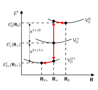
Figure 5: Schematic illustration of the calculation of the charge transition levels $\epsilon^{2+/1+}$ and $\epsilon^{1+/0}$ within the DFT+GW formalism. Arrows indicate the actual paths used in our calculations.

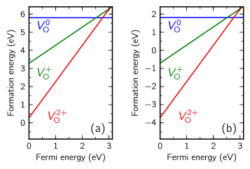
Figure 6: Calculated formation energies of oxygen vacancies in rutile TiO₂ plotted as functions of Fermi level $E_{\mathrm{F}}$ in the (a) oxygen-rich and (b) titanium-rich growth conditions.

V Summary

In summary, we investigated the oxygen vacancies in rutile TiO₂ in three charge states from first principles using the DFT+GW approach. The oxygen vacancies were emulated in a 71 atom supercells. The structural relaxations around the defects were performed using the hybrid functional (HSE) method and charge transition levels and defect formation energies were calculated within the DFT+GW formalism. According to our calculations, in a wide range of values for Fermi energy, $0<E_{\mathrm{F}}<2.8$ eV, the $+2$ charge state of the vacancy is the most stable, while for Fermi energies above $2.8$ eV the neutral vacancy is stabilized. This result also means that oxygen vacancy is found to be a negative $U$ defect.

VI Acknowledgments

This work was supported by National Science Foundation Grant No. DMR10-1006184 (ground-state and structural studies, electrostatic correction analyses, and effective mass calculations) and the Theory Program at the Lawrence Berkeley National Laboratory (LBNL) funded by the Department of Energy (DOE), Office of Basic Energy Sciences, under Contract No. DE-AC02-05CH11231 (quasiparticle calculations and studies of charge transition levels). Algorithm developments for large-scale GW simulations were supported through the Scientific Discovery through Advanced Computing (SciDAC) Program on Excited State Phenomena in Energy Materials funded by DOE, Office of Basic Energy Sciences and of Advanced Scientific Computing Research, under Contract No. DE-AC02-05CH11231 at LBNL. SGL acknowledges support of a Simons Foundation Fellowship in Theoretical Physics. Computational resources have been provided by DOE at Lawrence Berkeley National Laboratory’s NERSC facility and by National Institute for Computational Sciences.

We would like to thank A. Janotti for helpful discussions.

Supplemental Material to “First-principles DFT+GW study of oxygen vacancies in rutile TiO₂”

VII Introduction

In this Supllemental Material we provide the details of calculation of the band structure and quasiparticle effective masses of rutile TiO₂ from first principles within the GW formalism. For quasiparticle eigenvalues, we use a G₀W₀ method based on the Hybertsen-Louie generalized plasmon pole model. Within this model, the convergence of the self-energy is assured by including a sufficient number of conduction bands in the calculation. To further verify the accuracy of the calculations, we perform an additional full-frequency G₀W₀ calculation of the direct band gap at the $\Gamma$ point. We found the fundamental band gap in rutile to be an indirect $\Gamma-\mathrm{R}$ gap of $3.13$ eV. The quasiparticle effective masses are computed for the quasielectrons of the lowest conduction band and quasiholes of the highest valence band using Wannier interpolation technique.

The precise knowledge of the electronic band structure of rutile TiO₂ is crucial for understanding its optical properties. Despite enormous research efforts, both theoretical and experimental, controversies still remain in the evaluation of such basic quantities as quasiparticle band gaps for this material.

Early on rutile was found to have an optical band gap of $3.05$ eV from optical absorption and photoconductivity measurements. app_cronemeyer_51 ; app_cronemeyer_52 ; app_cronemeyer_59 Later measurementsapp_arntz_66 ; app_vos_74 ; app_pascual_77 ; app_pascual_78 ; app_amtout_95 resolved the fine structure of the absorption edge in rutile showing that the first peak in the absorption spectrum appears at $3.031$ eV. On the other hand, photoemission and inverse photoemission experiments have shown that the electronic band gap, defined as the difference between the conduction-band minimum (CBM) and valence-band maximum (VBM), is higher than the optical gap. The reported values for the electronic band gap vary in the range $3.3-4.0$ eVapp_hardman_94 ; app_tezuka_94 ; app_rangan_10 with one of the most accurate values reported recently being $3.6\pm 0.2$ eV.app_rangan_10 The optical properties of anatase and brookite are less studied compared to rutile. The reported values for the optical absorption gaps for anatase and brookite are $\sim 3.4-3.8$ eVapp_tang_95 ; app_wang_02 and $\sim 3.3$ eV, respectively. The electronic band gaps have to be larger than the corresponding optical gaps because of exciton formation. However, to the best of our knowledge, they have not yet been directly measured in these phases.

As for theory, numerous first-principles calculations have been done in the past years. An extensive comparison of values of band gaps for rutile and anatase obtained with different theoretical methods can be found in Ref. app_chiodo_10, . Typically, mean-field calculations based on density-functional theory (DFT) underestimate the band gap substantially. This is a well known problem, which takes its roots from the fact that the Kohn-Sham eigenvalues do not represent actual quasiparticle energies. One of the most successful approaches to mitigate this problem is based on the many-body perturbation theory, employing the so-called GW method. app_hybertsen_86 However, the reported values for band gaps in TiO₂ obtained with the help of GW method still vary significantly. For example, in the case of rutile the values were reported from $2.9$ eV to $4.8$ eV.app_chiodo_10 ; app_patrick_12 ; app_kang_10 There could be several reasons for this broad range of values. On one hand, the GW method itself has many flavors with different level of approximation. It is a subject of many debates regarding to which flavor is appropriate. On the other hand, a typical GW calculation is much more computationally demanding than the corresponding mean-field calculation. It requires a more careful convergence with respect to a larger set of parameters. A fully converged GW calculation is a challenging task but necessary for accurate results. In particular, it has been shown recently that wurtzite ZnO requires several thousands of empty bands to converge the GW band gap calculation.app_shih_10 ; app_friedrich_11 Here, we revisit the problem of the band gap in rutile TiO₂. We perform a GW calculation of the band structure, making sure that convergence with respect to number of bands has been achieved. Based on the band structure data, we also perform calculations of the first effective masses of quasiparticles for specific extremal points of the highest valence and lowest conduction bands.

The rest of the Supplemental Material is organized as follows. Section VIII describes computational details of our DFT and GW calculations. Results are discussed in Sec. IX followed by a summary in Sec. X.

VIII Computational details

In this work, mean-field calculations are carried out using a plane-wave ab initio pseudopotential approach to DFT as implemented within the Quantum ESPRESSO code package.app_QE_09 We used generalized-gradient approximation (GGA) with the Perdew-Burke-Ernzerhof (PBE) parameterizationapp_perdew_96 of the exchange-correlation energy functional. Troullier-Martins norm-conserving pseudopotentialsapp_troullier-prb91 were generated with Ti $3s$ and $3p$ states treated as valence orbitals. The titanium pseudopotential was generated in the Ti⁴⁺ configuration, and the cut-off radii for the $3s$, $3p$, and $3d$ states were chosen to be $0.9$, $0.9$, and $1.0$ a.u., respectively.

The plane-wave basis was determined by an energy cutoff of 200 Ry. The Brillouin zone was sampled by a uniform $4\times 4\times 6$ $k$-point mesh. These parameters were sufficient to obtain a well converged mean-field calculation for the band structure. E.g., the value of the PBE direct band gap at the $\Gamma$ point increases by about $0.01$ eV when the $k$-point mesh is changed to a denser $6\times 6\times 9$ mesh. (The corresponding GW value changes by $0.04$ eV.)

The structural parameters of bulk rutile were determined theoretically. Since the band structure results presented in this Supplemental Material are obtained using the GW method with the starting PBE mean field, for consistency we used PBE structural parameters (see Table I of the main text).

The GW calculations were performed using the BerkeleyGW code package.app_deslippe_12 To ensure convergence with respect to number of empty states in the self-energy calculation, we used $2\,000$ valence plus conduction bands. This number of bands ensures that we include all states within approximately 40 Ry above the Fermi level. In addition, the static remainder methodapp_deslippe_13 was used in order to confirm that convergence has indeed been achieved. As an example, the dependence of the computed highest valence and lowest conduction eigenvalues at the $\Gamma$ point on the number of bands is shown in Fig. S1. One can see from the figure that convergence of the quasiparticle eigenvalues with respect to empty states is rather slow. On the other hand, if one is interested only in the calculation of the differences between the eigenvalues (band gaps, e.g.), the convergence may be achieved faster. E.g., as cen be seen from Fig. S1, the value of the direct band gap computed with 200 bands is only about $0.2$ eV larger then the converged value.

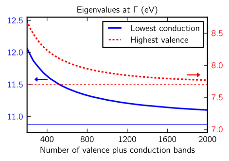
Figure S1: (Color online.) Dependence of the highest valence and lowest conduction quasiparticle eigenvalues at the $\Gamma$ point on the total number of bands used in the self-energy calculation. The horizontal thin lines show the converged values obtained with the static remainder method.

The majority of our GW calculations were performed at the G₀W₀ level employing the generalized plasmon pole (GPP) model and full frequency G₀W₀ method was used at the $\Gamma$ point as an additional check.

For the calculation of the GW quasiparticle band structure the following procedure was used. First, the PBE Kohn-Sham eigenstates and eigenvalues were obtained on a $4\times 4\times 6$ grid of $k$ points. Then the eigenvalues were corrected by employing a G₀W₀ approach within the complex GPP model.app_zhang_89 Finally, Wannier interpolation schemeapp_mostofi_08 ; app_marzari_12 was employed in order to obtain a fine set of eigenvalues along the high-symmetry directions in the Brillouin zone. Within this scheme, the maximally localized Wannier functionsapp_marzari_97 were constructed from the mean-field (PBE) wavefunctions while GW eigenvalues were used at the band structure interpolation step. The accuracy of the Brillouin zone interpolation was checked by doing interpolation starting from $4\times 4\times 6$ and $6\times 6\times 9$ coarse $k$-point grids and comparing the values of effective masses (see next section for details on effective mass calculations). To reduce the computational cost, we did this comparison only at the PBE level. We found that to first two significant digits the values of effective masses did not change, except at the $\Gamma$ point. Therefore, effective masses at this point were calculated separately, without invoking the interpolation procedure.

IX Results

As for the band gap, at the PBE level we found the fundamental gap to be a direct gap of $1.86$ eV at the $\Gamma$ point. At the G₀W₀ level, the gap at $\Gamma$ increased to $3.18$ eV and the fundamental gap became an indirect $\Gamma-\mathrm{R}$ gap of $3.13$ eV, which is still very close to the value of the direct gap at $\Gamma$. While the valence-band maximum clearly occurs at the $\Gamma$ point, the minima of the lowest conduction band at $\Gamma$, $\mathrm{M}$, and $\mathrm{R}$ points are very close. This finding is consistent with previous GW calculations.app_kang_10 ; app_chiodo_10 Kang and Hybertsenapp_kang_10 also found the fundamental gap to be an indirect $\Gamma-\mathrm{R}$ one with a slightly higher value of $3.34$ eV. While Chiodo et al.app_chiodo_10 reported the direct gap at $\Gamma$ to be the lowest one, Fig. $2$ in their paper shows that the lowest GW gap is in fact also $\Gamma-\mathrm{R}$. In any case, the band structure of rutile TiO₂ is found to be rather peculiar, with a direct band gap at $\Gamma$ being very close to the indirect $\Gamma-\mathrm{R}$ and $\Gamma-\mathrm{M}$ gaps.

As discussed in the main text, to study the charged oxygen vacancies in rutile, we had to use hybrid HSE functional for structural relaxations. It is natural to ask then how the value of the GW band gap in rutile depends on the structural parameters of the system. Starting from the HSE parameters shown in Table I of the main text, we performed PBE mean field calculations and applied the GW correction. We found the direct gap at $\Gamma$ in this case to be $3.25$ eV, very close to the value of $3.18$ eV obtained with the PBE structural parameters. Thus, for the purpose of calculation of defect formation energies and charge transition levels, this difference is clearly insignificant, given the number of approximations made (e.g., in the evaluation of electrostatic corrections).

It is also important to check the robustness of GW results with respect to the starting mean field calculation. We performed a one-shot G₀W₀ calculation of the direct gap at $\Gamma$ starting from mean field obtained with local-density approximation (LDA) exchange-correlation functional (using the same HSE structural parameters as above). We found the gap in this case to be $3.28$ eV, very close to the GW value of $3.25$ eV obtained with the PBE reference mean field. For comparison, the LDA gap is $1.77$ eV and the PBE is $1.90$ eV. Thus, the GW correction depends on the reference DFT calculation and adjusts itself in such a way as to give very close final GW values.

In order to assess the accuracy of our GPP G₀W₀ results, we also carried out a full-frequency G₀W₀ calculation. Since this type of calculations is much more computationally demanding than the GPP G₀W₀ calculations, we decided to do a full-frequency integration only at the $\Gamma$ point. The frequency integration was done along the real axisapp_deslippe_12 using regular mesh of frequencies up to $50$ eV with spacing of $0.2$ eV and then using linearly increasing spacing for frequencies up to cutoff of $1\,000$ eV. The direct band gap at $\Gamma$ computed in this fashion was found to be $3.16$ eV, in excellent agreement with our GPP G₀W₀ result.

Using the band-structure data shown in Fig. 2 of the main text,one can determine the effective masses of the quasiparticles at the band extrema. Here we analyze highest valence and lowest conduction bands. Of special interest are the quasiparticles associated with the $\Gamma$, $\mathrm{R}$, and $\mathrm{M}$ points of the Brillouin zone since the lowest conduction band has almost the same energy at these points with conduction band minimum being at $\mathrm{R}$. The point $\mathrm{A}$ is also of interest due to a local maximum of the valence band. Table 1 lists the effective masses calculated at these four points.

Note that tetragonal symmetry of rutile implies that the main axes of the effective mass tensor at $\Gamma$ coincide with the Cartesian axes $k_{x}$, $k_{y}$, and $k_{z}$ [see Fig. 1(b) of the main text], with $k_{x}$ and $k_{y}$ being equivalent. Therefore, the effective mass tensor at this point must be diagonal in $k_{x}-k_{y}$ plane and the effective masses in the columns $\Gamma\rightarrow\mathrm{X}$ and $\Gamma\rightarrow\mathrm{M}$ in Table 1 must be the same. One can see from the Table that apart from small numerical noise this is indeed the case.

The effective mass tensors (both for the highest valence and lowest conduction bands) of rutile at $\Gamma$ is highly anisotropic. Quasi-electrons are less massive by a factor of $\sim 3$ in response to a perturbation along $z$ direction compared to a response perpendicular to $z$ axis. Quasi-holes at $\Gamma$, however, are more massive along $z$ direction. They are also heavier compared to quasi-electrons. Interestingly, compared to other band minima, quasi-electrons at $\Gamma$ are both the heaviest and the lightest depending on the direction of response.

The computed effective masses are in reasonable agreement with previous $\sigma$-GGA and $\sigma$-GGA$+U$ calculations,app_perevalov_11 except for the $\Gamma\rightarrow(\mathrm{X},\mathrm{M})$ electron effective mass, which in our case is an order of magnitude smaller than the $\sigma$-GGA$+U$ value. The experimental values for the electron effective masses are reported in a wide range, from $\sim 0.7$ $m_{e}$app_stamate_03 to $\sim 3$ $m_{e}$,app_pascual_77 ; app_pascual_78 where $m_{e}$ is the electron mass in vacuum. The wide range of reported values may be partially attributed to the polaron effectsapp_pascual_78 in TiO₂ and associated difficulties in extracting the bare effective mass from the polaron effective mass in this case. The polaron effects on the effective masses are not considered in the present work.

Table 1: Calculated effective masses for rutile TiO₂ expressed in units of the electron mass, $m_{e}$. Negative sign indicates holes. Notation $P_{1}\rightarrow{P_{2}}$ specifies that effective mass was computed from the band curvature in the vicinity of point $P_{1}$ in direction towards point $P_{2}$.

PBE	$\Gamma\rightarrow\mathrm{X}$	$\Gamma\rightarrow\mathrm{M}$	$\Gamma\rightarrow\mathrm{Z}$	$\mathrm{R}\rightarrow\mathrm{X}$	$\mathrm{R}\rightarrow\mathrm{Z}$	$\mathrm{A}\rightarrow\mathrm{M}$	$\mathrm{M}\rightarrow\mathrm{A}$
Conduction band	$\phantom{-}1.2$	$\phantom{-}1.2$	$\phantom{-}0.6$	$\phantom{-}1.0$	$\phantom{-}0.6$	$\phantom{-}1.1$	$\phantom{-}0.8$
Valence band	$-3.1$	$-3.1$	$-5.3$	$-3.0$	$-0.5$	$-1.6$	$-1.2$
GW	$\Gamma\rightarrow\mathrm{X}$	$\Gamma\rightarrow\mathrm{M}$	$\Gamma\rightarrow\mathrm{Z}$	$\mathrm{R}\rightarrow\mathrm{X}$	$\mathrm{R}\rightarrow\mathrm{Z}$	$\mathrm{A}\rightarrow\mathrm{M}$	$\mathrm{M}\rightarrow\mathrm{A}$
Conduction band	$\phantom{-}1.4$	$\phantom{-}1.5$	$\phantom{-}0.6$	$\phantom{-}1.0$	$\phantom{-}0.7$	$\phantom{-}1.1$	$\phantom{-}0.8$
Valence band	$-2.4$	$-2.4$	$-3.6$	$-3.5$	$-0.6$	$-1.4$	$-1.0$

X Summary

We performed a theoretical study of the basic electronic structure properties, such as the quasiparticle band structure and effective masses, of rutile TiO₂ by means of first-principles calculations based on the GPP G₀W₀ method. Strict convergence criteria required us to use about $2\,000$ conduction bands in the evaluation of the self-energy. The accuracy of the method was cross checked by performing an additional full frequency G₀W₀ calculation. Our band gap results for rutile are in good agreement with previous GW and experimental studies. In particular, we found the fundamental gap to be an indirect $\Gamma-\mathrm{R}$ one. The value of the gap was found to be $3.13$ eV. The quasiparticle eigenvalues were evaluated on a mesh of $k$ points and then interpolated to high symmetry lines in the Brillouin zone allowing us to evaluate the effective masses. The quasiparticle effective masses were computed for certain local extrema of the lowest conduction and highest valence bands. We found the effective masses to be highly anisotropic for both quasielectrons and quasiholes. The quasielectron effective masses vary from $0.6$ $m_{e}$ to $1.5$ $m_{e}$, while the quasiholes are generally heavier and have masses from $0.6$ $m_{e}$ to $3.6$ $m_{e}$ depending on direction.

References

- Grant (1959) F. A. Grant, Rev. Mod. Phys. 31, 646 (1959).
- Diebold (2003) U. Diebold, Surf. Sci. Reports 48, 53 (2003).
- Augustynski (1993) J. Augustynski, Electrochimica Acta 38, 43 (1993).
- Linsebigler et al. (1995) A. L. Linsebigler, G. Lu, and J. T. Yates, Jr., Chem. Rev. 95, 735 (1995).
- O’Regan and Grätzel (1991) B. O’Regan and M. Grätzel, Nature (London) 353, 737 (1991).
- Yang et al. (2008) J. J. Yang, M. D. Pickett, X. Li, D. A. A. Ohlberg, D. R. Stewart, and R. S. Williams, Nature Nanotechnology 3, 429 (2008).
- Kim et al. (2008) S. K. Kim, G.-J. Choi, S. Y. Lee, M. Seo, S. W. Lee, J. H. Han, H.-S. Ahn, S. Han, and C. S. Hwang, Adv. Mater. 20, 1429 (2008).
- Wilk et al. (2001) G. D. Wilk, R. M. Wallace, and J. M. Anthony, J. Appl. Phys. 89, 5243 (2001).
- Fujishima and Honda (1972) A. Fujishima and K. Honda, Nature (London) 238, 37 (1972).
- Abrahams and Bernstein (1971) S. C. Abrahams and J. L. Bernstein, J. Chem. Phys. 55, 3206 (1971).
- Cronemeyer (1959) D. C. Cronemeyer, Phys. Rev. 113, 1222 (1959).
- Amtout and Leonelli (1995) A. Amtout and R. Leonelli, Phys. Rev. B 51, 6842 (1995).
- Tezuka et al. (1994) Y. Tezuka, S. Shin, T. Ishii, T. Ejima, S. Suzuki, and S. Sato, J. Phys. Soc. Jpn. 63, 347 (1994).
- Hardman et al. (1994) P. J. Hardman, G. N. Raikar, C. A. Muryn, G. van der Laan, P. L. Wincott, G. Thornton, D. W. Bullett, and P. A. D. M. A. Dale, Phys. Rev. B 49, 7170 (1994).
- Rangan et al. (2010) S. Rangan, S. Katalinic, R. Thorpe, R. A. Bartynski, J. Rochford, and E. Galoppini, J. Phys. Chem. C 114, 1139 (2010).
- Chiodo et al. (2010) L. Chiodo, J. M. García-Lastra, A. Iacomino, S. Ossicini, J. Zhao, H. Petek, and A. Rubio, Phys. Rev. B 82, 045207 (2010).
- Hedström et al. (2006) M. Hedström, A. Schindlmayr, G. Schwarz, and M. Scheffler, Phys. Rev. Lett. 97, 226401 (2006).
- Rinke et al. (2009) P. Rinke, A. Janotti, M. Scheffler, and C. G. Van de Walle, Phys. Rev. Lett. 102, 026402 (2009).
- Jain et al. (2011) M. Jain, J. R. Chelikowsky, and S. G. Louie, Phys. Rev. Lett. 107, 216803 (2011).
- Iddir et al. (2007) H. Iddir, S. Öğüt, P. Zapol, and N. D. Browning, Phys. Rev. B 75, 073203 (2007).
- Peng et al. (2013) H. Peng, D. O. Scanlon, V. Stevanovic, J. Vidal, G. W. Watson, and S. Lany, Phys. Rev. B 88, 115201 (2013).
- Hybertsen and Louie (1986) M. S. Hybertsen and S. G. Louie, Phys. Rev. B 34, 5390 (1986).
- Cohen et al. (1975) M. L. Cohen, M. Schlüter, J. R. Chelikowsky, and S. G. Louie, Phys. Rev. B 12, 5575 (1975).
- Freysoldt et al. (2009) C. Freysoldt, J. Neugebauer, and C. G. Van de Walle, Phys. Rev. Lett. 102, 016402 (2009).
- Chen and Pasquarello (2013) W. Chen and A. Pasquarello, Phys. Rev. B 88, 115104 (2013).
- Janotti et al. (2010) A. Janotti, J. B. Varley, P. Rinke, N. Umezawa, G. Kresse, and C. G. Van de Walle, Phys. Rev. B 81, 085212 (2010).
- Heyd et al. (2003) J. Heyd, G. E. Scuseria, and M. Ernzerhof, J. Chem. Phys. 118, 8207 (2003).
- Heyd et al. (2006) J. Heyd, G. E. Scuseria, and M. Ernzerhof, J. Chem. Phys. 124, 219906(E) (2006).
- Perdew et al. (1996) J. P. Perdew, K. Burke, and M. Ernzerhof, Phys. Rev. Lett. 77, 3865 (1996).
- Blöchl (1994) P. E. Blöchl, Phys. Rev. B 50, 17953 (1994).
- Kresse and Joubert (1999) G. Kresse and D. Joubert, Phys. Rev. B 59, 1758 (1999).
- Kresse and Furthmüller (1996a) G. Kresse and J. Furthmüller, Phys. Rev. B 54, 11169 (1996a).
- Kresse and Furthmüller (1996b) G. Kresse and J. Furthmüller, Comput. Mater. Sci. 6, 15 (1996b).
- Giannozzi et al. (2009) P. Giannozzi, S. Baroni, N. Bonini, M. Calandra, R. Car, C. Cavazzoni, D. Ceresoli, G. L. Chiarotti, M. Cococcioni, I. Dabo, A. Dal Corso, S. de Gironcoli, S. Fabris, G. Fratesi, R. Gebauer, U. Gerstmann, C. Gougoussis, A. Kokalj, M. Lazzeri, L. Martin-Samos, N. Marzari, F. Mauri, R. Mazzarello, S. Paolini, A. Pasquarello, L. Paulatto, C. Sbraccia, S. Scandolo, G. Sclauzero, A. P. Seitsonen, A. Smogunov, P. Umari, and R. M. Wentzcovitch, J. Phys.: Condens. Matter 21, 395502 (19pp) (2009).
- Troullier and Martins (1991) N. Troullier and J. L. Martins, Phys. Rev. B 43, 1993 (1991).
- Deslippe et al. (2012) J. Deslippe, G. Samsonidze, D. A. Strubbe, M. Jain, M. L. Cohen, and S. G. Louie, Comput. Phys. Commun. 183, 1269 (2012).
- Zhang et al. (1989) S. B. Zhang, D. Tománek, M. L. Cohen, S. G. Louie, and M. S. Hybertsen, Phys. Rev. B 40, 3162 (1989).
- Deslippe et al. (2013) J. Deslippe, G. Samsonidze, M. Jain, M. L. Cohen, and S. G. Louie, Phys. Rev. B 87, 165124 (2013).
- (39) See Supplemental Material at [] for further details on the calculations of the electronic band structure and quasiparticle effective masses of bulk rutile TiO2.
- Deák et al. (2011) P. Deák, B. Aradi, and T. Frauenheim, Phys. Rev. B 83, 155207 (2011).
- Deák et al. (2012) P. Deák, B. Aradi, and T. Frauenheim, Phys. Rev. B 86, 195206 (2012).
- Janotti et al. (2013) A. Janotti, C. Franchini, J. B. Varley, G. Kresse, and C. G. Van de Walle, Phys. Status Solidi RRL 7, 199 (2013).
- Yang et al. (2013) S. Yang, A. T. Brant, N. C. Giles, and L. E. Halliburton, Phys. Rev. B 87, 125201 (2013).

References

- (1) D. C. Cronemeyer and M. A. Gilleo, Phys. Rev. 82, 975 (1951)
- (2) D. C. Cronemeyer, Phys. Rev. 87, 876 (1952)
- (3) D. C. Cronemeyer, Phys. Rev. 113, 1222 (1959)
- (4) F. Arntz and Y. Yacoby, Phys. Rev. Lett. 17, 857 (1966)
- (5) K. Vos and H. J. Krusemeyer, Solid State Commun. 15, 949 (1974)
- (6) J. Pascual, J. Camassel, and H. Mathieu, Phys. Rev. Lett. 39, 1490 (1977)
- (7) J. Pascual, J. Camassel, and H. Mathieu, Phys. Rev. B 18, 5606 (1978)
- (8) A. Amtout and R. Leonelli, Phys. Rev. B 51, 6842 (1995)
- (9) P. J. Hardman, G. N. Raikar, C. A. Muryn, G. van der Laan, P. L. Wincott, G. Thornton, D. W. Bullett, and P. A. D. M. A. Dale, Phys. Rev. B 49, 7170 (Mar 1994)
- (10) Y. Tezuka, S. Shin, T. Ishii, T. Ejima, S. Suzuki, and S. Sato, J. Phys. Soc. Jpn. 63, 347 (1994)
- (11) S. Rangan, S. Katalinic, R. Thorpe, R. A. Bartynski, J. Rochford, and E. Galoppini, J. Phys. Chem. C 114, 1139 (2010)
- (12) H. Tang, F. Lévy, H. Berger, and P. E. Schmid, Phys. Rev. B 52, 7771 (1995)
- (13) Z. Wang, U. Helmersson, and P.-O. Käll, Thin Solid Films 405, 50 (2002)
- (14) L. Chiodo, J. M. García-Lastra, A. Iacomino, S. Ossicini, J. Zhao, H. Petek, and A. Rubio, Phys. Rev. B 82, 045207 (2010)
- (15) M. S. Hybertsen and S. G. Louie, Phys. Rev. B 34, 5390 (1986)
- (16) C. E. Patrick and F. Giustino, J. Phys.: Condens. Matter 24, 202201 (2012)
- (17) W. Kang and M. S. Hybertsen, Phys. Rev. B 82, 085203 (2010)
- (18) B.-C. Shih, Y. Xue, P. Zhang, M. L. Cohen, and S. G. Louie, Phys. Rev. Lett. 105, 146401 (2010)
- (19) C. Friedrich, M. C. Müller, and S. Blügel, Phys. Rev. B 83, 081101 (2011)
- (20) P. Giannozzi, S. Baroni, N. Bonini, M. Calandra, R. Car, C. Cavazzoni, D. Ceresoli, G. L. Chiarotti, M. Cococcioni, I. Dabo, A. Dal Corso, S. de Gironcoli, S. Fabris, G. Fratesi, R. Gebauer, U. Gerstmann, C. Gougoussis, A. Kokalj, M. Lazzeri, L. Martin-Samos, N. Marzari, F. Mauri, R. Mazzarello, S. Paolini, A. Pasquarello, L. Paulatto, C. Sbraccia, S. Scandolo, G. Sclauzero, A. P. Seitsonen, A. Smogunov, P. Umari, and R. M. Wentzcovitch, J. Phys.: Condens. Matter 21, 395502 (19pp) (2009), http://www.quantum-espresso.org
- (21) J. P. Perdew, K. Burke, and M. Ernzerhof, Phys. Rev. Lett. 77, 3865 (1996)
- (22) N. Troullier and J. L. Martins, Phys. Rev. B 43, 1993 (1991)
- (23) J. Deslippe, G. Samsonidze, D. A. Strubbe, M. Jain, M. L. Cohen, and S. G. Louie, Comput. Phys. Commun. 183, 1269 (2012)
- (24) J. Deslippe, G. Samsonidze, M. Jain, M. L. Cohen, and S. G. Louie, Phys. Rev. B 87, 165124 (2013)
- (25) S. B. Zhang, D. Tománek, M. L. Cohen, S. G. Louie, and M. S. Hybertsen, Phys. Rev. B 40, 3162 (Aug 1989)
- (26) A. A. Mostofi, J. R. Yates, Y.-S. Lee, I. Souza, D. Vanderbilt, and N. Marzari, Comput. Phys. Commun. 178, 685 (2008)
- (27) N. Marzari, A. A. Mostofi, J. R. Yates, I. Souza, and D. Vanderbilt, Rev. Mod. Phys. 84, 1419 (Oct 2012)
- (28) N. Marzari and D. Vanderbilt, Phys. Rev. B 56, 12847 (1997)
- (29) T. V. Perevalov and V. A. Gritsenko, Journal of Experimental and Theoretical Physics 112, 310 (2011)
- (30) M. D. Stamate, Appl. Surf. Sci. 205, 353 (2003)