Charged Rényi entropies and holographic superconductors

Abstract

Charged Rényi entropies were recently introduced as a measure of entanglement between different charge sectors of a theory. We investigate the phase structure of charged Rényi entropies for CFTs with a light, charged scalar operator. The charged Rényi entropies are calculated holographically via areas of charged hyperbolic black holes. These black holes can become unstable to the formation of scalar hair at sufficiently low temperature; this is the holographic superconducting instability in hyperbolic space. This implies that the Rényi entropies can be non-analytic in the Rényi parameter $n$. We find the onset of this instability as a function of the charge and dimension of the scalar operator. We also comment on the relation between the phase structure of these entropies and the phase structure of a holographic superconductor in flat space.

1 Introduction

The low energy states of a quantum field theory typically exhibit a high degree of spatial entanglement. To characterize this entanglement precisely, consider a quantum field theory in state $\rho$, with space divided into two parts $A\cup B$. The Rényi entropies $S_{n}$ are the moments of the reduced density matrix $\rho_{\textrm{\tiny A}}={\mathop{\mathrm{Tr}}}_{B}\rho$ for subsystem $A$

$$S_{n}={1\over 1-n}\log{\mathop{\mathrm{Tr}}}[\rho_{\textrm{\tiny A}}^{n}].$$ (1)

The entanglement entropy $S_{EE}$ is $S_{EE}=\lim_{n\to 1}S_{n}=-{\mathop{\mathrm{Tr}}}\rho_{\textrm{\tiny A}}\log\rho_{\textrm{\tiny A}}$. These entropies encode the amount of information stored in correlations between $A$ and $B$, rather than in $A$ or $B$ separately. Entanglement entropies have played an important role in condensed matter physics wenx ; cardy0 , quantum gravity Kabat:1994vj ; rt0 ; mvr , and quantum information Horodecki:2009zz .

In many cases we are interested in theories with a conserved charge $Q$ associated with a global symmetry, such as particle number. When $Q$ is the integral of a local charge density one can ask how the entanglement depends on the distribution of charge between $A$ and $B$. Very naively, one might expect that the entanglement between $A$ and $B$ should increase as charge is distributed more and more unequally between $A$ and $B$. This is because one way of moving charge (say, particle number) into $A$ from $B$ is to create a particle-antiparticle pair, placing the particle in region $A$ and the anti-particle in region $B$; particle-antiparticle pairs created from the vacuum are naturally entangled, so this process should increase the entanglement entropy. Of course, whether this naive expectation is true will depend on the details of the state and the theory.

To address this question we will follow Belin:2013uta and define the charged Rényi entropy:

$$S_{n}(\mu)={1\over 1-n}\log\mathop{\mathrm{Tr}}\left[\,\rho_{\textrm{\tiny A}}\,\frac{e^{\mu\,Q_{\textrm{\tiny A}}}}{{\cal N}_{\textrm{\tiny A}}(\mu)}\right]^{n}\,.$$ (2)

The parameter $\mu$ is known as an entanglement chemical potential, and $Q_{\textrm{\tiny A}}$ measures the amount of charge in subsystem $A$; it is the integral over A of the local charge density. ${\cal N}_{\textrm{\tiny A}}(\mu)\equiv\mathop{\mathrm{Tr}}[\rho_{A}e^{\mu\,Q_{\textrm{\tiny A}}}]$ is a normalization factor. Applications of charged Rényi entropies include the supersymmetric Rényi entropies Nishioka:2013haa and the characterization of symmetry protected topological phases ourSPT .

We emphasize that $\mu$ is not the physical chemical potential of the system, but rather is a formal parameter used to weight the entanglement in different charge sectors. Nevertheless, just as thermodynamic entropies can undergo phase transitions as temperatures and potentials are varied, the entanglement entropies $S_{n}(\mu)$ can undergo phase transitions as the Rényi parameter $n$ and the entanglement chemical potential $\mu$ are varied. These phase transitions reflect essentially non-analytic features of the spatial entanglement structure of quantum field theory ground states.

Rényi phase transitions were investigated in Belin:2013dva in the case $\mu=0$. The authors considered large $N$ conformal field theories which are dual to semi-classical Einstein gravity in Anti-de Sitter space plus matter. When the entangling surface $\partial A$ is a sphere, $S_{n}$ is related to the entropy of a black hole with hyperbolic event horizon. They showed that $S_{n}$ is non-analytic in $n$ if the dimension $\Delta$ of the lightest scalar operator ${\cal O}$ in the theory is sufficiently small. In particular, $\partial_{n}^{2}S_{n}$ becomes discontinuous at some $n=n_{c}$, with $1<n_{c}<\infty$, if

$$\frac{d-2}{2}<\Delta<\frac{d+\sqrt{d}}{2}\,.$$ (3)

Here $d$ is the space-time dimensionality of the CFT and the first inequality is the unitarity bound. The point is that the field $\phi$ dual to ${\cal O}$ will become unstable if the black hole temperature is sufficiently small. When $n<n_{c}$, $S_{n}$ is computed by the entropy of a Einstein gravity black hole. But when $n>n_{c}$ the Einstein black hole becomes unstable and the scalar operator gets a non-zero expectation value near the horizon. In this phase the entangling surface hosts a localized ”impurity” operator with non-vanishing expectation value. We emphasize that this argument relies crucially on the fact that we are studying theories at large $N$.

Similar results have been found in purely QFT analysis sachdevON ; Steph-Rnyi-tran . These authors consider the renormalization group flow of the coupling constants associated to impurity operators localized on the entangling surface. At a certain value of $n$, the beta functions for these couplings change sign and the system undergoes a phase transition. For example, in sachdevON it was argued that the Rényi entropies of the $O(N)$ model are non-analytic at $n=7/4$.

One consequence of this is that the replica trick – where one computes $S_{EE}$ by computing $S_{n}$ at integer values of $n$ and analytically continuing to $n\to 1$ – must be treated with care. However, we emphasize that in the above analysis $n_{c}$ was shown to be always greater than 1, and approaches $1$ only as the dimension $\Delta$ approaches the unitarity bound (at which point the operator should decouple from the theory). Thus the Rényi entropies are still analytic in a finite neighbourhood of $n=1$. So this result does not invalidate the derivation of the Ryu-Takayanagi formula by Maldacena and Lewkowycz Lewkowycz:2013nqa , which relied only on analyticity near $n=1$. Further relations between the Ryu-Takayanagi formula and Rényi entropies at $n\neq 1$ were discussed in Headrick:2010zt ; Fursaev:2012mp ; Pastras:2014oka .

In this paper we investigate the phase transitions of charged Rényi entropies. We consider large $N$ CFTs with global conserved charges that are holographically dual to Einstein-Maxwell-Scalar theory in AdS. We will be interested in the charged Rényi entropies of the ground state for spherical entangling surfaces; these Rényi entropies can be computed by studying the CFT in hyperbolic space at finite temperature and charge density casini9 ; Belin:2013uta . In the bulk, the dual states are charged AdS black holes with hyperbolic event horizons renyi ; Belin:2013uta .

We will therefore study the phase structure of charged, hyperbolic black holes in AdS. In particular, we will consider instabilities where a charged scalar field – dual to a CFT operator with global charge $q$ – condenses near the horizon. In this paper, we will find that charged entropies $S_{n}(\mu)$ will be non-analytic as we vary $n$ and $\mu$, provided the conformal dimension of the charged operator lies between

$$\frac{d-2}{2}<\Delta_{c}(q)<\frac{1}{2}\left(d+\sqrt{d+\frac{8(d-2)q^{2}\mu^{2}}{8\pi^{2}R^{2}+(d-2)\mu^{2}}}\right)\,.$$ (4)

The setup is very similar to that used in the study of holographic superconductors Hartnoll:2008kx ; Gubser:2008px , the only difference being that space is hyperbolic. The qualitative features of these instabilities are similar to those in flat space. In particular, the high temperature and large chemical potential behaviour is identical to that of the flat-space holographic superconductor; in these limits the curvature of the hyperbolic spatial slice is irrelevant. Thus, even though the charged Rényi entropies under consideration probe only properties of the ground state, they contain information about the phase structure of physical thermodynamic quantities at finite temperature. This echoes the results of haldane ; fu , that entanglement entropies of the ground state can be used to study phase transitions of the theory involving higher excited states.

In Section 2, we review the relationship between the reduced density matrix for spherical entangling surfaces and thermal density matrices in hyperbolic space. In section 3 we relate this to black hole entropy using AdS/CFT, and describe the phase transition using both analytic and numerical techniques. We compute the critical Rényi parameter $n_{c}$ numerically using a shooting method. In Section 4, we discuss these results and relate them to the phase structure of the holographic superconductor in certain limits.

2 From entanglement entropy to thermal entropy

In a relativistic theory, an observer undergoing constant acceleration has causal access only to part of the space-time, known as the Rindler wedge, which is separated from the rest of the space-time by an event horizon. This Rindler wedge is the causal development of half-space, and a Rindler observer is in a thermal state due to the Unruh effect. From this one concludes that the reduced density matrix associated with the half-space is just the thermal density matrix on Rindler space Kabat:1994vj . In a conformal theory, this can be generalized to relate the reduced density matrix for a spherical region and the thermal density matrix on a hyperbolic space casini9 ; renyi . We will now review this argument.

Consider a quantum field on a $d$-dimensional flat space in Euclidean signature

$$ds^{2}_{R^{d}} = dt_{E}^{2}+dr^{2}+r^{2}d\Omega_{d-2}^{2}$$ (5)

where $t_{E}$ is the Euclidean time, $d\Omega_{d-2}$ is the volume element of a unit sphere, and $r$ is the radial coordinate. We are interested in the reduced density matrix of the $d-1$ dimensional ball of radius $R$ centered at the origin. To compute this, we use the fact that flat space metric is conformal to $S^{1}\times\mathbb{H}^{d-1}$:

$$ds^{2}_{R^{d}} = \Omega^{-2}ds^{2}_{S^{1}\times\mathbb{H}^{d}}=\Omega^{-2}(d\tau_{E}^{2}+R^{2}(du^{2}+\sinh^{2}ud\Omega^{2}_{d-2}))$$ (6)

where

$$\Omega=\left|1+\cosh\left(u+i{\tau_{E}\over R}\right)\right|.$$ (7)

and the $S^{1}\times\mathbb{H}^{d-1}$ coordinates $(\tau_{E},u)$ are defined by

$$\exp\left[{-\left(u+i{\tau_{E}\over R}\right)}\right]={R-(r+it_{E})\over R+(r+it_{E})}.$$ (8)

This conformal map has two important features. First, the $\tau_{E}=0$ slice of the $S^{1}\times\mathbb{H}^{d-1}$ geometry covers only the interior of the ball $(t_{E}=0,r=R)$; the entangling surface at $(t_{E}=0,r=R)$ has been mapped to the boundary of the hyperbolic space $u\to\infty$. In Lorentzian signature (taking $\tau_{E}=i\tau$), this coordinate patch would cover only the interior of the Causal region associated with the ball $(t=0,r<R)$. Second, from (8) we see that Euclidean time coordinate $\tau_{E}$ is periodic with period $2\pi R$. Putting this together, we see that the reduced density matrix is (up to a unitary transformation which does not enter into the trace)

$$\rho={1\over Z_{1}}e^{-2\pi RH_{E}}$$ (9)

Here $H_{E}=i{\partial\over\partial\tau_{E}}$ is the Hamiltonian which generates translations in $\tau$ and $Z_{1}$ is a normalization factor. Thus the reduced density matrix for a spherical region of radius $R$ is equivalent to the thermal density matrix on a hyperbolic space with radius $R$ and temperature $T_{0}=1/2\pi R$. From this, one can show that the Rényi entropy (1) is

$$S_{n}={1\over n-1}(n\log Z_{1}-\log Z_{n}),$$ (10)

where $Z_{n}$ is the thermal partition function of the hyperbolic space at $T=T_{0}/n$.

In a theory with a global conserved charge $Q$, one can generalize (9) to

$$\rho_{\mu}=\frac{e^{-H_{E}/T_{0}+\mu Q}}{Z(T_{0},\mu)}\,.$$ (11)

where $Z(T,\mu)$ is a partition function evaluated at temperature $T$ and chemical potential $\mu$. The operator $Q$ measures the charge on hyperbolic space $\mathbb{H}^{d-1}$, which – from the conformal transformations above – simply measures the amount of charge in region $A$. So (11) is the generalized reduced density matrix introduced in (2).

Note that $\mu$ can be interpreted as the time component of a background gauge field $B_{\mu}$ which couples to the charge density, via $B_{\tau_{E}}=\mu/2\pi R$

$$\mu=\oint B=\int_{0}^{2\pi R}B_{\tau_{\textrm{\tiny E}}}d\tau_{\textrm{\tiny E}}\,.$$ (12)

Since the $\tau_{E}$ circle shrinks to zero at the entangling surface, this chemical potential introduces a magnetic flux localized at the entangling surface Belin:2013uta . The charged Rényi entropies

$$S_{n}(\mu)={1\over 1-n}\log\frac{Z(T_{0}/n,\mu)}{Z(T_{0},\mu)^{n}}.$$ (13)

measure the entanglement in the (flat space, zero charge density) ground state of a theory, weighted by the charge contained in region A. In fact, using the thermodynamic identity

$$S_{\text{therm}}(T,\mu)=-\left.{\partial F(T,\mu)\over\partial T}\right|_{\mu}={\partial\over\partial T}(T\log Z(T,\mu))\big{|}_{\mu}\,.$$ (14)

this can be written in terms of the standard grand canonical ensemble thermal entropy $S_{therm}(T,\mu)$:

$$S_{n}(\mu)={n\over n-1}{1\over T_{0}}\int_{T_{0}/{n}}^{T_{0}}S_{\text{therm}}(T,\mu)\,dT\,.$$ (15)

Finally, it is important to mention the cut-off dependence of the Rényi entropy. The Rényi entropy, as well as the entanglement entropy, are divergent quantities unless we set a UV cut-off near the entangling surface. On the other hand, the thermal entropy on hyperbolic space is a divergent quantity as the volume of the hyperboloid is infinite; we must set an IR cut-off near the boundary of hyperbolic space. In fact, these divergences are identical: they can be mapped into one another by the conformal transformation (6). We refer the reader to casini9 for more details.

3 Holographic computations

In this section we calculate charged Rényi entropies for large $N$ CFTs which are dual to semi-classical Einstein gravity coupled to matter in AdS space. In this case $S_{therm}(T,\mu)$ is the entropy of a black hole entropy in the bulk with hyperbolic event horizon casini9 ; renyi . The global conserved current of the boundary theory acts as a source for a bulk gauge field. We will also assume the existence of a scalar operator in the boundary theory, with dimension $\Delta$ and charge $q$, which is dual to a charged scalar field in the bulk. We are therefore looking for charged black holes with hyperbolic event horizons in Einstein-Maxwell-Scalar theory. These solutions are dual to the grand canonical ensemble of the boundary CFT on $\mathbb{R}\times\mathbb{H}^{d-1}$. We first describe the Einstein-Maxwell solutions and give the Rényi entropies when there is no scalar condensate. We then look for scalar instabilities for the Einstein-Maxwell black hole at the linearized level. We perform an analytic analysis of the extremal black hole, and show that instabilities do occur in this case. We then solve the Klein-Gordon equation for the scalar in the non-extremal case, using a numerical shooting method starting from the horizon. This allows us to determine the location of the phase transition in $S_{n}(\mu)$ as a function of $\Delta$ and $q$. We focus here on 3-dimensional CFT but a similar phase transition will occur in any dimension $d\geq 3$.

3.1 Neutral black holes and scalar instability

Before discussing the charged Rényi entropies and the related charged hyperbolic black holes, we review a few result concerning uncharged black holes. When the entangling chemical potential vanishes, the dual gravitational solutions are hyperbolic black holes

$$ds^{2}=-f(r)\frac{L^{2}}{R^{2}}\,d\tau^{2}+\frac{dr^{2}}{f(r)}+r^{2}\,d\mathbb{H}_{2}^{2}\,,$$ (16)

where $d\mathbb{H}_{2}^{2}=du^{2}+\sinh^{2}\!u\,d\phi^{2}$ is the metric on $\mathbb{H}_{2}$ with unit curvature and

$$f(r)=\frac{r^{2}}{L^{2}}-1-\frac{M}{r}$$ (17)

In the entanglement entropy limit $n\to 1$, we recover the massless hyperbolic black hole, which is AdS₄ in Rindler coordinates. To compute the Rényi entropies, we integrate over a range of temperatures (15). As $n$ increases, the integral includes lower and lower temperatures.

We now consider a scalar field in the bulk of negative mass-squared, which is dual to an operator of dimension $\Delta<3$ in the boundary CFT. In this case the black hole may become unstable at a certain temperature $T_{c}$ (or equivalently at a certain $n_{c}$) at which the black hole undergoes a second order phase transition. This was shown in Belin:2013dva , although in earlier work the authors of Dias:2010ma noted a similar instability for topological black holes with compact horizon (see also Martinez:2004nb ). This effect can be understood as follows. In the extremal limit these black holes have a $AdS_{2}\times\mathbb{H}_{2}$ near horizon geometry. Scalar fields with masses below the effective Breitenlohner-Freedman bound for the near-horizon $AdS_{2}$ (suitably corrected for the $\mathbb{H}_{2}$ factor) will become unstable at low temperatures. We emphasize that this happens for uncharged black holes; for AdS black holes with flat or spherical horizons, such instabilities occur only at finite chemical potential. When the scalar field is below this bound the black hole becomes unstable and will decay to a black hole solution with scalar hair. The corresponding boundary operator acquires a non-zero expectation value.

This instability implies that $S_{n}$ has a phase transition as a function of $n$. The Rényi entropies are obtained from the thermal entropies by integrating once so $\partial_{n}^{2}S_{n}$ will become discontinuous at some critical Rényi parameter $n_{c}$. In order to determine the precise value of $n_{c}$ at which this transition occurs, it is necessary to study numerically the scalar wave equation in the black hole background. The results of Belin:2013dva (see also sachdevON ; Steph-Rnyi-tran ) show that $n_{c}>1$ as long $\Delta$ is above the unitarity bound. In particular, if we compute the entanglement entropy by taking $n\to 1$ then $S_{n}$ is given by the Einstein black hole with vanishing scalar field. We will see that this is no longer the case for charged Rényi entropies: when $\mu\neq 0$, it is possible for $n_{c}$ to be less than one.

3.2 Charged black hole

The Einstein-Maxwell-Scalar action with a negative cosmological constant is

$$I_{E-M}=\frac{1}{2\ell_{\textrm{\tiny P}}^{2}}\int d^{4}x\,\sqrt{-g}\left(\frac{6}{L^{2}}+\mathcal{R}-\frac{\ell_{*}^{2}}{4}F_{\mu\nu}F^{\mu\nu}-V(|\phi|)-\frac{1}{2}|\nabla\phi-iqA\phi|^{2}\right)\,.$$ (18)

We will take the potential to be a mass term $V(|\phi|)=\frac{1}{2}m^{2}|\phi|^{2}$ which, together with boundary conditions, fixes the conformal dimension $\Delta$ of the dual CFT operator. We first consider charged hyperbolic black hole solutions with vanishing scalar field. The metric is

$$ds^{2}=-f(r)\frac{L^{2}}{R^{2}}\,d\tau^{2}+\frac{dr^{2}}{f(r)}+r^{2}\,d\mathbb{H}_{2}^{2}\,,$$ (19)

with

$$f(r)=\frac{r^{2}}{L^{2}}-1-\frac{M}{r}+\frac{\rho^{2}}{r^{2}}$$ (20)

The time coordinate is normalized so that the boundary metric naturally is flat space in Milne coordinates: $ds^{2}_{CFT}=-d\tau^{2}+R^{2}d\mathbb{H}_{2}^{2}$ casini9 . The bulk gauge field is

$$A=\left(\frac{2L\,\rho}{R\ell_{*}\,r}-\frac{\mu}{2\pi R}\right)d\tau\,.$$ (21)

We will chose our gauge so that $A$ vanishes at the horizon $r=r_{H}$, so that

$$\mu=4\pi\frac{L\,\rho}{\ell_{*}r_{H}}\,.$$ (22)

The mass parameter $M$ is related to the horizon radius $r_{H}$ by

$$M=\frac{r_{H}}{L^{2}}(r_{H}^{2}-L^{2})+\frac{\rho^{2}}{r_{H}}\,.$$ (23)

We can rewrite $f(r)$ in terms of the horizon radius $r_{H}$ and the chemical potential $\mu$ as

$$f(r)=\frac{(r-r_{H})(16\pi^{2}r(r^{2}-L^{2}+rr_{H}+r_{H}^{2})-r_{H}(\ell_{*}\mu)^{2})}{16\pi^{2}L^{2}r^{2}}\,.$$ (24)

The temperature of this black hole is

$$T=\frac{T_{0}}{2}\,Lf^{\prime}(r_{H})=\frac{T_{0}}{2}\,\left[3\,\frac{r_{H}}{L}-\frac{L}{r_{H}}\left(1+\left(\frac{\mu\,\ell_{*}}{4\pi L}\right)^{2}\right)\right]$$ (25)

where $T_{0}=1/2\pi$ and prime denotes differentiation with respect to $r$. The thermal entropy of the black hole is given by the Bekenstein-Hawking formula:

$$S_{therm}=\frac{2\pi}{\ell_{\textrm{\tiny P}}^{2}}V_{\Sigma}\,r_{H}^{2}\,,$$ (26)

where $V_{\Sigma}$ denotes the (appropriately regulated) volume of $\mathbb{H}^{2}$. As noted above, the large-volume divergence of $V_{\Sigma}$ is related to a UV divergence in the boundary theory renyi . In particular, $V_{\Sigma}$ can be regarded as a function of $R/\delta$, the ratio of the radius of the entangling sphere to the short-distance cut-off in the boundary theory. The leading term is

$$V_{\Sigma}\simeq 2\pi\,\frac{R}{\delta}+\cdots\,,$$ (27)

Hence the corresponding Rényi entropies begin with an area law contribution. When there is no scalar condensate, the charged Rényi entropies can be computed from (26) and (15):

$$S_{n}(\mu) = \pi V_{\Sigma}\left(\frac{L}{\ell_{\textrm{\tiny P}}}\right)^{2}\frac{n}{n-1}\left[\left(1+\frac{1}{4}\left(\frac{\mu\ell_{*}}{2\pi L}\right)^{2}\right)(x_{1}-x_{n})+x_{1}^{3}-x_{n}^{3}\right]$$

with

$$x_{n}=\frac{1}{3n}+\sqrt{\frac{1}{9n^{2}}+\frac{1}{3}+\frac{1}{12}\left(\frac{\mu\ell_{*}}{2\pi L}\right)^{2}}\,.$$ (29)

3.3 Scalar instabilities

The Einstein-Maxwell black holes described above may become unstable at sufficiently low temperature in the presence of a scalar field. We will find the onset of the instability by solving the wave equation for the scalar on the black hole background. The endpoint of the instability will be a hairy black hole with a non-zero scalar field in the vicinity of the horizon. Thus there will be more than one classical gravitational solution that satisfies the same boundary conditions. We should then compare free energies of these saddle point configurations and determine which one is thermodynamically preferable. In general, we expect that the dynamically stable saddle point is thermodynamically preferred GubserMitra ; indeed, in the holographic superconductor Hartnoll:2008kx and the constant mode analysis Belin:2013dva scalar condensate phases were found to be thermodynamically preferable. We expect that in the present case the dynamical instability analysis will agree with the thermodynamical analysis as well.

We note that the instability involves a scalar field which is not constant on $\mathbb{H}_{2}$, as the constant mode on $\mathbb{H}_{2}$ is non-normalizable. Thus the hairy black hole will not have the full hyperbolic symmetry of the Einstein-Maxwell black hole, making its explicit construction a technically difficult task. We will therefore leave the construction of hairy black hole solutions to future work; in the present paper we simply demonstrate that the black holes are unstable and find the onset of the instability.

To find the instability, we must study the Klein-Gordon equation for a charged (complex) scalar $\Phi$ on the black hole background:

$$\left((\nabla^{\mu}-iqA^{\mu})(\nabla_{\mu}-iqA_{\mu})-m^{2}\right)\Phi=0\,.$$ (30)

It is convenient to decompose the field in eigenfunctions of the Laplacian on $\mathbb{H}_{2}$:

$$\Phi=\frac{\phi(r)e^{\omega\tau}Y(\sigma)}{r}$$ (31)

where $\nabla_{\mathbb{H}_{2}}^{2}Y=-\lambda Y$. For a normalizable mode on $\mathbb{H}_{2}$, $\lambda>1/4$. The wave equation reduces to:

$$\left(-\left(f(r)\frac{d}{dr}\right)^{2}+V(r)\right)\phi(r) =0$$ (32)

with

$$V(r)=\frac{f(r)}{r^{2}}\left(\lambda+rf^{\prime}(r)+r^{2}m^{2}\right)+\left(\omega+iqA_{\tau}\right)^{2}$$ (33)

It is convenient to put equation (34) in Schrodinger form, by defining the tortoise coordinates $r^{*}$ by $dr^{*}=dr/f(r)$, so that

$$\left(-\left(\frac{d}{dr^{*}}\right)^{2}+V(r^{*})\right)\phi(r^{*}) =0$$ (34)

An unstable mode corresponds to a solution of this equation with $\mathop{\rm Re}\nolimits\omega>0$. We note that when $q=0$, (34) is just a one dimension Schrodinger equation with potential $V(r)$, although in general $V(r)$ will be complex. We are interested in finding the onset of this classical instability, i.e. we seek a solution with $\mathop{\rm Re}\nolimits(\omega)=0$.

Before performing the numerical analysis of the black hole stability, we can understand analytically when the black hole should become unstable. In the zero temperature limit, the black hole (19) has an $AdS_{2}\times\mathbb{H}_{2}$ near horizon geometry. The AdS₂ and $\mathbb{H}_{2}$ radii are

$$L^{2}_{AdS_{2}}=\frac{2L^{2}_{AdS_{4}}}{f^{\prime\prime}(r_{ext})}\ \ \ \ \ \ \ \ L^{2}_{\mathbb{H}_{2}}=r_{ext}^{2}$$ (35)

where $r_{ext}$ is the horizon radius of the extremal black hole. In addition, there is a constant electric flux on the near horizon $AdS_{2}$:

$$F=-\frac{\mu}{2\pi Rr_{ext}}dvol_{AdS_{2}}$$ (36)

In the near horizon region, one can therefore approximate the wave equation (34) by

$$\left[-\left(\frac{\epsilon^{2}f^{\prime\prime}(r_{ext})}{2}\partial_{\epsilon}\right)^{2}+\epsilon^{2}\frac{f^{\prime\prime}(r_{ext})}{2r_{ext}^{2}}(\lambda+r_{ext}^{2}m^{2})+\left(\omega-i\epsilon\frac{q\mu}{2\pi Rr_{ext}}\right)^{2}\right]\phi(\epsilon)=0$$ (37)

where $\epsilon$ is the near-horizon radial coordinate $r=r_{ext}+\epsilon$. The solutions to (37) can be found analytically, and one can then determine exactly when an instability occurs. In fact, it is not necessary to even solve (37) explicitly to see the instability. We can simply note that near the asymptotic boundary of the near-horizon $AdS_{2}\times\mathbb{H}_{2}$, solutions to (37) will behave as $\phi(\epsilon)\sim\epsilon^{-\Delta_{eff}}$, where

$$\Delta_{eff}=1/2+\sqrt{m_{eff}^{2}L_{AdS_{2}}^{2}+1/2},~{}~{}~{}~{}~{}m_{eff}^{2}=\frac{f^{\prime\prime}(r_{ext})}{2r_{ext}^{2}}(\lambda+r_{ext}^{2}m^{2})-\frac{q^{2}\mu^{2}}{4\pi^{2}R^{2}r_{ext}^{2}}\,.$$ (38)

Thus $\phi$ behaves like a field of mass-squared $m_{eff}^{2}$ in the near-horizon AdS₂. The black hole will become unstable when the effective mass-squared falls below the $AdS_{2}$ Breitenlohner-Freedman bound, $m_{eff}^{2}L_{AdS_{2}}^{2}<-1/4$, i.e. when $\Delta_{eff}$ becomes complex.

We conclude that an instability will occur when

$$m^{2}L^{2}_{AdS_{4}}<-\frac{f^{\prime\prime}(r_{ext})}{8}-\frac{1}{4r_{ext}^{2}}+\frac{2q^{2}\mu^{2}}{4\pi^{2}R^{2}r_{ext}^{2}f^{\prime\prime}(r_{ext})}\,.$$ (39)

The first term on the right hand side is the naive $AdS_{2}$ BF bound. The second term is a correction term coming from the fact that the lowest eigenvalue of a normalizable mode on $\mathbb{H}_{2}$ has $\lambda=1/4$; this effect makes the scalar more stable. The final term is a correction term coming from the charge coupling $q^{2}A_{\mu}A^{\mu}$; this effect makes the scalar more unstable. Using the form of the black hole metric, we expect instabilities when

$$-\frac{9}{4}<m^{2}L^{2}_{AdS_{4}}<-\frac{3}{2}+\frac{2q^{2}\mu^{2}}{8\pi^{2}R^{2}+\mu^{2}}$$ (40)

The first inequality is the usual BF bound in AdS₄.

It is straightforward to generalize this to arbitrary dimension (we will omit the details for the sake of brevity). In general, we find an instability when

$$-\frac{d^{2}}{4}<m^{2}L_{AdS_{d+1}}^{2}<-\frac{d(d-1)}{4}+\frac{2(d-2)q^{2}\mu^{2}}{8\pi^{2}R^{2}+(d-2)\mu^{2}}\,.$$ (41)

In terms of conformal dimension of dual operators, this gives

$$\Delta<\frac{1}{2}\left(d+\sqrt{d+\frac{8(d-2)q^{2}\mu^{2}}{8\pi^{2}R^{2}+(d-2)\mu^{2}}}\right)\equiv\Delta_{c}(q)$$ (42)

We will now study the stability of the charged hyperbolic black holes by numerically solving the scalar wave equation. Normalizability of the modes requires the field to be regular at the horizon; we can expand perturbatively for the field near the horizon. We then use a shooting method to obtain desired boundary conditions near the boundary of $AdS_{4}$, namely

$$\Phi(r)|_{r\to\infty}\propto r^{-\Delta}$$ (43)

In Fig. 1, we show the results. We show the critical value of the Rényi parameter $n_{c}$ at which the phase transition occurs, as a function of $\mu$ and $q$ for $\Delta=2$. We see that increasing the charge makes the configuration less stable for any $\mu\neq 0$. For large enough $q$, increasing $\mu$ also renders the black hole less stable. However, for a neutral scalar, as we increase $\mu$ we make the black hole first more stable until some maximum value after which $n_{c}$ decreases again. We will return to discuss this non-monotonic behaviour in the next section.

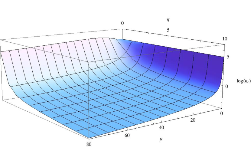
Figure 1: $\log n_{c}$ as a function of $\mu$ and $q$ for $\Delta=2$. Every configuration above this surface is unstable.

In Fig. 2, we show the value of $n_{c}$ for $\mu=5$, varying $\Delta$ and $q$. As expected, we see that decreasing $\Delta$ or increasing $q$ makes the configuration less stable. From this graph, we can determine the critical value $\Delta_{c}$ (for a given $q$) at which the instability kicks in. In Fig. 3, we plot the curves $\Delta(q)$ for different values of $n_{c}$ and show that the curves approach the analytic value derived in (41) as $n_{c}\to\infty$. This confirms the effective mass analysis given above.

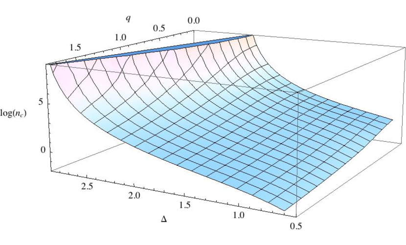
Figure 2: The graph of $\log n_{c}$ as we vary $q$ and $\Delta$ for $\mu=5$. Every configuration above this surface is unstable.

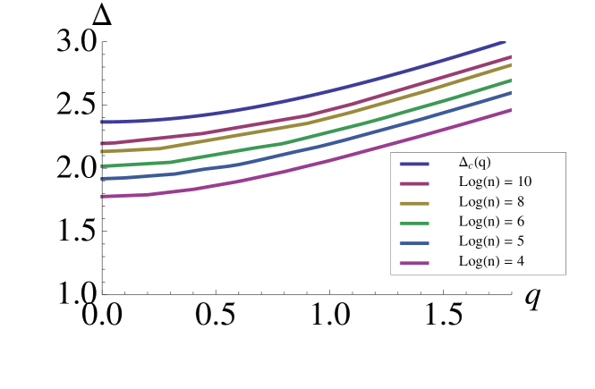
Figure 3: The graph of $\Delta$ as we vary $q$ for $\mu=5$ and different values of $\log n$. As we increase $n$, we get closer and closer to the analytical estimate $\Delta_{c}(q)$.

In Fig. 4, we show the critical chemical potential $\mu_{c}$ as a function of ($\Delta$,$q$) with $n_{c}=1$. We see that, even when $n=1$, it is possible for the Einstein-Maxwell black hole to be unstable. When $\mu>\mu_{c}$, the scalar condenses even though the only remaining defect inserted at the entangling surface is a Wilson line. As we increase $q$ and/or decrease $\Delta$, $\mu_{c}$ decreases. We note, however, that $\mu=0$ is always stable as long as $\Delta$ is above the unitarity bound, $\Delta>1/2$.

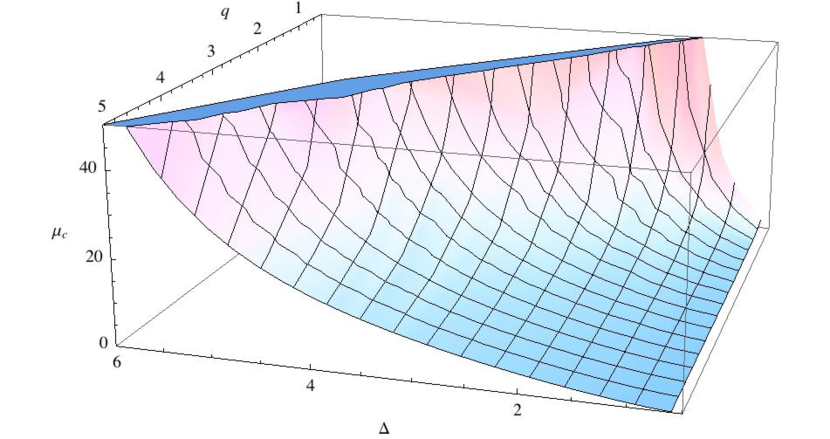
Figure 4: The graph of $\mu_{c}$ as we vary $q$ and $\Delta$ at $n_{c}=1$. Every configuration above this surface is unstable.

4 Discussion

We have shown that the hyperbolic charged black hole can become unstable, and investigated the onset of the instability as we vary $n$, $\mu$ and $\Delta$. We now comment on our results. First, we note that for an uncharged scalar ($q=0$), the black hole can be unstable for sufficiently small scalar mass. This is not surprising; for $\mu\neq 0$ this was already noticed in the holographic superconductor Hartnoll:2008kx for black holes with flat horizons. However, we have seen that for hyperbolic black holes increasing the chemical potential first renders the solution more stable until we reach a peak of stability. Beyond that point, increasing $\mu$ renders the black holes more unstable as can be seen in Fig. 6. This is in contrast with flat black holes, where no condensation can occur for $\mu=0$.

In addition to the numerical method used above, one can also use a WKB method to determine when instabilities exist and to approximate the unstable modes. We will study this in the $q=0$ case, and use the WKB analysis to confirm the surprising behaviour described above. The number of bound states of the Schrodinger potential $V(r^{*})$ can be estimated using the WKB integral:

$$N_{bound~{}states}=\int\sqrt{-V(r^{*})}dr^{*}=\int_{rh}^{r0}\frac{\sqrt{-V(r)}}{f(r)}dr$$ (44)

where we integrate from the horizon $r=r_{h}$ up to the zero of the potential $V(r_{0})=0$, with $r_{0}>r_{h}$. The instability appears when $N_{bound~{}states}\sim 1$. Keeping the temperature fixed and increasing $\mu$, we find $N_{bound~{}states}$ first decreases and then increases again as we increase $\mu$. We plot of $\int\sqrt{-V(r^{*})}dr^{*}$ against $\mu$ at $\Delta=2$ at 10 different temperatures in Fig. 5 below. One can see that for a given $n$ it decreases with $\mu$ before increasing again for sufficiently large $\mu$, signifying that the system is more stable as $\mu$ increases at small $\mu$, but the trend is reversed for larger values of $\mu$. As a note of caution however, we emphasize that – in the absence of any small perturbative parameter – this WKB approximation should at best be taken with a grain of salt, although it does reproduce the qualitative features of the numerics.

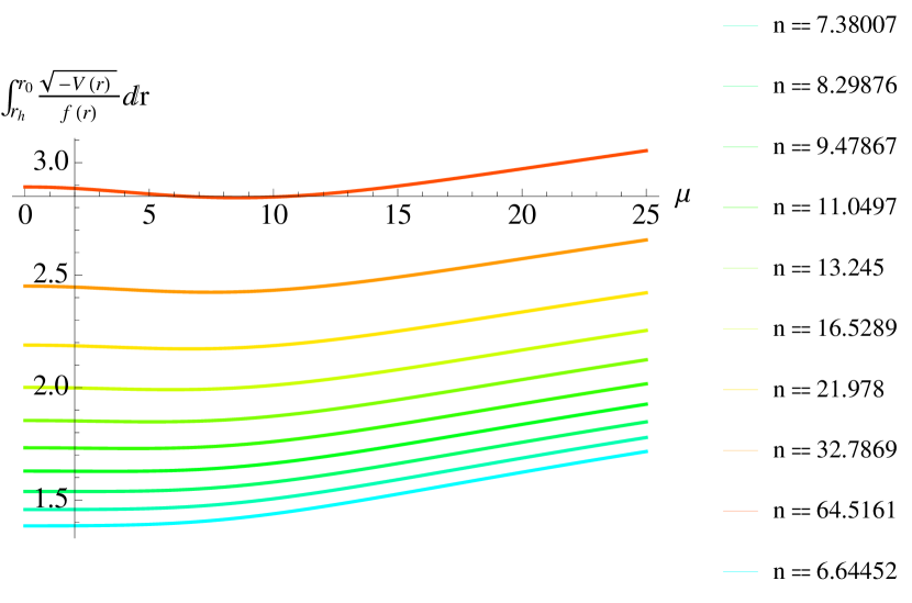
Figure 5: Plots of $\int_{r_{h}}^{r_{0}}\sqrt{-V(r)}/f(r)dr$ against $\mu$ at $\Delta=2$ at 10 different temperatures.

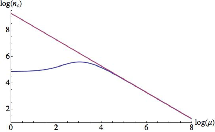
Figure 6: The graph of $\log n_{c}$ as we vary $\mu$ for $q=0$ and $\Delta=2$. The blue line represents the critical Rényi parameter and the red line represents the critical temperature for the field theory on flat space with physical chemical potential $\mu$.

Next, we would like to comment on the large $\mu$ limit of the charged Rényi entropies. When $\mu$ becomes larger than any other scale in the problem, the critical temperature should be proportional to $\mu$. One should note however, that the ratio $T/\mu$ remains small even in the scaling regime, meaning that the black hole continues to stay close to extremality, an observation also noted in the flatly sliced AdS charged black holes Hartnoll:2008kx . This is indeed the case as can be seen in Fig. 6.

It is interesting to compare the critical temperature of the charged hyperbolic black hole with that of its flat counterpart – the flat holographic superconductor at finite (physical) chemical potential $\mu$. We find a perfect match for large $\mu$; this is to be expected, since when $\mu/R\gg 1/L$ the curvature of the horizon is small compared to the scale set by the chemical potential. This can be seen in Fig. 6 as well. We note that, although the gravitational computations for flat and hyperbolic black holes are quite similar, these quantities have very different CFT interpretations. In particular, we see that one can extract information about physical phase transitions at finite chemical potentials and temperatures (which naturally involve higher excited states) solely by considering the entanglement of the ground state.

We should comment on the difference between these two phase transitions from the CFT perspective. The superconductor lives on an infinite flat plane and boundary effects do not play any important role. However, boundary effects at the entangling surface are crucial in the phase transitions of the neutral Rényi entropies, as explained in sachdevON . In the phase transitions of the charged Rényi entropies, there is a qualitative difference between the neutral and the charged scalar operators. As in the case of the neutral Rényi entropies, neutral operators can be hosted on the entangling surface without breaking the $U(1)$ symmetry. Below the critical temperature, these localized operators induce the phase transitions. There is another instability, which is caused by the entanglement chemical potential term coupling to the entire subsystem. As in the case of the superconductors, this instability causes the scalar to condense as well. These two effects may in principle compete or amplify one another. On the other hand, charged operators cannot be hosted on the entangling surface unless the $U(1)$ symmetry is spontaneously broken. Therefore, it is the entanglement chemical potential effect that causes the phase transition. This could explain the qualitative difference in the phase transitions between the $q=0$ case and the $q\neq 0$ case (as shown in Fig.1). This would be interesting to investigate from the field theory point of view.

Let us comment also on the $n=1$ limit. When $n=1$ and $\mu=0$ the conical defect operator disappears and we obtain the entanglement entropy. On the other hand, if $\mu$ is non-vanishing, then even as $n\to 1$ a defect operator – the Wilson line – remains. So a phase transition could occur even at $n\leq 1$. One might worry that a phase transition precisely at $n=1$ would make it impossible to compute entanglement entropies as a limit of the charged Rényi entropies. However, since ${\partial S_{n}\over\partial n}$ is still continuous (only ${\partial^{2}S_{n}\over\partial n^{2}}$ is discontinuous) the Rényi entropies are still smooth enough to give unique and well-defined entanglement entropies as $n\to 1$.

We note also that the Wilson line couples to the global current, so at first sight one might expect it not to effect uncharged operators. We have seen, however, that this is not the case. While uncharged operators do not directly couple to the Wilson line, they still experience its presence indirectly via couplings to other charged operators. This is manifested holographically by the fact that even neutral scalar fields in the bulk can detect changes in $\mu$ at fixed temperature indirectly, via the $\mu$ dependence of the metric.

One can also extract information about the largest eigenvalue of the charged reduced density matrix (11) by considering the limit $n\to\infty$. From the definition of the Rényi entropy (2), one can compute the eigenvalues of the charged reduced density matrix (11) once we know the Rényi entropy as a function of the Rényi parameter $n$;

$$\exp((1-n)S_{n})=\int_{0}^{\lambda_{1}}d\lambda~{}d(\lambda)\lambda^{n}$$ (45)

where $\lambda$ is the eigenvalue and $d(\lambda)$ is the spectral density. $\lambda_{1}$ is the largest eigenvalue. In general, $d(\lambda)$ contains delta functions. In fact, if the Rényi entropy decays polynomially as $n\to\infty,$ one can show that the spectral function take the following form

$$d(\lambda)=\delta(\lambda-\lambda_{1})h_{1}(\lambda)+\Theta(\lambda-\lambda_{1})h_{2}(\lambda),$$ (46)

where $h_{1}$ and $h_{2}$ are some functions of $\lambda$ and $\Theta(\lambda-\lambda_{1})$ is the Heaviside step function. There is a simple relation between the largest eigenvalue $\lambda_{1}$ and the $n\to\infty$ limit of the Rényi entropy (called the min-entropy)

$$S_{\infty}=-\log\lambda_{1}.$$ (47)

Below the critical temperature (when $n>n_{c}$) the scalar field acquires a non-zero expectation value. These hairy black holes have smaller thermal entropy than that of non-hairy black holes of the same temperature and chemical potential. Since the Rényi entropy is given by the integral of the thermal entropy (15), this means that the min-entropy $S_{\infty}$ is always smaller than that of Einstein-Maxwell black hole

$$S_{\infty}(\text{Einstein-Maxwell})>S_{\infty}(\text{Einstein-Maxwell-Scalar})$$ (48)

Moreover, the critical temperature increases as one decreases the conformal dimension $\Delta$. Therefore, as observed in Belin:2013dva ,

$${dS_{\infty}(\mu,\Delta)\over d\Delta}>0.$$ (49)

The main difference between the neutral case Belin:2013dva and the charged case is that (49) is a strict inequality even in the case of $n_{c}\leq 1$, while the neutral case is not. Therefore $S_{\infty}(\mu,\Delta)$ is a monotonic function of $\Delta$. The entanglement chemical potential dependence of the min-entropy is

$${dS_{\infty}(q\neq 0,\Delta)\over d\mu}<0.$$ (50)

We close by recalling that the chemical potential in hyperbolic space can be interpreted as the insertion of a background Wilson line. The insertion of the Wilson line in the imaginary time direction has opposite orientation when viewed from region $A$ as opposed to its complement $B$. At the same time, the ground state satisfies $S_{n}(A)=S_{n}(B)$, for all $n$, since the reduced density matrices of $A$ and $B$ have the same eigenvalues. Thus

$$S_{n}(\mu,A)=S_{n}(-\mu,B).$$ (51)

In a theory with charge conjugation invariance, this would additionally imply that $S_{n}(\mu,A)=S_{n}(-\mu,A)$, i.e. that the charged Rényi entropy is an even function of $\mu$. This is, in particular, clearly true in the case of holographic dual of Einstein-Maxwell theory.

References

-
(1)
M. Levin and X.-G. Wen,
“Detecting Topological Order in a Ground State Wave Function,”
Phys. Rev. Lett. 96 (2006) 110405
[arXiv:cond-mat/0510613];
A. Kitaev and J. Preskill, “Topological entanglement entropy,” Phys. Rev. Lett. 96 (2006) 110404 [arXiv:hep-th/0510092];
A. Hamma, R. Ionicioiu and P. Zanardi, “Ground state entanglement and geometric entropy in the Kitaev’s model,” Phys. Lett. A 337 (2005) 22 [arXiv:quant-ph/0406202]. -
(2)
P. Calabrese and J. L. Cardy,
“Entanglement entropy and quantum field theory,”
J. Stat. Mech. 0406, P002 (2004)
[arXiv:hep-th/0405152];
P. Calabrese and J. L. Cardy, “Entanglement entropy and quantum field theory: A non-technical introduction,” Int. J. Quant. Inf. 4, 429 (2006) [arXiv:quant-ph/0505193]. - (3) D. N. Kabat and M. J. Strassler, “A Comment on entropy and area,” Phys. Lett. B 329, 46 (1994) [hep-th/9401125].
-
(4)
S. Ryu and T. Takayanagi,
“Holographic derivation of entanglement entropy from AdS/CFT,”
Phys. Rev. Lett. 96 (2006) 181602
[arXiv:hep-th/0603001];
S. Ryu and T. Takayanagi, “Aspects of holographic entanglement entropy,” JHEP 0608 (2006) 045 [arXiv:hep-th/0605073];
T. Nishioka, S. Ryu and T. Takayanagi, “Holographic Entanglement Entropy: An Overview,” J. Phys. A 42 (2009) 504008 [arXiv:0905.0932 [hep-th]];
T. Takayanagi, “Entanglement Entropy from a Holographic Viewpoint,” arXiv:1204.2450 [gr-qc]. -
(5)
M. Van Raamsdonk,
“Comments on quantum gravity and entanglement,”
arXiv:0907.2939 [hep-th];
M. Van Raamsdonk, “Building up spacetime with quantum entanglement,” Gen. Rel. Grav. 42 (2010) 2323 [arXiv:1005.3035 [hep-th]]. - (6) R. Horodecki, P. Horodecki, M. Horodecki and K. Horodecki, “Quantum entanglement,” Rev. Mod. Phys. 81, 865 (2009) [quant-ph/0702225].
- (7) D. D. Blanco, H. Casini, L. -Y. Hung and R. C. Myers, “Relative Entropy and Holography,” JHEP 1308, 060 (2013) [arXiv:1305.3182 [hep-th]].
- (8) J. Bhattacharya, M. Nozaki, T. Takayanagi and T. Ugajin, “Thermodynamical Property of Entanglement Entropy for Excited States,” Phys. Rev. Lett. 110, no. 9, 091602 (2013) [arXiv:1212.1164].
- (9) A. Belin, L. -Y. Hung, A. Maloney, S. Matsuura, R. C. Myers and T. Sierens, “Holographic Charged Renyi Entropies,” JHEP 1312, 059 (2013) [arXiv:1310.4180 [hep-th]].
- (10) T. Nishioka and I. Yaakov, “Supersymmetric Rényi Entropy,” JHEP 1310, 155 (2013) [arXiv:1306.2958 [hep-th]]. T. Nishioka, “The Gravity Dual of Supersymmetric Renyi Entropy,” arXiv:1401.6764 [hep-th].
- (11) L. -Y. Hung and S. Matsuura [To appear soon]
- (12) A. Belin, A. Maloney and S. Matsuura, “Holographic Phases of Renyi Entropies,” JHEP 1312, 050 (2013) [arXiv:1306.2640 [hep-th]].
- (13) M.A. Metlitski, C.A. Fuertes, and S. Sachdev “Entanglement Entropy in the O(N) model”, Phys. Rev. B 80, 115122 (2009) [arXiv:0904.4477 [cond-mat]],
- (14) J.M. Stephan, G. Misguich, and V.Pasquier, “Phase transition in the Rényi-Shannon entropy of Luttinger liquids” Phys.Rev.B 84, 195128 (2011) [arXiv:1104.2544]
- (15) H. Casini, M. Huerta and R. C. Myers, “Towards a derivation of holographic entanglement entropy,” JHEP 1105 (2011) 036 [arXiv:1102.0440 [hep-th]].
- (16) L.-Y. Hung, R. C. Myers, M. Smolkin and A. Yale, “Holographic Calculations of Renyi Entropy,” JHEP 1112 (2011) 047 [arXiv:1110.1084 [hep-th]].
- (17) G. Pastras and D. Manolopoulos, arXiv:1404.1309 [hep-th].
- (18) S. A. Hartnoll, C. P. Herzog and G. T. Horowitz, “Building a Holographic Superconductor,” Phys. Rev. Lett. 101, 031601 (2008) [arXiv:0803.3295 [hep-th]]; S. A. Hartnoll, C. P. Herzog and G. T. Horowitz, “Holographic Superconductors,” JHEP 0812, 015 (2008) [arXiv:0810.1563 [hep-th]].
- (19) S. S. Gubser, “Breaking an Abelian gauge symmetry near a black hole horizon,” Phys. Rev. D 78, 065034 (2008) [arXiv:0801.2977 [hep-th]].
- (20) H. Li, , and F. D. M. Haldane, “Entanglement Spectrum as a Generalization of Entanglement Entropy: Identification of Topological Order in Non-Abelian Fractional Quantum Hall Effect States,” Physical Review Letters, 101, 010504 (2008) [arXiv:0805.0332].
- (21) T. H. Hsieh and L. Fu, “Bulk Entanglement Spectrum Reveals Quantum Criticality within a Topological State,” [arXiv:1305.1949].
- (22) S. Ryu and T. Takayanagi, “Holographic derivation of entanglement entropy from AdS/CFT,” Phys. Rev. Lett. 96, 181602 (2006) [hep-th/0603001]; “Aspects of Holographic Entanglement Entropy,” JHEP 0608, 045 (2006) [hep-th/0605073]; T. Nishioka, S. Ryu and T. Takayanagi, “Holographic Entanglement Entropy: An Overview,” J. Phys. A 42, 504008 (2009) [arXiv:0905.0932 [hep-th]].
- (23) M. Headrick, “Entanglement Renyi entropies in holographic theories,” Phys. Rev. D 82, 126010 (2010) [arXiv:1006.0047 [hep-th]]; T. Faulkner, “The Entanglement Renyi Entropies of Disjoint Intervals in AdS/CFT,” arXiv:1303.7221 [hep-th]; A. Lewkowycz and J. Maldacena, “Generalized gravitational entropy,” arXiv:1304.4926 [hep-th].
- (24) D. V. Fursaev, “Proof of the holographic formula for entanglement entropy,” JHEP 0609, 018 (2006) [hep-th/0606184]; D. V. Fursaev, “Entanglement Renyi Entropies in Conformal Field Theories and Holography,” JHEP 1205, 080 (2012) [arXiv:1201.1702 [hep-th]].
- (25) O. J. C. Dias, R. Monteiro, H. S. Reall and J. E. Santos, “A Scalar field condensation instability of rotating anti-de Sitter black holes,” JHEP 1011, 036 (2010) [arXiv:1007.3745 [hep-th]].
- (26) A. Lewkowycz and J. Maldacena, JHEP 1308, 090 (2013) [arXiv:1304.4926 [hep-th]].
- (27) S. S. Gubser and I. Mitra, hep-th/0009126. S. S. Gubser and I. Mitra, JHEP 0108, 018 (2001) [hep-th/0011127].
- (28) C. Martinez, R. Troncoso and J. Zanelli, Phys. Rev. D 70, 084035 (2004) [hep-th/0406111].