Inverse cascade of non-helical magnetic turbulence in a relativistic fluid

Abstract

The free decay of non-helical relativistic magnetohydrodynamic turbulence is studied numerically, and found to exhibit cascading of magnetic energy toward large scales. Evolution of the magnetic energy spectrum $P_{M}(k,t)$ is self-similar in time and well modeled by a broken power law with sub-inertial and inertial range indices very close to $7/2$ and $-2$ respectively. The magnetic coherence scale is found to grow in time as $t^{2/5}$, much too slow to account for optical polarization of gamma-ray burst afterglow emission if magnetic energy is to be supplied only at microphysical length scales. No bursty or explosive energy loss is observed in relativistic MHD turbulence having modest magnetization, which constrains magnetic reconnection models for rapid time variability of GRB prompt emission, blazars and the Crab nebula.

1. Introduction

Freely decaying magnetohydrodynamic (MHD) turbulence is a phenomenon of fundamental importance within the theory of magnetized fluids. That its operation may include the cascading of energy toward larger scales bears far-reaching implications in cosmology and high-energy astrophysics. For example, the strength and coherence scale of the present-day galactic magnetic field could be explained by inverse cascading from extremely small scale fields seeded by phase transitions in the early universe (Field & Carroll, 2000; Tevzadze et al., 2012). Inverse cascading of magnetic energy could also explain recent measurements of strong optical polarization in gamma-ray burst (GRB) afterglows (Uehara et al., 2012; Mundell et al., 2013), where magnetic energy production is believed to operate only at very small scales.

Turbulent inverse cascades are associated with the accumulation of energy at wavelengths longer than the turbulence integral scale. They entail the self-organization of turbulent structures, wherein order emerges from chaotic initial conditions. A familiar example is that of two-dimensional hydrodynamic turbulence, where inverse cascading of kinetic energy is a consequence of global enstrophy conservation. Inverse cascades are qualitatively distinct from direct cascades in that they shift energy away from, rather than toward the dissipation scale. In general, turbulent energy flux moves in both directions. But in three-dimensional hydrodynamic turbulence, modes above the integral scale are damped by instabilities faster than they are pumped by motions in the inertial range.

Since the work of Frisch et al. (1975) it has been well appreciated that MHD turbulence may exhibit inverse cascading as a consequence of global magnetic helicity conservation. But the literature to date is still conflicted on whether helicity is a necessary condition for inverse cascading to occur. It was shown by Olesen (1997) and Shiromizu (1998) that inverse cascading could be expected even for non-helical configurations, as a consequence of rescaling symmetries native to the Navier-Stokes equations. But no inverse cascading was seen in numerical studies based on EDQNM theory (Son, 1999) or direct numerical simulations with relatively low resolution (Christensson et al., 2001; Banerjee & Jedamzik, 2004). Given that mechanisms for helicity production in the early universe are uncertain, and completely absent from regions of GRB afterglow emission, it is crucial to understand the operation of freely decaying non-helical MHD turbulence.

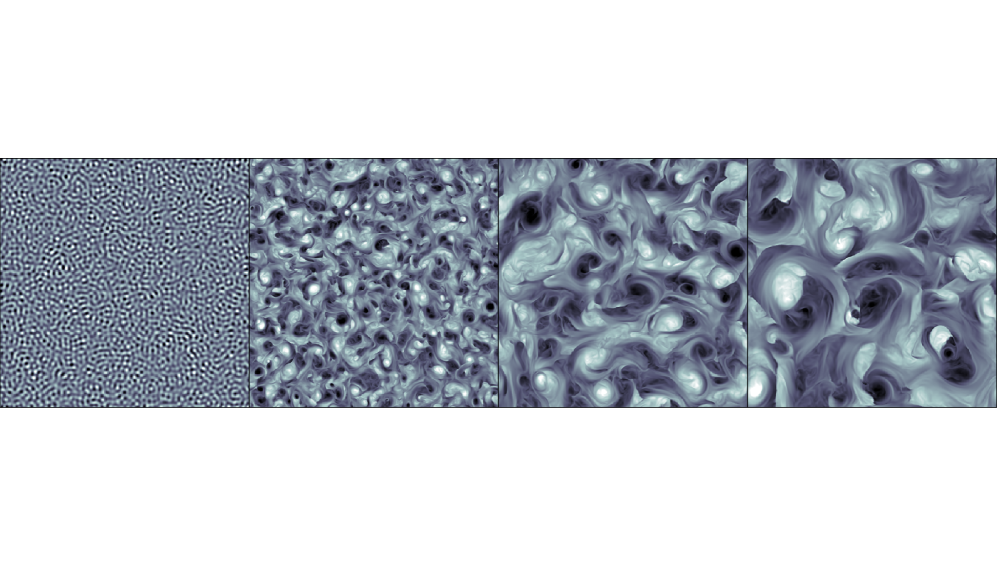
Figure 1.— Two-dimensional slices of transverse magnetic field component showing the progression of magnetic field decay in a three-dimensional relativistic MHD turbulence. The left-most panel shows the initial condition, and then from left to right the solution is shown at 4, 32, and 128 initial Alfvén crossing times of the simulation domain.

In this Letter we establish that helicity is not a necessary condition for inverse cascading in relativistic MHD turbulence. The intended domains of applicability are the evolution of primordial magnetic fields, and those thought to be responsible for the synchrotron emission of GRB afterglows. Given that neither is free of relativistic complications, our results are based on numerical solutions of the relativistic MHD equations. We adopt the initial value problem $P_{M}(k,0)\propto\delta(k-k_{0})$, where $k_{0}^{-1}$ is much smaller than the simulation domain ($P_{M}(k,t)$ is defined so that the electromagnetic energy density $E_{M}(t)=\int P_{M}(k,t)~{}dk$). This choice is permits the system to evolve toward a universal energy spectrum, allowing the sub-inertial and inertial range indices to be measured instead of imposed.

Numerical simulations exhibiting inverse cascades in non-helical, non-relativistic MHD turbulence were reported by Brandenburg et al. (2014) concurrently with the preparation of this work. Our treatment goes farther by including relativistic effects, and by proposing a self-similar ansatz for the evolution of $P_{M}(k,t)$ which agrees very closely with the simulation results. We have studied freely decaying MHD turbulence, whereas Brandenburg et al. (2014) assumed continuous magnetic energy injection at small scales. Despite these differences, both studies support the existence of inverse magnetic energy transfer in non-helical MHD turbulence. The case of relativistic MHD turbulence driven continuously at large scales as been treated previously (Zrake & MacFadyen, 2011, 2013). Our numerical setup is described in Section 2. Simulation results and our self-similar ansatz are given in Section 3. In Section 4.3 we suggest a phenomenological picture that accounts for inverse cascading of MHD turbulence. We also draw comparisons with previous numerical and analytical work in Section 4.1, and in Section 4.2 examine the generality of the initial value problem chosen for this study. Finally, in Section 4.4 we discuss the implications of our findings to the physics of GRB prompt and afterglow emission.

2. Numerical set-up

The scenario investigated here is described as follows. Consider a perfectly conducting fluid whose rest mass, thermal, and magnetic energy densities are mutually comparable. Assume that the magnetic field has periodicity scale $L$, is out of equilibrium such that $\mathbf{J}\times\mathbf{B}\neq 0$, is non-helical, and has an energy spectrum $P_{M}(k,0)$ that is peaked at the scale $k_{0}\gg 2\pi/L$. Time-dependent solutions of the relativistic MHD equations

$$\nabla_{\nu}\rho u^{\mu} =0$$ (1a)

$$\nabla_{\nu}T^{\mu\nu} =0$$ (1b)

$$\frac{\partial\mathbf{B}}{\partial t} =\mathbf{\nabla}\times(\mathbf{v}\times\mathbf{B})$$ (1c)

are obtained using the Mara code (Zrake & MacFadyen, 2011) run on a three-dimensional computational mesh with $512$ grid points along each axis. In Equation 1, $T^{\mu\nu}$ is the stress-energy tensor including both hydrodynamic and electromagnetic contribution, $u^{\mu}$ is the fluid four-velocity, and $\rho$ is mass density. The magnetic field is initially divergenceless and Gaussian-random with a power spectrum that is narrowly peaked around the wavenumber $k_{0}=50k_{1}$, where $k_{1}=2\pi/L$. $P_{M}(k,t)$ is normalized so that the plasma-$\beta$, the ratio of gas to magnetic pressure, is initially $1$.

We define inverse cascading as the accumulation of energy in the sub-inertial range modes (those above the turbulence integral scale), which is evident when the magnetic energy spectrum $P_{M}(k,t)$ is an increasing function of time for wavenumbers $k<k_{t}$ where $k_{t}$ is integral scale wavenumber at time $t$. Note that migration of $k_{t}$ toward smaller values over time is not a sufficient condition for inverse cascading; growth of the coherence scale also occurs in so-called “selective decay”, whereby energy is processed through a direct cascade that drains energy in the small scales before the larger. Interestingly, both processes have been suggested to involve leftward migration of $k_{t}$ depending upon time like $t^{-2/5}$ (Olesen, 1997; Shiromizu, 1998; Son, 1999).

3. Results

Figure 1 shows two dimensional slices of the out-of-page magnetic field component taken at roughly logarithmic intervals throughout the simulation. The left-most panel shows the initial Gaussian-random magnetic field configuration. The second panel shows the solution after a single Alfvén crossing time of the simulation domain, during which the field has organized itself into a collection of small magnetic islands having complex internal structure. The third and fourth panels show those islands becoming larger in scale, and less numerous. The color mapping has been stretched to the minimum and maximum data values of each image, so only the field morphology is depicted and not its average magnitude. Since the initial condition lacks magnetic energy at large scales, the appearance of larger coherent magnetic field structures cannot be selective decay, but can only be attributed to the inverse transfer of magnetic energy from small to large scales.

Indeed, as shown in Figure 2 the magnetic energy spectrum $P_{M}(k,t)$ is an increasing function of time for small $k$ at early times. For each wavenumber $k<k_{0}$, there is a turn-over time $\tau_{k}$ when $\frac{\partial}{\partial t}P_{M}(k,t)$ switches sign. $\tau_{k}$ is thus the time when coherent magnetic field structures of wavenumber $k$ are fully developed, and captures the time required for the magnetic field to assemble itself at length scale $k^{-1}$. At times $t>\tau_{k}$, the amplitude of wavenumber $k$ structures diminishes as a power law in time, $P_{M}(k,t)\propto t^{\delta}$ where $\delta$ is measured to be $-1.3\pm 0.03$. The fiducial value of $-4/3$ will be adopted for simplicity.

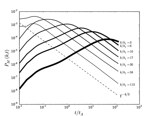
Figure 2.— The temporal evolution of $P_{M}(k,t)$ at seven representative wavenumbers. Heavier ink denotes larger scales. The dashed line shows a power law with index $-4/3$

Figure 3 shows $P_{M}(k,t)$ at several times throughout the simulation. After a fraction of an Alfvén time, the magnetic energy spectrum relaxes to a form which is well described by a split power law

$$P_{M}(k,t_{A})\propto\begin{cases}\left(\frac{k}{k_{0}}\right)^{\alpha}&k<k_{0}\\ \left(\frac{k}{k_{0}}\right)^{\beta}&k\geq k_{0}\end{cases}.$$ (2)

where the sub-inertial and inertial range indices are measured to be $\alpha=3.50\pm 0.04$ and $\beta=-1.91\pm 0.005$ respectively. The values $\alpha=7/2$ and $\beta=-2$ will be adopted for simplicity. We note here that the magnetic energy spectrum is found to be significantly steeper than $5/3$ as is predicted in the Goldreich-Sridhar (Goldreich & Sridhar, 1995) phenomenology. $5/3$ scaling has been verified numerically in strong Alfvén wave turbulence as well as isotropic MHD turbulence driven kinetically at large scales (see e.g. Tobias et al., 2011, for a review). However, it appears that isotropic, freely decaying MHD turbulence has a slope that is significantly steeper than is predicted by the Goldreich-Sridhar theory.

As shown in the upper panel of Figure 4, the break in the power spectrum lies at $k_{t}\propto t^{\gamma}$ where $\gamma$ is consistent with the value of $-2/5$ predicted by scaling arguments made in Shiromizu (1998) and Olesen (1997).

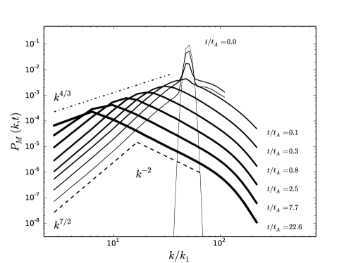
Figure 3.— $P_{M}(k,t)$ shown at nine representative times, including $t=0$ and proceeding through $t=22.6t_{A}$ with lines of increasing width. The dashed lines show power laws with indices $3.5$ and $-2$ for the scales larger and smaller than the injection scale $2\pi/k_{0}$ respectively. The dashed-dotted line shows $P_{M}(k,\tau_{k})\propto k^{4/3}$.

Throughout the simulation, the sub-inertial and inertial range indices remain fixed, with the peak of magnetic energy moving down and to the left on the axes of Figure 3. In other words, the evolution of the magnetic energy spectrum is very nearly self-similar, being well-described by

$$P_{M}(k,t)=s^{\gamma\beta+\delta}P_{M}(ks^{-\gamma},t_{A})$$ (3)

where $s=t/t_{A}$ and $\delta=-4/3$ is the power-law index for decay at all wavenumbers larger than $k_{t}$, as shown in Figure 2. In this empirical model the magnetic energy at each scale larger than $k_{t}^{-1}$ grows proportionally to $t^{\gamma(\beta-\alpha)+\delta}=t^{13/15}$ and the energy associated with peak magnetic structures, $P_{M}(k_{t},t)$ diminishes as $t^{\gamma\beta+\delta}=t^{-8/15}$. Those peaks trace out $P_{M}(k,\tau_{k})\propto k^{4/3}$ as shown in the dashed-dotted line of Figure 3. In the limit of $Lk_{t}\rightarrow\infty$ the total magnetic energy $E_{M}(t)\propto t^{\gamma(\beta+1)+\delta}=t^{-14/15}$ as shown in the lower panel of 4.

4. Discussion

4.1. Comparison with other studies

Direct numerical simulation of freely decaying non-helical MHD turbulence have been carried out by Christensson et al. (2001) and Banerjee & Jedamzik (2004) which report selective decay and no inverse cascade. Nevertheless, it is possible that an inverse cascade was present, but hidden beneath the sub-inertial part of the imposed energy spectrum, for which indices of $2$ and $4$ were chosen by each study respectively. It was observed here that the locus of peak spectral energy $P_{M}(k,\tau_{k})\propto k^{4/3}$, so additional scale separation might have been required in those studies for an inverse cascade to become apparent. Our results are in general agreement with those of Brandenburg et al. (2014), which are based on direct numerical simulations of non-helical, non-relativistic MHD turbulence done with very high resolution. That study reported a slightly steeper slope of the sub-inertial range.

Inverse cascading of magnetic energy in the test-field limit was also reported very recently by Berera & Linkmann (2014). This study found that passive vector fields advected within fully developed, isotropic hydrodynamic turbulence attain coherency over increasing sptial scales. This discovery offers an interesting avenue to examining the generality of inverse cascading.

The inverse cascading observed in our study is not the result of residual helicity in the initial data. Helicity conservation requires only that the correlation scale $k_{t}^{-1}$ is larger than $k_{M}^{-1}=H_{M}/E_{M}$ (Tevzadze et al., 2012). But in our study $k_{M}^{-1}$ evolves from $1/1000$ of the grid spacing up to roughly the grid spacing throughout the simulation. So in fact the correlation scale $k_{t}^{-1}$ remains at least 1000 times larger than the lower limit imposed by helicity conservation throughout the simulation.

4.2. Generality of the initial value problem

We have found that inverse cascading of magnetic energy proceeds from the initial value problem $P_{M}(k,0)\propto\delta(k-k_{0})$. After a fraction of an Alfvén time, the spectrum relaxes toward the split power law in Equation 2. Subsequent enhancement of magnetic energy at scales larger than $k_{t}^{-1}$ occurs through self-similar evolution of the split power solution. Thus inverse cascading must also occur for any initial value problem $P_{M}(k,0)$ which first evolves toward the split power-law solution. Initial value problems where $P_{M}(k,0)$ has non-compact support have also been considered. Olesen (1997) predict that inverse cascading from power-law initial data occurs if and only if the sub-inertial range index $\alpha>-3$, regardless of the magnetic helicity. Verifying this claim numerically will be the topic of a future study.

4.3. Phenomenological picture

We propose that inverse cascading manifests as “unwinding” and “re-linking” of the magnetic field lines. Unwinding refers to the field’s preference for configurations in which the tension force $\mathbf{B}\cdot\nabla\mathbf{B}$ is more uniformly distributed in space. Re-linking occurs where magnetic field loops sourced by parallel line currents attract one another by their mutual Lorentz force $\mathbf{J}\times\mathbf{B}$. This brings regions of opposing magnetic flux into contact with one another creating X-point reconnection sites. At those sites the two flux loops are joined into a single one shaped like a peanut, which then tries to attain maximal average curvature by deforming itself into a circle. This process has the distinct effect of assembling coherent magnetic structures over progressively larger scales, and is insensitive to the mutual linking between flux loops, i.e. the magnetic helicity.

In this scenario inverse magnetic energy transfer cannot be avoided, but its efficiency depends inversely upon the energy lost by the magnetic field during and immediately after the reconnection event. Some portion of magnetic energy is thermalized by non-ideal effects at the moment of reconnection, and another portion is transferred to the bulk flow by accelerating fluid away from the reconnection site. Maximal efficiency of the inverse cascade is attained when the expansion of magnetic field loops is fully adiabatic, in which case the magnetic energy density $E_{M}\propto\ell^{-2}$ where $\ell$ is the size of the loop. Since the characteristic size of the loops scales as $\ell\propto t^{2/5}$, the shallowest possible decay law allowed by this model is $E_{M}\propto t^{-4/5}$. That is only marginally shallower than the decay of $t^{-14/15}$ reported here, which is in turn considerably shallower than $t^{-6/5}$ which is expected if all the energy is lost irreversibly to a direct cascade as in Saffman’s law (Saffman, 1967). The steeper $t^{-6/5}$ follows from the assumption that a fixed fraction of magnetic energy at scale $\ell$ is lost every Alfvén time, which grows as $\sim\ell/v_{A}\propto t^{2/5}E_{M}^{-1/2}$ due to the increasing coherence length and decreasing Alfvén speed.

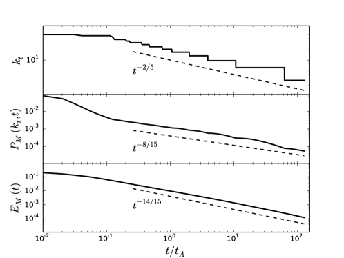
Figure 4.— The upper panel shows the peak wavenumber $k_{t}$ as a function of time, alongside a power law of index $-2/5$ for comparison to analytic predictions. The steps are an artifact of the finite spectral resolution. The middle panel shows $P_{M}(k_{t},t)$ as a function of $t$, and the power law with index $-8/15$ predicted by the empirical model. The lower panel shows the evolution of the average magnetic energy density $E_{M}(t)$, which deviates slightly from the reference slope of $-14/15$ due to the finite value of $Lk_{t}$.

This picture of hierarchical merging of magnetic islands may be consistent with the turbulent reconnection process studied in Lazarian & Vishniac (1999) and Eyink et al. (2011, 2013). Turbulent reconnection predicts small energy losses to direct heating, consistent with what has been reported here. Evidence for low thermalization rates has also been found in recent kinetic simulations of magnetic reconnection across a single current sheet in both relativistic (Sironi & Spitkovsky, 2014) and non-relativistic (Dahlin et al., 2014) plasmas. Those studies show that direct heating caused by parallel electric fields at reconnection sites may be weaker than was previously believed. Instead, the magnetic energy liberated by the change in field topology goes largely into accelerating the bulk flow away from the reconnection site.

4.4. Observational implications

Optical polarization recently detected in GRB afterglows (Uehara et al., 2012; Mundell et al., 2013) requires the magnetic field to attain coherency over the emitting region. If the magnetic field is incoherent immediately behind the shock, the coherence scale would have to grow like $\lambda_{t}\propto t$ to account for the polarized afterglows (Gruzinov & Waxman, 1999). Given that non-helical MHD turbulence has been found to decay with $\lambda_{t}\propto t^{2/5}$, there is simply no way for non-linear evolution of the magnetic field in the downstream region to account for this polarization. If detections of polarized afterglows are to continue, it would be compelling evidence that the magnetic field is already coherent across the emitting region when it is produced at the shock front. This, in turn would favor turbulent dynamo mechanisms for the magnetic energy production (Milosavljevic et al., 2007; Sironi & Goodman, 2007; Goodman & MacFadyen, 2008; Duffell & MacFadyen, 2014) over those based on microphysical plasma instabilities (Gruzinov & Waxman, 1999; Spitkovsky, 2008; Keshet et al., 2009; Sironi & Spitkovsky, 2009; Sironi et al., 2013).

The nature of freely decaying relativistic MHD turbulence, as presented here, also bears implications for the rapid variability of GRB prompt emission (Usov, 1994; Gehrels et al., 2009), blazars (Sikora et al., 2009; Harris et al., 2009, 2011; Hayashida et al., 2012; Bhatta et al., 2013), and the Crab nebula (Tavani et al., 2011; Abdo et al., 2011). The explosive release of magnetic energy by spontaneous magnetic reconnection has also been implicated as a possible mechanism for the flares in GRB prompt emission (Lyutikov & Blandford, 2003; Narayan & Kumar, 2009; Zhang & Yan, 2011; Zhang & Zhang, 2014), blazars (Giannios et al., 2009, 2010; Nalewajko et al., 2011; Calafut & Wiita, 2014; Marscher, 2014), and the Crab nebula (Clausen-Brown & Lyutikov, 2012; Cerutti et al., 2012). However, our simulations, carried out for modest magnetizations with the plasma-$\beta$ initiated at $1$, did not show any indication of bursty or explosive magnetic energy loss; the decay profile is smooth and fluid motions remain slightly below the Alfvén speed at all times. Such behavior is expected given that reconnection in the turbulent fluid takes place over the range of turbulent length-scales.

The absence of reconnection bursts implies that flaring events, if indeed they come from turbulent reconnecting magnetic fields, can only originate in magnetically dominated plasmas if at all. Simulations of freely decaying relativistic, magnetically dominated MHD turbulence are currently being pursued. It is anticipated that in the magnetically dominated case where the Alfvén speed approaches that of light, the turbulent bulk flow will also become relativistic. If so, then models invoking relativistic turbulence (e.g. Narayan & Kumar, 2009) to explain high energy flaring events may remain viable.

References

- Abdo et al. (2011) Abdo, A. A., Ackermann, M., Ajello, M., et al. 2011, Science (New York, N.Y.), 331, 739
- Banerjee & Jedamzik (2004) Banerjee, R., & Jedamzik, K. 2004, Physical Review D, 70, 123003
- Berera & Linkmann (2014) Berera, A., & Linkmann, M. 2014, 5
- Bhatta et al. (2013) Bhatta, G., Webb, J. R., Hollingsworth, H., et al. 2013, Astronomy & Astrophysics, 558, A92
- Brandenburg et al. (2014) Brandenburg, A., Kahniashvili, T., & Tevzadze, A. G. 2014, eprint arXiv:1404.2238
- Calafut & Wiita (2014) Calafut, V., & Wiita, P. J. 2014, eprint arXiv:1407.3687
- Cerutti et al. (2012) Cerutti, B., Werner, G. R., Uzdensky, D. A., & Begelman, M. C. 2012, The Astrophysical Journal, 754, L33
- Christensson et al. (2001) Christensson, M., Hindmarsh, M., & Brandenburg, A. 2001, Physical Review E, 64, 056405
- Clausen-Brown & Lyutikov (2012) Clausen-Brown, E., & Lyutikov, M. 2012, Monthly Notices of the Royal Astronomical Society, 426, 1374
- Dahlin et al. (2014) Dahlin, J. T., Drake, J. F., & Swisdak, M. 2014, 19
- Duffell & MacFadyen (2014) Duffell, P., & MacFadyen, A. 2014, eprint arXiv:1403.6895
- Eyink et al. (2013) Eyink, G., Vishniac, E., Lalescu, C., et al. 2013, Nature, 497, 466
- Eyink et al. (2011) Eyink, G. L., Lazarian, A., & Vishniac, E. T. 2011, The Astrophysical Journal, 743, 51
- Field & Carroll (2000) Field, G., & Carroll, S. 2000, Physical Review D, 62, 103008
- Frisch et al. (1975) Frisch, U., Pouquet, A., Leorat, J., & Mazure, A. 1975, Journal of Fluid Mechanics, 68, 769
- Gehrels et al. (2009) Gehrels, N., Ramirez-Ruiz, E., & Fox, D. B. 2009, Annual Review of Astronomy & Astrophysics, 47, 567
- Giannios et al. (2009) Giannios, D., Uzdensky, D. A., & Begelman, M. C. 2009, Monthly Notices of the Royal Astronomical Society: Letters, 395, L29
- Giannios et al. (2010) —. 2010, Monthly Notices of the Royal Astronomical Society, 402, 1649
- Goldreich & Sridhar (1995) Goldreich, P., & Sridhar, S. 1995, Astrophysical Journal, 438, 763
- Goodman & MacFadyen (2008) Goodman, J., & MacFadyen, A. 2008, Journal of Fluid Mechnanics, 604, 325
- Gruzinov & Waxman (1999) Gruzinov, A., & Waxman, E. 1999, The Astrophysical Journal, 511, 852
- Harris et al. (2009) Harris, D. E., Cheung, C. C., Stawarz, ., Biretta, J. A., & Perlman, E. S. 2009, The Astrophysical Journal, 699, 305
- Harris et al. (2011) Harris, D. E., Massaro, F., Cheung, C. C., et al. 2011, The Astrophysical Journal, 743, 177
- Hayashida et al. (2012) Hayashida, M., Madejski, G. M., Nalewajko, K., et al. 2012, The Astrophysical Journal, 754, 114
- Keshet et al. (2009) Keshet, U., Katz, B., Spitkovsky, A., & Waxman, E. 2009, The Astrophysical Journal Letters, 693, L127
- Lazarian & Vishniac (1999) Lazarian, A., & Vishniac, E. T. 1999, The Astrophysical Journal, 517, 700
- Lyutikov & Blandford (2003) Lyutikov, M., & Blandford, R. 2003, 78
- Marscher (2014) Marscher, A. P. 2014, The Astrophysical Journal, 780, 87
- Milosavljevic et al. (2007) Milosavljevic, M., Nakar, E., & Zhang, F. 2007, eprint arXiv, 0708, 1588
- Mundell et al. (2013) Mundell, C. G., Kopač, D., Arnold, D. M., et al. 2013, Nature, 504, 119
- Nalewajko et al. (2011) Nalewajko, K., Giannios, D., Begelman, M. C., Uzdensky, D. A., & Sikora, M. 2011, Monthly Notices of the Royal Astronomical Society, 413, 333
- Narayan & Kumar (2009) Narayan, R., & Kumar, P. 2009, Monthly Notices of the Royal Astronomical Society: Letters, 394, L117
- Olesen (1997) Olesen, P. 1997, Physics Letters B, 398, 321
- Saffman (1967) Saffman, P. G. 1967, Physics of Fluids, 10, 1349
- Shiromizu (1998) Shiromizu, T. 1998, Physics Letters B, 443, 127
- Sikora et al. (2009) Sikora, M., Stawarz, ., Moderski, R., Nalewajko, K., & Madejski, G. M. 2009, The Astrophysical Journal, 704, 38
- Sironi & Goodman (2007) Sironi, L., & Goodman, J. 2007, The Astrophysical Journal, 671, 1858
- Sironi & Spitkovsky (2009) Sironi, L., & Spitkovsky, A. 2009, The Astrophysical Journal, 698, 1523
- Sironi & Spitkovsky (2014) —. 2014, The Astrophysical Journal, 783, L21
- Sironi et al. (2013) Sironi, L., Spitkovsky, A., & Arons, J. 2013, The Astrophysical Journal, 771, 54
- Son (1999) Son, D. 1999, Physical Review D, 59, 063008
- Spitkovsky (2008) Spitkovsky, A. 2008, The Astrophysical Journal, 682, L5
- Tavani et al. (2011) Tavani, M., Bulgarelli, A., Vittorini, V., et al. 2011, Science (New York, N.Y.), 331, 736
- Tevzadze et al. (2012) Tevzadze, A. G., Kisslinger, L., Brandenburg, A., & Kahniashvili, T. 2012, The Astrophysical Journal, 759, 54
- Tobias et al. (2011) Tobias, S. M., Cattaneo, F., & Boldyrev, S. 2011, eprint arXiv, 1103, 3138
- Uehara et al. (2012) Uehara, T., Toma, K., Kawabata, K. S., et al. 2012, The Astrophysical Journal, 752, L6
- Usov (1994) Usov, V. 1994, Monthly Notices of the Royal Astronomical Society, 267
- Zhang & Yan (2011) Zhang, B., & Yan, H. 2011, The Astrophysical Journal, 726, 90
- Zhang & Zhang (2014) Zhang, B., & Zhang, B. 2014, The Astrophysical Journal, 782, 92
- Zrake & MacFadyen (2011) Zrake, J., & MacFadyen, A. I. 2011, The Astrophysical Journal, 744, 32
- Zrake & MacFadyen (2013) —. 2013, The Astrophysical Journal, 769, L29