Improving estimates of the number of ‘fake’ leptons and other mis-reconstructed objects in hadron collider events: BoB’s your UNCLE

Abstract

We consider current and alternative approaches to setting limits on new physics signals having backgrounds from misidentified objects; for example jets misidentified as leptons, $b\textrm{-jets}$ or photons. Many ATLAS and CMS analyses have used a heuristic “matrix method” for estimating the background contribution from such sources. We demonstrate that the matrix method suffers from statistical shortcomings that can adversely affect its ability to set robust limits. A rigorous alternative method is discussed, and is seen to produce fake rate estimates and limits with better qualities, but is found to be too costly to use. Having investigated the nature of the approximations used to derive the matrix method, we propose a third strategy that is seen to marry the speed of the matrix method to the performance and physicality of the more rigorous approach.

1 Introduction

Many precision measurements and searches for new physics employ signal regions which have a significant source of background coming from ‘fake’ objects. A typical concrete example is that of leptons, which can be faked by a mis-reconstructed jet. Alternatively one can consider jets faking $b\textrm{-jets}$, for which the matrix method was used in ATLAS-CONF-2013-061 , or even faking photons. In this article the term ‘lepton’ shall be used throughout, but all statements made are general to other types of object. Properties whose distributions differ for ‘fake’ and ‘real’ objects have been used to underpin data-driven methods of fake rate estimation, one of the most prevalent of which during the first data-taking run of the LHC has been the so-called ‘matrix method’ ATLAS-CONF-2010-087 used by ATLAS in atlasMMCitation0 ; atlasMMCitation1 ; atlasMMCitation2 ; atlasMMCitation3 ; atlasMMCitation4 ; atlasMMCitation5 ; atlasMMCitation6 ; atlasMMCitation7 ; atlasMMCitation8 ; atlasMMCitation9 ; atlasMMCitation10 ; atlasMMCitation11 ; atlasMMCitation12 ; atlasMMCitation13 ; atlasMMCitation14 ; atlasMMCitation15 ; atlasMMCitation16 ; atlasMMCitation17 ; atlasMMCitation18 ; atlasMMCitation19 ; atlasMMCitation20 ; atlasMMCitation21 ; atlasMMCitation22 ; atlasMMCitation23 ; atlasMMCitation24 ; atlasMMCitation25 ; atlasMMCitation26 ; atlasMMCitation27 ; atlasMMCitation28 , and by CMS in cmsMMCitation0 ; cmsMMCitation1 ; cmsMMCitation2 based, apparently, on a description in Chatrchyan:2012bra .

The matrix method is the first of three ways of determining fake rates that are compared in this paper. We shall sometimes refer to it for short Method A to facilitate easy comparison with the later Methods B and C. (For quick reference see Table 1.)

Method A makes use of the fact that fake and real leptons tend to differ in their degree of ‘isolation’. Using cuts on isolation (and to a lesser extent other variables) leptons are categorised as either ‘tight’ or ‘loose’, the former being largely synonymous with ‘more isolated’ and the latter with ‘less isolated’. In this paper it is shown that the way in which the resulting matrix method derived background estimates are typically used in existing SUSY searches can give rise to confidence limits that are unstable (highly variable) indicating they are making non-optimal use of the data. More specifically, over the course of many independent experiments one expects to find a distribution of limits from Method A which has a larger variance (is more widely spread out) than the distribution of limits coming from Methods B and C discussed later. In addition, Method A can produce unphysically negative estimates for fake rates that should be bounded below by zero.

Method	Cost of computation	Limit quality	Other names
A	low	poor	‘Matrix Method’ ATLAS-CONF-2010-087
B	very high	very good	‘Likelihood Matrix Method’
C	quite low	good	‘BoB Method’

Table 1: An overview of the three methods discussed in this paper, and their relative strengths and weaknesses. ‘Limit quality’ refers to whether ${CL_{s+b}}$ limits tend to have the correct frequentist coverage properties, and also avoid unnecessary over-coverage.

The weaknesses of the matrix method stem from the presence of heuristic, non-mathematical steps in its derivation. Heuristic methods are often useful, but can be problematic if their underlying assumptions are sometimes invalid; we show this is the case with the matrix method. Methods lacking these deficiencies are in principle trivial to construct. In Method B we describe an example of such a method in which a single likelihood is used to perform both the background estimation and the limit setting. Whilst this can be considered the optimal approach, it is shown to be computationally expensive in cases where objects are divided into many categories. In order to marry the best of Methods A and B, we then propose Method C. It is intended that Method C be usable as a drop-in replacement for Method A in the contexts in which the latter has previously been used by ATLAS or CMS. Method C, like Method A, it is partly heuristic (for speed) and so is justified pragmatically. However, careful choice of the approximations it contains allows it to always give physical limits whose distributions very closely resemble the optimal (but prohibitively expensive) Method B.

Note that fake rate estimates in LHC analyses are likely to find themselves being used as part of a ${CL_{s}}$ frequentist limit setting procedures, since these are endemic in ATLAS and CMS papers. Such usage requires a likelihood for a set of parameters given observed data; in the case where one counts events in just one region, it typically takes the form of a Poisson distribution having some mean. Background estimates in an analysis are then interpreted as an auxiliary measurement which constrains this mean through additional terms in the likelihood. In this context, the fake rate ought to be an estimate of the expected number of events from the fake background process in the signal region, given data collected outside of the signal region. This is not strictly adhered to in the matrix methods, and so is one of the general places in which Methods B and C improve on A.

2 Overview of fake estimation procedures and limit setting

Events collected into some signal region are defined in terms of the numbers of leptons they contain. A cut on some measure of quality, for example isolation, distinguishes a given lepton as loose ($l$) or tight ($t$), where ${l}\cup{t}\equiv{\tilde{l}}$ and ${l}\cap{t}=\emptyset$. Each lepton will also be regarded as either real ($r$) or fake ($f$), depending on whether it is a correctly reconstructed lepton, or for example a mis-reconstructed heavy flavour jet. According to the precise selection, a certain number of tight and loose leptons will be required for an object to make it into a signal region – those that do are described as tight events ($T$), and those that do not but could be made to pass the selection for some permutation of $t$ and $l$ on its constituent leptons are denoted as loose events ($L$), where as before ${L}\cup{T}\equiv{\tilde{L}}$ and ${L}\cap{T}=\emptyset$.

A core concept in all methods considered here is that of the real and fake efficiencies, respectively defined to be ${\varepsilon_{r}}\equiv P({t}|{r}{\tilde{l}})$ and ${\varepsilon_{f}}\equiv P({t}|{f}{\tilde{l}})$. For convenience we will also use ${{\bar{\varepsilon}_{r}}}\equiv 1-{\varepsilon_{r}}=P({l}|{r}{\tilde{l}})$ and ${{\bar{\varepsilon}_{f}}}\equiv 1-{\varepsilon_{f}}=P({l}|{f}{\tilde{l}})$. Typically these quantities are measured in additional control regions, and could be subdivided according to kinematic quantities, such as lepton $\maybebmsf{p_{\maybebmsf}{\mathrm{T}}}$. In this text such categories will be labelled ${\omega_{1}},{\omega_{2}},\ldots$, with the efficiencies gaining an additional subscript e.g. $\varepsilon_{{\omega_{1}}{r}}$.

For a given event containing $m$ leptons, each lepton is observed to be either $l$ or $t$, and will have some category $\omega_{i}$. If there are $N_{\omega}$ possible categories for each lepton, then the number of measurable event categories will be ${N_{\Omega}}=(2\times{N_{\omega}})^{m}$. Each of these will correspond to an event that is either $L$ or $T$.

Experimentally, one counts how many events fall into each of the $N_{\Omega}$ sub-regions, yielding the set of integers $\left\{{n_{{\Omega_{i}}}}\right\}$. For the purpose of the physics analysis being performed, one might be interested in the total number of tight events, ${n_{T}}=\sum_{{\Omega_{i}}\subset{T}}{n_{{\Omega_{i}}}}$. Usually this is the quantity with which a limit on the cross section of a new physics model is placed.

The observed numbers of events are often assumed to be the particular values of a Poisson distributed random variable. That is, one can have ${n_{T}}\sim\text{Poiss}\left({\nu_{T}}\right)$; in general the indices on the rate $\nu$ correspond to those on the observation $n$.

2.1 Method A: the “matrix method”

This section attempts to document Method A, the matrix method, in more detail than has previously been done, and in its most general form. As mentioned previously it is a somewhat heuristic method, but its assumptions shall be interpreted on a firmer statistical footing in a subsequent section.

2.1.1 Events with only one lepton

Consider first a simplified scenario where each event has exactly one lepton; $n_{T}$ tight and $n_{L}$ loose events are observed. The key relation is then that

$$\begin{pmatrix}{{\left<{n_{T}}\right>}}\\ {{\left<{n_{L}}\right>}}\end{pmatrix} =\begin{pmatrix}{\varepsilon_{r}}&{\varepsilon_{f}}\\ {{\bar{\varepsilon}_{r}}}&{{\bar{\varepsilon}_{f}}}\end{pmatrix}\begin{pmatrix}n_{R}\\ n_{F}\end{pmatrix},$$ (1)

where $n_{R}$ and $n_{F}$ are the number of the observed events which are real and fake, respectively. In this context, ${{\left<{n_{L}}\right>}}={\mathbb{E}\left[{{n_{L}}|{n_{R}},{n_{F}}}\right]}$, and similarly for ${{\left<{n_{T}}\right>}}$. The result follows by considering the real/fake event counts to be random variables following a Poisson distribution, which are then further divided into tight and loose components according to a binomial distribution using the probabilities contained in the efficiencies.

It can be noted that equation (1) is similar to a relation between the means of Poisson distributions

$$\begin{pmatrix}{\nu_{T}}\\ {\nu_{L}}\end{pmatrix} =\begin{pmatrix}{\varepsilon_{r}}&{\varepsilon_{f}}\\ {{\bar{\varepsilon}_{r}}}&{{\bar{\varepsilon}_{f}}}\end{pmatrix}\begin{pmatrix}{\nu_{R}}\\ {\nu_{F}}\end{pmatrix}.$$ (2)

This is used later when discussing Method B and Method C, but for now we shall proceed with equation (1). This equation may legitimately be inverted

$$\begin{pmatrix}n_{R}\\ n_{F}\end{pmatrix} =\frac{1}{{\varepsilon_{r}}-{\varepsilon_{f}}}\begin{pmatrix}{{\bar{\varepsilon}_{f}}}&-{\varepsilon_{f}}\\ -{{\bar{\varepsilon}_{r}}}&{\varepsilon_{r}}\end{pmatrix}\begin{pmatrix}{{\left<{n_{T}}\right>}}\\ {{\left<{n_{L}}\right>}}\end{pmatrix},$$ (3)

provided that ${\varepsilon_{r}}\neq{\varepsilon_{f}}$. Given the model assumptions that were made, the steps described hitherto all hold water on mathematical grounds. In contrast, the next step that is usually taken to motivate Method A is quite arbitrary, and is justified largely on grounds that it is effective in situations with large numbers of events, rather than because it is meaningful in general. This ‘heuristic’ step consists of the removal of the expectation brackets from the right hand side of equation (3) and the re-interpretation of the terms on its left hand side as a pair of quantities $\hat{n}_{R}$ and $\hat{n}_{F}$ as follows:

$$\begin{pmatrix}\hat{n}_{R}\\ \hat{n}_{F}\end{pmatrix} =\frac{1}{{\varepsilon_{r}}-{\varepsilon_{f}}}\begin{pmatrix}{{\bar{\varepsilon}_{f}}}&-{\varepsilon_{f}}\\ -{{\bar{\varepsilon}_{r}}}&{\varepsilon_{r}}\end{pmatrix}\begin{pmatrix}n_{T}\\ n_{L}\end{pmatrix}.$$ (4)

What are $\hat{n}_{R}$ and $\hat{n}_{F}$? They depend on $n_{T}$ and $n_{L}$ and so are functions of the data, and may be regarded as estimators – but estimators for what? It is shown in Appendix A that under some additional assumptions, and for certain values of $n_{T}$ and $n_{L}$, they turn out to be maximum likelihood estimators for $n_{R}$ and $n_{F}$ given knowledge of $n_{T}$ and $n_{L}$ (i.e. estimators for ${{\left<{n_{R}}\right>}}\equiv{\mathbb{E}\left[{{n_{R}}|{n_{T}},{n_{L}}}\right]}$ and ${{\left<{n_{F}}\right>}}\equiv{\mathbb{E}\left[{{n_{F}}|{n_{T}},{n_{L}}}\right]}$). Nonetheless, and in the absence of anything better, Method A instead uses $\hat{n}_{R}$ and $\hat{n}_{F}$ as estimators for the unknown and unknowable actual rates of real and fake events, $\nu_{R}$ and $\nu_{F}$.

Note that these estimators are sometimes pretty bad as equation (4) allows terms on its left hand side to become unphysically negative. This happens in real analyses (e.g. atlasMMCitation2 ) creating problems that need to be solved by ad-hoc methods. Both Method B and Method C  have the benefit of avoiding such problems.

Finally, Method A obtains its desired goal, the definition of an estimator for the expected number of fake events in the signal region, $\hat{n}_{TF}$, motivated by equation (1) with the replacement $n_{F}\rightarrow\hat{n}_{F}$, where $\hat{n}_{F}$ is the estimator obtained above in (4). This results in:

$${\hat{n}_{TF}} =\frac{{\varepsilon_{f}}}{{\varepsilon_{r}}-{\varepsilon_{f}}}\left({\varepsilon_{r}}(n_{T}+n_{L})-n_{T}\right).$$ (5)

Again, note the problems with this method that, even if ${\varepsilon_{r}}>{\varepsilon_{f}}$ (as must be the case for a useful definition of $t$ and $l$), equation (5) can yield ${\hat{n}_{TF}}<0$, an unphysical result which is symptomatic of the earlier “sleight of hand”.

This concludes our description of how Method A is used in single lepton events to calculate a number which is used as if it were an estimate of the expected rate of fakes in the signal region. We will now describe how the same method is extended for use in events with more than one lepton, which has previously not been documented in detail.

2.1.2 Events with multiple leptons

Consider an event with two leptons, where each lepton can be in one of a number of categories $\{\omega_{i}\}$. One may define quantities such as $n_{tl}$, the number of events with the first lepton tight and the second loose – others are defined similarly. In order to include the possible categories for each lepton, event counts such as $n_{tt}$ must be further subdivided to take into account all combinations:

$$n_{tt} =n_{tt}^{{\omega_{1}}{\omega_{1}}}+n_{tt}^{{\omega_{1}}{\omega_{2}}}+\cdots$$ (6)

$$=\sum_{i,j}n_{tt}^{{\omega_{i}}{\omega_{j}}}.$$ (7)

In this notation, $n_{tt}^{{\omega_{1}}{\omega_{2}}}$ indicates the number of events with two tight leptons, where the first is in category $\omega_{1}$, and the second in ${\omega_{2}}$.

The analogous relation to equation (1) is then

$${\left<{{n_{\mathcal{T}}}_{\beta_{1}\beta_{2}}^{{\omega_{i}}{\omega_{j}}}}\right>} ={{\phi_{\omega_{i}}}_{\beta_{1}}^{\ \alpha_{1}}}{{\phi_{\omega_{j}}}_{\beta_{2}}^{\ \alpha_{2}}}\ {n_{\mathcal{R}}}_{\alpha_{1}\alpha_{2}}^{{\omega_{i}}{\omega_{j}}},\qquad\text{where}$$ (8)

$${{\phi_{\omega_{i}}}_{\{{t},{l}\}}^{\ \{{r},{f}\}}} =P(\{{t},{l}\}|\{{r},{f}\}{\omega_{i}}{\tilde{l}}),$$ (9)

$$\phi_{\omega_{i}} =\begin{pmatrix}{\varepsilon_{{\omega_{i}}{r}}}&{\varepsilon_{{\omega_{i}}{f}}}\\ {{\bar{\varepsilon}_{{\omega_{i}}{r}}}}&{{\bar{\varepsilon}_{{\omega_{i}}{f}}}}\end{pmatrix},$$ (10)

where summation over repeated upper and lower indices is implied where appropriate. The identifier $n$ has been replaced for clarity with the symbols ${n_{\mathcal{T}}}$ and ${n_{\mathcal{R}}}$, depending on whether the accompanying indices pertain to tight/loose-ness, e.g. ${n_{\mathcal{T}}}_{tl}=n_{tl}$, or real/fake-ness, so ${n_{\mathcal{R}}}_{rf}=n_{rf}$. Each Greek lower index of ${n_{\mathcal{T}}}$ hence takes values in $\{t,l\}$, while each Greek lower index of ${n_{\mathcal{R}}}$ takes values in $\{r,f\}$. The index on these indices corresponds to the which lepton is being described; i.e. in equation (10), the value of $\alpha_{2}$ represents whether the second lepton is either real or fake.

The matrix representation for $\phi_{\omega_{i}}$ shown in the last line of equation (10) is not needed to understand this equation, but is required when considering the background estimate for events that are both tight and fake (it is what still identifies this as the “matrix method”, despite the new notation).

The estimate for the expected number of events that are fake is then ${{{\hat{n}}_{\mathcal{T}}}^{F}{}}_{\alpha_{1}\alpha_{2}}$, where

$${{{\hat{n}}_{\mathcal{T}}}^{F}{}}_{\nu_{1}\nu_{2}}=\sum_{i,j}\left({{\phi_{\omega_{i}}}_{\nu_{1}}^{\ \mu_{1}}}{{\phi_{\omega_{j}}}_{\nu_{2}}^{\ \mu_{2}}}\ \zeta_{\mu_{1}\mu_{2}}^{\ \beta_{1}\beta_{2}}\ {{\phi^{-1}_{\omega_{i}}}_{\beta_{1}}^{\ \alpha_{1}}}{{\phi^{-1}_{\omega_{j}}}_{\beta_{2}}^{\ \alpha_{2}}}{n_{\mathcal{T}}}_{\alpha_{1}\alpha_{2}}^{{\omega_{i}}{\omega_{j}}}\right),$$ (11)

where the $\zeta$ object is responsible for defining what is meant by a fake event. For example, if $rr\equiv{R}$ and $\{rf,fr,ff\}\equiv{F}$ then one would choose $\zeta_{12}^{12}=\zeta_{21}^{21}=\zeta_{22}^{22}=1$, and all other components 0. There is in fact a redundancy in the indices, in that all non-zero components have the $i^{\text{th}}$ lower index the same as the $i^{\text{th}}$ upper index. In general therefore, for the case with any number of leptons

$$\zeta_{\mu_{1}\mu_{2}\cdots}^{\ \beta_{1}\beta_{2}\cdots} =\delta_{\mu_{1}}^{\ \beta_{1}}\delta_{\mu_{2}}^{\ \beta_{2}}\cdots h(\beta_{1},\beta_{2},\ldots),$$ (12)

where $\delta_{i}^{\ j}$ is the Kronecker delta, and $h(\beta_{1},\ldots)$ is a function of the indices that is 1 for a fake combination, and 0 for a real combination.

In order to estimate the number of events contained within $\mathcal{\hat{T}}^{F}$, from equation (11), that are tight, one sums the appropriate component(s). For example, a simple analysis selecting final states with exactly two leptons might define ${T}\equiv{t}{t}$ (i.e. the number of tight events would now be denoted $n_{T}\equiv n_{tt}$), and all other possibilities to be ${L}$. In this case the $\mathcal{\hat{T}}^{F}_{{t}{t}}$ component is the estimate of the number of events that are both tight and fake. For the completely general case with events containing arbitrary numbers of leptons, additional terms and indices are added as necessary to the equations in this section.

2.1.3 Limit setting

ATLAS and CMS analyses use the ${CL_{s}}$ method Mistlberger:2012rs to place an upper limit on the event rate (in the sense of the mean of a Poisson distribution, which controls the appearance of events in a signal region) of new physics processes.

In the context of limit setting, the output from the matrix method is treated on a par with those irreducible background components estimated from Monte Carlo simulated (MC) samples. Once the central value is estimated as described in section 2.1, uncertainties in the measured efficiencies, as well as a statistical uncertainty, can be propagated in the usual way by taking a derivative BIPM1995 . The background mean $\bar{b}$ and uncertainty $\sigma_{b}$ are fed into a joint likelihood for the signal and background rates, $\mu$ and $b$, given the number of events observed in the signal region $n_{T}$. In the case with only one background source it takes the form

$$\mathcal{L}(\mu,b|n_{T}) =\text{Poiss}(n_{T};\mu+b)\text{Gauss}(\bar{b};b,\sigma_{b}).$$ (13)

When setting the limit, the nuisance parameter $b$ is profiled away in the usual way to form the test statistic $q_{\mu}$,

$$q_{\mu} =\begin{cases}-2\ln\left(\dfrac{\mathcal{L}\left(\mu,\hat{\hat{b}}|n_{T}\right)}{\mathcal{L}\left(\hat{\mu},\hat{b}|n_{T}\right)}\right)&\mu>\hat{\mu}\\ 0&\\ \end{cases}.$$ (14)

Confidence intervals (${CL_{s}}$ or ${CL_{s+b}}$) at some level can then be formed by following the recipe outlined in Mistlberger:2012rs .

2.2 Method B: An extended likelihood method

Whilst Method A can suffer from under-coverage, as subsequently discussed in Section 3, this can largely be avoided for a purely data-driven background if the full likelihood, including all data used to make the measurement, is used in the limit setting procedure. That is, one should use

$$\mathcal{L}(\mu,\bm{\theta}|n_{t},n_{l},n_{tt},\ldots),$$ (15)

where $\bm{\theta}$ represents the set of nuisance parameters. If the leptons can fall into one of several categories, quantities should be replaced with the separate terms from equation (7). Each of these quantities can be considered as an independent random variable with a Poisson distribution. The means of these Poisson distributions will be denoted as functions of the parameters e.g. $\nu_{tt}^{{\omega_{1}}{\omega_{1}}}(\mu,\bm{\theta})$; the likelihood then factorises and takes a form similar to equation (13)

$$\mathcal{L}(\mu,\bm{\theta}|\ldots,n_{tt}^{{\omega_{1}}{\omega_{1}}},\ldots)=\text{Poiss}(n_{tt}^{{\omega_{1}}{\omega_{1}}};\nu_{tt}^{{\omega_{1}}{\omega_{1}}}(\mu,\bm{\theta}))\cdots P(\bm{\bar{\theta}}|\bm{\theta}).$$ (16)

The final term represents constraints placed on the nuisance parameters by external measurements.

2.2.1 Choice of parameterisation

The efficacy of any likelihood method depends on a sensible choice of parameterisation. The parameterisation must completely describe how events from both signal and background are expected to be divided between the different event categories without over-parameterising. For example, one could directly use $\nu_{tt}^{{\omega_{1}}{\omega_{1}}}$ etc. as the free parameters $\bm{\theta}$, but this would remove all predictive power!

Other researchers likelihoodMMCranmerComm have investigated the possibility of applying a method that uses a similar parameterisation to the matrix method. This parameterisation uses the efficiencies described before, in addition to the rates separated both by object category and real/fake-ness. Whilst this has an advantage of making minimal assumptions about how a given background process distributes itself between these categories, it does lead to a very large parameter space. For example, even with three objects coming from only three possible categories, there are already 80 such parameters (before considering efficiencies). Since any form of prediction will require a maximisation of the likelihood over this input parameter space, and since such global maximisations become computationally more expensive as dimensionality increases, the authors have chosen to use an alternative parameterisation.

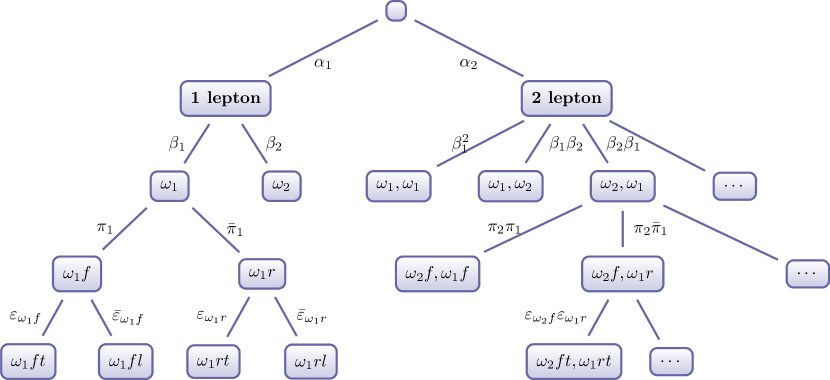
Figure 1: The probability tree in this figure illustrates the model used to parameterise fake and real lepton production, as used in Method B and Method C. The left-most branch is complete, the others are not as indicated by the presence of “…”. In general one could allow both for more lepton categories, as well as more leptons in the event. Note that $\sum_{{m}=0}^{{m}_{\text{max}}}\alpha_{m}=\sum_{i=1}^{N_{\omega}}\beta_{i}=1$, where ${m}_{\text{max}}$ is the largest number of leptons that can be produced in a given event. Additionally, the abbreviation $\bar{\pi}_{i}=1-\pi_{i}$ is used.

Diagrammatically, the parameterisation used in this work is displayed in Figure 1. For every event that is generated, it is first decided how many leptons that event ought to contain. This is controlled by a set of parameters $\{\alpha_{m}\}$, each of which corresponds to the probability of forming an event with $m$ leptons. As noted in the caption, these must sum to 1. For each lepton, a category $\omega_{i}$ is assigned to it with probability $\beta_{i}$, and it is then further assigned to be either $r$ with probability $\pi_{i}$ or $f$ with probability $1-\pi_{i}$. Formally, $\beta_{i}\equiv P({\omega_{i}}|{\tilde{l}})$ and $\pi_{i}\equiv P({f}|{\omega_{i}}{\tilde{l}})$. Efficiencies are then used in the usual way to select objects as being $t$ or $l$.

Using these terms, together with one extra non-negative parameter denoting the mean of the Poisson distribution controlling the total production of tight events, one can compute the terms such as $\nu_{tt}^{{\omega_{1}}{\omega_{1}}}$ in equation (16). It should be noted that one of these trees must exist for every separate ‘component’ that is being fitted – that is, at least one for the hypothesised signal process and one for the fake component of the background, and then optionally one or more for other background components that have been estimated using MC samples.

2.3 Method C: Maximum likelihood estimate

It is later found that Method B is computationally intractable for more than very simple systems. As such, we propose a third method that is found to keep many of the desirable properties of Method B, but also with a much reduced computation time more similar to Method A. This is achieved by using a simple likelihood for limit setting, as in Method A, but feeding it with the true maximum likelihood estimate (MLE) fake rate.

To form an upper limit with Method C, one does the following. Firstly, for the observed data, maximise the likelihood expressed in equation (16) for all nuisance parameters. As mentioned in the discussion for Method B, this likelihood should contain sufficient parameters to describe the signal process, fake background, and any other real backgrounds. The output from this that shall be used is the MLE fake rate with an estimated uncertainty. This uncertainty represents both an uncertainty with which the efficiencies are known, as well as statistical limitations of the observed data. It is estimated with the MINOS method James:1975dr , by taking the values of the fake rate where the minimum of the negative log likelihood with respect to the remaining parameters increases by 0.5 from its minimum value. A limit is then placed using an expression identical to that in equation (13), where $\bar{b}$ and $\sigma_{b}$ take the aforementioned MLE fake rate and uncertainty.

3 Comparisons using frequentist limits

Using a toy event generator, written by the authors, datasets are produced using the same method as that which is depicted in Figure 1, containing a mixture of ‘fake’ and ‘signal’ events. For each of several configurations, 19000 independent datasets were formed using the generator. Each of these was subsequently processed using Methods A, B and C. In all cases the necessary minimisation of a negative log likelihood was performed using the Minuit2 library James:1975dr . The result are 95% ${CL_{s+b}}$ and ${CL_{s}}$ upper limits on the signal strength parameter.

There is some discussion in the literature regarding how the incorporation of background components comprising a mean with some uncertainty affects the frequentist coverage properties of $p$-value limits 2003sppp.conf..261C . In particular, when one is considering a background that is constrained e.g. from an MC sample, the acceptance region for the hypothesis test in the full Neyman construction will vary according to the value assumed by the nuisance parameter(s) controlling the strength of the background. In an approximated scheme, such as the profiling method used in the computation of ${CL_{s+b}}$ and ${CL_{s}}$, the coverage can hence deviate from that nominally expected; potentially significantly if the background overestimates the data. Since both Methods A and C feed information into the likelihood in a similar way (and have the shortcoming that the likelihood used in the limit-setting procedure is not the likelihood for all the data), we should not be surprised if one or both methods under- or over-cover. It is hoped, however, that by virtue of the MLE fake rate being more ‘sensible’ than that from the matrix method, any deviations in coverage from that nominally expected would be less extreme in Method C than with Method A. Method B should have the most accurate coverage, although it still might not be exactly correct due to the use of profiling. These expectations will be confirmed in the results which follow.

3.1 Simple scenario – two leptons, two categories

Firstly, a configuration is used that produces events always with exactly two leptons, each of which can be in one of two categories. There are separate configurations for a signal process, which produces only real leptons ($\pi_{1}=\pi_{2}=0$), and a fake process which produces only fake leptons ($\pi_{1}=\pi_{2}=1$). The full set of parameters can be found in Appendix B in Table 2. In each dataset, 100 events are produced using the tree in Figure 1. As such the number of $T$ events is approximately the sum of two Poisson random variables; one representing the signal component with mean 0.706, and another representing the fake background with a mean of 1.94.

The ${CL_{s+b}}$ and ${CL_{s}}$ limits from each of the 19000 generated datasets is shown in Figure 2. The ${CL_{s+b}}$ limit is shown to have approximately correct coverage for Method A and Method B, but Method C over-covers; deviations from 95% at this level can only be justified on the grounds of the use of a profiled test statistic, rather than the full Neyman construction. This is further considered for the next example. There is also significant over-coverage in the ${CL_{s}}$ limit, however this is expected due to the definition ${CL_{s}}=\frac{{CL_{s+b}}}{1-{CL_{b}}}$. In low statistics regimes, often $(1-{CL_{b}})<1$, meaning that ${CL_{s}}>{CL_{s+b}}$ by a potentially significant margin.

Furthermore, a division of the ${CL_{s+b}}$ limit according to the number of events observed in the signal region, $n_{T}$, is also shown in Figure 2. From this figure, whilst it can be seen that overall very similar limits are being placed by all three methods, in fact Method B tends to be most constraining due to its distributions showing longer lower tails. Method B and Method C are together significantly more constraining than Method A (signified by shorter upper tails), and are quite similar to each other; this is encouraging in justifying the use of Method C as an approximation to Method B. Method B is slightly more likely to place a tighter limit, as is to be expected since it makes optimal use of all available information.

A further comparison that can be made is of the fake rate that is the output of the matrix method in Method A, against the MLE of the fake rate obtained in Method B and Method C; this is shown in Figure 3. The spread in the plot demonstrates the property that Method A can predict a negative fake rate, as seen in a significant portion of the generated datasets. It also shows that Method B  produces fake rates that cluster more closely around the true value, even at low $n_{T}$.

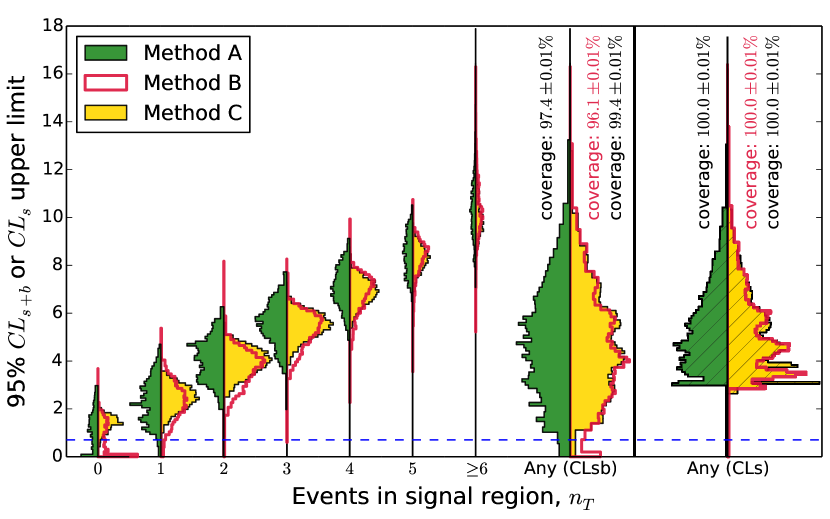
Figure 2: In the simple scenario described in the text (two leptons in two categories) computations using Method B are tractable. This figure therefore compares Methods A, B and C in that configuration. The 95% ${CL_{s+b}}$ and ${CL_{s}}$ upper limits on the rate of $T$ signal events for each of 19000 independent toy datasets are histogrammed. For each ‘column’, histograms are made for each of Methods A, B and C and plotted back-to-back; that is A is plotted opposite to B and C, which overlap. The ${CL_{s+b}}$ results are further divided into bins of observed $n_{T}$; in all cases the area of each histogram is proportional to the number of toy datasets used to create it. The dashed blue line indicates the true signal production rate, ${\nu_{{T}{R}}}=0.706$. The coverage of the observed limits of this truth rate are noted for the overall ${CL_{s+b}}$ and ${CL_{s}}$ results.

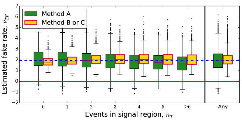
Figure 3: For the simple scenario described in the text (two leptons in two categories) in which computations using Method B remain tractable, the estimated fake rates for each of 19000 independent toy datasets are shown as a function of $n_{T}$, comparing Method A and Method B with box plots. The fake rate from Method C is by definition the same as that from Method B. The box plots indicate the median and lower & upper quartiles with the box, while the whiskers extend to most extreme datum within $1.5\times$inter-quartile range of the nearest quartile; this corresponds to the $k=1.5$ case as described in boxplots . Black dots are used to mark data points outside the range of the whiskers. The dashed blue line marks the true value of ${\nu_{{T}{F}}}=1.94$, and the red line delimits the unphysical ${\nu_{{T}{F}}}<0$ region.

3.2 Harder scenario – two leptons, eight categories

The simple scenario above has been extended to use eight categories instead of two. As per the parameterisation in Figure 1, this involves the addition of 24 extra parameters – twelve each for the signal and fake background from the addition of six $\beta$ and six $\pi$ terms. The full set of parameters can be found in Appendix B in Table 3. As before, 100 events were generated in each dataset, corresponding to a signal rate of 0.748 and a fake background rate of 2.77.

It was found that the increase in parameter space dimensionality was sufficient to increase the computation time for the likelihood maximisation to such an extent that producing limits with Method B became infeasible using the resources at the authors’ disposal; as such only results from Method A and Method C could be computed.

Figure 5 shows that the MLE fake rate for Method C is much more tightly constrained around the true value than the Method A estimate; moreover Method A gives even more significant deviations into negative values than with the simple scenario. Furthermore, as $n_{T}$ increases, the median fake rate from Method A decreases slightly, whereas that from Method C is stable for low event counts, only increasing slightly for larger $n_{T}$; the Method C behaviour seems more desirable here. Secondly, Figure 4 shows that the ${CL_{s+b}}$ limits derived in Method A suffer from under-coverage; the upper limit only bounds the true rate 92% of the time rather than the expected 95%. Finally the upper tails of the ${CL_{s+b}}$ limit are significantly more pronounced in Method A than in Method C, as can be seen when the limits are separated by $n_{T}$, as also included in Figure 4.

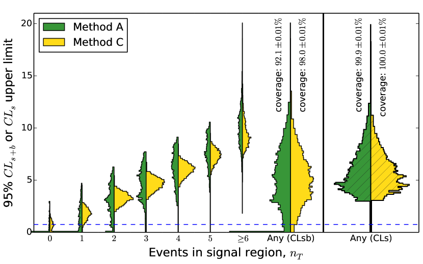
Figure 4: In the harder scenario described in the text (two leptons, eight categories) computations using Method B are no longer tractable. This figure therefore compares the only two usable Methods (A and C) in this more challenging case. The 95% ${CL_{s+b}}$ and ${CL_{s}}$ upper limits on the rate of $T$ signal events for each of 19000 independent toy datasets are histogrammed. For each ‘column’, histograms are made for each of Methods A and C and plotted back-to-back. The ${CL_{s+b}}$ results are further divided into bins of observed $n_{T}$; in all cases the area of each histogram is proportional to the number of toy datasets used to create it. The dashed blue line indicates the true signal production rate, ${\nu_{{T}{R}}}=0.748$. The coverage of the observed limits of this truth rate are noted for the overall ${CL_{s+b}}$ and ${CL_{s}}$ results.

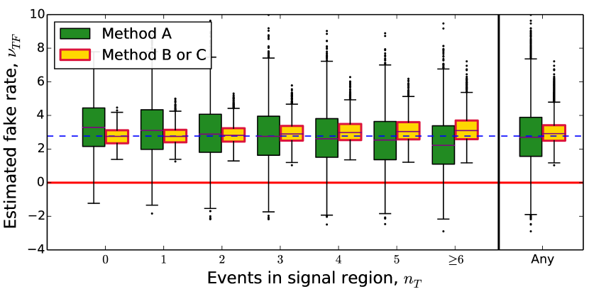
Figure 5: For the harder scenario described in the text (two leptons, eight categories) the fake rates estimated by Methods A and C for each of 19000 independent toy datasets are shown as a function of $n_{T}$ in the form of box plots, similarly to Figure 3. The dashed blue line marks the true value of ${\nu_{{T}{F}}}=2.77$, and the red line delimits the unphysical ${\nu_{{T}{F}}}<0$ region.

4 Conclusions

We have described the matrix method, used in many ATLAS and CMS analyses to estimate fake leptonic backgrounds, more completely than we have seen elsewhere. We have shown that it (Method A) produces a MLE fake rate under a restrictive set of conditions, but that these are rarely met in practice. We have shown that it has a number of undesired properties which result from its heuristic definition: (i) it can give physically meaningless results (predict negative fake rates), (ii) its fake rate estimates show an undesired bias as a function of the number of tight events in the signal region (as seen by the slope observed in the run of green boxes of Figures 3 and 5), and (iii) the limits it sets on fake rates are significantly more variable than those from better methods (as seen by the increased vertical extent of the Method A histograms in Figures 2 and 4 compared to those of Method B and Method C). We noted that, within the constraints of the frequentist profile-likelihood based framework considered, one cannot hope to constrain fake rates much better than Method B. However, we saw that the computational overheads of Method B precluded its use in all but the simplest of cases. Finally, we showed that it was possible to find a third approach, Method C, which is computationally of similar complexity to Method A and, though to some extent also heuristic in its definition, nonetheless reproduces much more closely the fake rate estimates of Method B. Method C, in contrast to the matrix method: (i) gives only physically meaningful results (predicts positive fake rates), (ii) its fake rate estimates are unbiased as a function of the number of tight events in the signal region (as seen by the lack of slope across the yellow boxes of Figures 3 and 5), and (iii) the limits it sets on fake rates are significantly less variable than those of Method A while being very close to those seen in the optimal Method B (again see Figures 2 and 4). The improvements seen in Method C over Method A are particularly notable in signal regions having few events.

A possible advantage of Method B and Method C not explored in this paper is afforded by their ability, if desired, to encapsulate background processes which can contribute by both real and fake events e.g. in different decay modes by use of different parameter trees. Further to this, it may be found that measurements in additional regions could constrain some of these parameters, much like the efficiencies are already constrained. Whilst speculative, further research in this area has the potential to provide even greater benefits over the original matrix method.

Appendix A Origin of matrix method approximation

It was stated earlier that, under appropriate conditions, $\hat{n}_{R}$ and $\hat{n}_{F}$ are maximum likelihood estimators for ${{\left<{n_{R}}\right>}}\equiv{\mathbb{E}\left[{{n_{R}}|{n_{T}},{n_{L}}}\right]}$ and ${{\left<{n_{F}}\right>}}\equiv{\mathbb{E}\left[{{n_{F}}|{n_{T}},{n_{L}}}\right]}$. This result, together with its limitations, is now presented.

A.1 Single lepton and single category

We shall firstly demonstrate this approximation in the simplified case with just a single lepton and category. The corresponding fully general derivation follows in the next section, but the logic it follows is largely the same.

When considering a likelihood as a product of Poisson terms as in equation (13), and neglecting the Gaussian terms involving the efficiencies, the negative log likelihood for the term arising from the background component will be

$${-\ln\mathcal{L}} =\sum_{\mathcal{T}\in\{T,L\}}\left({\nu_{\mathcal{T}}}-{n_{\mathcal{T}}}\ln{\nu_{\mathcal{T}}}\right).$$ (17)

Here we sum over two constraints, one from tight events and the other from loose. The means of Poisson distributions are denoted by $\nu_{\mathcal{T}}$. From equations (2) and (10), one finds

$${\nu_{\mathcal{T}}} =\sum_{\mathcal{R}\in\{R,F\}}\phi_{\mathcal{T}\mathcal{R}}{\nu_{\mathcal{R}}},$$ (18)

where $\nu_{\mathcal{R}}$ denotes the means of the Poisson distributions from which the numbers of real and fake events are drawn, and $\phi$ is the matrix of efficiencies with indices $\mathcal{T}$ and $\mathcal{R}$ referring to tight/loose and real/fake properties respectively.

One can now differentiate equation (17) with respect to ${\nu_{\mathcal{R}}},\forall\mathcal{R}\in\{R,F\}$, using the identity in equation (18), and find the MLE values for the rates, denoted $\nu_{\mathcal{T},\text{MLE}}$. In order to locate the minimum of the negative log likelihood, one sets these derivatives to 0, yielding

$$\sum_{\mathcal{T}\in\{T,L\}}\left(1-\frac{{n_{\mathcal{T}}}}{{\nu_{\mathcal{T},\text{MLE}}}}\right)\phi_{\mathcal{T}\mathcal{R}} =0,\quad\forall\mathcal{R}\in\{R,F\}.$$ (19)

These are satisfied if ${\nu_{\mathcal{T},\text{MLE}}}={n_{\mathcal{T}}}\ \forall\mathcal{T}\in\{T,L\}$, the result of which being that, upon inversion, equation (18) will look like

$${\nu_{\mathcal{R},\text{MLE}}}=\sum_{\mathcal{T}\in\{T,L\}}\phi^{-1}_{\mathcal{R}\mathcal{T}}{n_{\mathcal{T}}}={{\hat{n}}_{\mathcal{R}}{}},$$ (20)

analogously to equation (3).

Whilst this is a valid operation for the problem as stated above, it should be noted that the minimum of ${-\ln\mathcal{L}}$ is represented by equation (19) only when the components of ${\nu_{\mathcal{R},\text{MLE}}}$ are $>0$.

To conclude, equation (20) shows how the matrix method estimator ${\hat{n}}_{\mathcal{R}}{}$ is identical to the MLE values $\nu_{\mathcal{R},\text{MLE}}$ in the simplified single-lepton matrix method, if the condition above is met.

A.2 Multiple leptons and multiple categories

When considering a likelihood as a product of Poisson terms as in equation (13), and neglecting the Gaussian terms involving the efficiencies, the negative log likelihood for the term arising from the background component will be

$${-\ln\mathcal{L}} =\sum_{\bm{\omega},\bm{\beta}}\left({\nu_{\mathcal{T}}}^{\bm{\omega}}_{\bm{\beta}}-{n_{\mathcal{T}}}^{\bm{\omega}}_{\bm{\beta}}\ln{\nu_{\mathcal{T}}}^{\bm{\omega}}_{\bm{\beta}}\right),$$ (21)

where for a set of $m$ leptons the categories and tight/looseness information are compacted into vectors $\bm{\omega}$ and $\bm{\beta}$ of length $m$ respectively. Note also that the means of Poisson distributions are denoted in the general notation by e.g. $\nu_{\mathcal{T}}$. From equations (2) and (10), one finds

$${\nu_{\mathcal{T}}}^{\bm{\omega}}_{\bm{\beta}}=\sum_{\bm{\alpha^{\prime}}}{{\Phi_{\bm{\omega}}}_{\bm{\beta}}^{\ \bm{\alpha^{\prime}}}}{\nu_{\mathcal{R}}}^{\bm{\omega}}_{\bm{\alpha^{\prime}}},{{\Phi_{\bm{\omega}}}_{\bm{\beta}}^{\ \bm{\alpha^{\prime}}}}={{\phi_{\omega_{i_{1}}}}_{\beta_{1}}^{\ \alpha^{\prime}_{1}}}{{\phi_{\omega_{i_{2}}}}_{\beta_{2}}^{\ \alpha^{\prime}_{2}}}\ \cdots,$$ (22)

where $\bm{\alpha^{\prime}}$ is a vector representing whether each lepton is real or fake.

One can now differentiate equation (21) with respect to ${\nu_{\mathcal{R}}}^{\bm{\omega}}_{\bm{\alpha}},\ \forall\bm{\omega},\bm{\alpha}$, using the identity in equation (22), and find the MLE values for the rates, denoted e.g. $\nu_{\mathcal{T},\text{MLE}}$. In order to locate the minimum of the negative log likelihood, one sets all these derivatives to 0, yielding

$$\sum_{\bm{\beta^{\prime}}}\left(1-\frac{{n_{\mathcal{T}}}^{\bm{\omega}}_{\bm{\beta^{\prime}}}}{{\nu_{\mathcal{T},\text{MLE}}}^{\bm{\omega}}_{\bm{\beta^{\prime}}}}\right){{\Phi_{\bm{\omega}}}_{\bm{\alpha}}^{\ \bm{\beta^{\prime}}}} =0,\quad\forall\bm{\omega},\bm{\alpha}.$$ (23)

These are satisfied if ${\nu_{\mathcal{T},\text{MLE}}}^{\bm{\omega}}_{\bm{\beta^{\prime}}}={n_{\mathcal{T}}}^{\bm{\omega}}_{\bm{\beta^{\prime}}}\ \forall\bm{\beta^{\prime}}$, the result of which being that, upon inversion, equation (22) will look like

$${\nu_{\mathcal{R},\text{MLE}}}^{\bm{\omega}}_{\bm{\alpha}}=\sum_{\bm{\beta^{\prime}}}{{\Phi^{-1}_{\bm{\omega}}}_{\bm{\beta^{\prime}}}^{\ \bm{\alpha}}}{n_{\mathcal{T}}}^{\bm{\omega}}_{\bm{\beta^{\prime}}}={{\hat{n}}_{\mathcal{R}}{}}^{\bm{\omega}}_{\bm{\alpha}},$$ (24)

analogously to equation (3).

Whilst this is a valid operation for the problem as stated above, it should be noted that the minimum of ${-\ln\mathcal{L}}$ is represented by equation (23) only when the components of ${\nu_{\mathcal{R},\text{MLE}}}^{\bm{\omega}}_{\bm{\alpha}}$ are $>0$. Incidentally, is also only useful in the case where the components of ${\nu_{\mathcal{R},\text{MLE}}}^{\bm{\omega}}_{\bm{\alpha}}$ are readily assigned to either signal plus other ‘real’ backgrounds (those typically estimated from MC samples) and the fake background.

To conclude, equation (24) shows how the matrix method estimator ${\hat{n}}_{\mathcal{R}}{}$ is identical to the MLE values $\nu_{\mathcal{R},\text{MLE}}$ in the fully generalised matrix method, if the conditions above are met.

Appendix B Tables of parameters

Parameters used to configure the toy generator may be found in the following tables:

Object	Signal			Background
category	$\nu_{\tilde{L}}$	$\beta$	$\pi$	$\nu_{\tilde{L}}$	$\beta$	$\pi$	${\varepsilon_{r}}$	${\varepsilon_{f}}$
$\omega_{1}$	0.01	0.6	0	0.99	0.6	1	0.8	0.1
$\omega_{2}$	–	0.4	0	–	0.4	1	0.9	0.2

Table 2: Parameters controlling the simple scenario with exactly two leptons, and two categories for each lepton. The parameters are as described in Figure 1, however $\alpha_{2}=1$ and $\alpha_{i}=0\ \forall i\neq 2$. The overall production rate of events is $\nu_{\tilde{L}}$, each one of which is filtered through the decision tree. Components marked with a ‘–’ are not applicable in the context.

Object	Signal			Background
category	$\nu_{\tilde{L}}$	$\beta$	$\pi$	$\nu_{\tilde{L}}$	$\beta$	$\pi$	${\varepsilon_{r}}$	${\varepsilon_{f}}$
$\omega_{1}$	0.01	0.086	0	0.99	0.184	1	0.8	0.1
$\omega_{2}$	–	0.143	0	–	0.008	1	0.8	0.2
$\omega_{3}$	–	0.110	0	–	0.182	1	0.8	0.1
$\omega_{4}$	–	0.010	0	–	0.123	1	0.8	0.3
$\omega_{5}$	–	0.092	0	–	0.102	1	0.9	0.2
$\omega_{6}$	–	0.284	0	–	0.081	1	0.9	0.1
$\omega_{7}$	–	0.245	0	–	0.106	1	0.9	0.4
$\omega_{8}$	–	0.030	0	–	0.214	1	0.9	0.1

Table 3: Parameters controlling the simple scenario with exactly two leptons, and eight categories for each lepton. The parameters are as described in Figure 1, however $\alpha_{2}=1$ and $\alpha_{i}=0\ \forall i\neq 2$. The overall production rate of events is $\nu_{\tilde{L}}$, each one of which is filtered through the decision tree. Components marked with a ‘–’ are not applicable in the context.

References

- (1) ATLAS Collaboration, Search for strong production of supersymmetric particles in final states with missing transverse momentum and at least three b-jets using 20.1 fb−1 of pp collisions at sqrt(s) = 8 TeV with the ATLAS Detector., Tech. Rep. ATLAS-CONF-2013-061, CERN, Geneva, Jun, 2013.
- (2) ATLAS Collaboration, Background studies for top-pair production in lepton plus jets final states in ATLAS data, Tech. Rep. ATLAS-CONF-2010-087, CERN, Geneva, Oct, 2010.
- (3) ATLAS Collaboration, Search for supersymmetry using final states with one lepton, jets, and missing transverse momentum with the ATLAS detector in TeV , Phys.Rev.Lett. 106 (2011) 131802, [arXiv:1102.2357].
- (4) ATLAS Collaboration, Search for an excess of events with an identical flavour lepton pair and significant missing transverse momentum in TeV proton-proton collisions with the ATLAS detector, Eur.Phys.J. C71 (2011) 1647, [arXiv:1103.6208].
- (5) ATLAS Collaboration, Search for supersymmetric particles in events with lepton pairs and large missing transverse momentum in TeV proton-proton collisions with the ATLAS experiment, Eur.Phys.J. C71 (2011) 1682, [arXiv:1103.6214].
- (6) ATLAS Collaboration, Search for pair production of first or second generation leptoquarks in proton-proton collisions at TeV using the ATLAS detector at the LHC, Phys.Rev. D83 (2011) 112006, [arXiv:1104.4481].
- (7) ATLAS Collaboration, Measurement of the cross section for the production of a boson in association with jets in collisions at TeV with the ATLAS detector, Phys.Lett. B707 (2012) 418–437, [arXiv:1109.1470].
- (8) ATLAS Collaboration, Search for anomalous production of prompt like-sign muon pairs and constraints on physics beyond the Standard Model with the ATLAS detector, Phys.Rev. D85 (2012) 032004, [arXiv:1201.1091].
- (9) ATLAS Collaboration, Search for pair-produced heavy quarks decaying to Wq in the two-lepton channel at TeV with the ATLAS detector, Phys.Rev. D86 (2012) 012007, [arXiv:1202.3389].
- (10) ATLAS Collaboration, Observation of spin correlation in events from pp collisions at sqrt(s) = 7 TeV using the ATLAS detector, Phys.Rev.Lett. 108 (2012) 212001, [arXiv:1203.4081].
- (11) ATLAS Collaboration, A search for resonances with the ATLAS detector in 2.05 fb-1 of proton-proton collisions at TeV, Eur.Phys.J. C72 (2012) 2083, [arXiv:1205.5371].
- (12) ATLAS Collaboration, A search for resonances in lepton+jets events with highly boosted top quarks collected in collisions at TeV with the ATLAS detector, JHEP 1209 (2012) 041, [arXiv:1207.2409].
- (13) ATLAS Collaboration, ATLAS search for a heavy gauge boson decaying to a charged lepton and a neutrino in collisions at TeV, Eur.Phys.J. C72 (2012) 2241, [arXiv:1209.4446].
- (14) ATLAS Collaboration, Search for resonant top plus jet production in + jets events with the ATLAS detector in collisions at TeV, Phys.Rev. D86 (2012) 091103, [arXiv:1209.6593].
- (15) ATLAS Collaboration, Search for Supersymmetry in Events with Large Missing Transverse Momentum, Jets, and at Least One Tau Lepton in 7 TeV Proton-Proton Collision Data with the ATLAS Detector, Eur.Phys.J. C72 (2012) 2215, [arXiv:1210.1314].
- (16) ATLAS Collaboration, Measurement of production in collisions at TeV and limits on anomalous and couplings with the ATLAS detector, JHEP 1303 (2013) 128, [arXiv:1211.6096].
- (17) ATLAS Collaboration, Multi-channel search for squarks and gluinos in TeV collisions with the ATLAS detector, Eur.Phys.J. C73 (2013) 2362, [arXiv:1212.6149].
- (18) ATLAS Collaboration, Search for resonances in the lepton plus jets final state with ATLAS using 4.7 fb-1 of collisions at TeV, Phys.Rev. D88 (2013), no. 1 012004, [arXiv:1305.2756].
- (19) ATLAS Collaboration, Measurement of Top Quark Polarization in Top-Antitop Events from Proton-Proton Collisions at = 7 TeV Using the ATLAS Detector, Phys.Rev.Lett. 111 (2013), no. 23 232002, [arXiv:1307.6511].
- (20) ATLAS Collaboration, Measurement of the top quark pair production charge asymmetry in proton-proton collisions at = 7 TeV using the ATLAS detector, JHEP 1402 (2014) 107, [arXiv:1311.6724].
- (21) ATLAS Collaboration, Search for a Multi-Higgs Boson Cascade in events with the ATLAS detector in pp collisions at √s = 8 TeV, Phys.Rev. D89 (2014) 032002, [arXiv:1312.1956].
- (22) ATLAS Collaboration, Measurement of the production of a boson in association with a charm quark in collisions at 7 TeV with the ATLAS detector, JHEP 1405 (2014) 068, [arXiv:1402.6263].
- (23) ATLAS Collaboration, Search for direct top-squark pair production in final states with two leptons in pp collisions at 8TeV with the ATLAS detector, JHEP 1406 (2014) 124, [arXiv:1403.4853].
- (24) ATLAS Collaboration, Search for direct top squark pair production in events with a Z boson, b-jets and missing transverse momentum in =8 TeV pp collisions with the ATLAS detector, Eur.Phys.J. C74 (2014) 2883, [arXiv:1403.5222].
- (25) ATLAS Collaboration, Search for direct production of charginos, neutralinos and sleptons in final states with two leptons and missing transverse momentum in collisions at 8 TeV with the ATLAS detector, JHEP 1405 (2014) 071, [arXiv:1403.5294].
- (26) ATLAS Collaboration, Search for supersymmetry at =8 TeV in final states with jets and two same-sign leptons or three leptons with the ATLAS detector, JHEP 1406 (2014) 035, [arXiv:1404.2500].
- (27) ATLAS Collaboration, Search for microscopic black holes and string balls in final states with leptons and jets with the ATLAS detector at = 8 TeV, arXiv:1405.4254.
- (28) ATLAS Collaboration, Search for top squark pair production in final states with one isolated lepton, jets, and missing transverse momentum in 8 TeV pp collisions with the ATLAS detector, arXiv:1407.0583.
- (29) ATLAS Collaboration, Search for strong production of supersymmetric particles in final states with missing transverse momentum and at least three b-jets at 8 TeV proton-proton collisions with the ATLAS detector, arXiv:1407.0600.
- (30) ATLAS Collaboration, Search for supersymmetry in events with large missing transverse momentum, jets, and at least one tau lepton in 20 fb-1 of =8 TeV proton-proton collision data with the ATLAS detector, arXiv:1407.0603.
- (31) ATLAS Collaboration, Measurement of the production cross-section as a function of jet multiplicity and jet transverse momentum in 7 TeV proton-proton collisions with the ATLAS detector, arXiv:1407.0891.
- (32) CMS Collaboration, Measurement of the top-quark mass in events with dilepton final states in collisions at TeV, Eur.Phys.J. C72 (2012) 2202, [arXiv:1209.2393].
- (33) CMS Collaboration, Identification of b-quark jets with the CMS experiment, JINST 8 (2013) P04013, [arXiv:1211.4462].
- (34) CMS Collaboration, Search for a Higgs boson decaying into a b-quark pair and produced in association with b quarks in proton-proton collisions at 7 TeV, Phys.Lett. B722 (2013) 207–232, [arXiv:1302.2892].
- (35) CMS Collaboration, Measurement of the production cross section in the dilepton channel in collisions at TeV, JHEP 1211 (2012) 067, [arXiv:1208.2671].
- (36) B. Mistlberger and F. Dulat, Limit setting procedures and theoretical uncertainties in Higgs boson searches, arXiv:1204.3851.
- (37) BIPM, IEC, IFCC, ISO, IUPAC, IUPAP, and OIML, Guide to the Expression of Uncertainty in Measurement. International Organization for Standardization, 1995.
- (38) ATLAS Collaboration, K. Cranmer. private communication, 2013.
- (39) F. James and M. Roos, Minuit: A System for Function Minimization and Analysis of the Parameter Errors and Correlations, Comput.Phys.Commun. 10 (1975) 343–367.
- (40) G. Cowan, K. Cranmer, E. Gross, and O. Vitells, Asymptotic formulae for likelihood-based tests of new physics, European Physical Journal C 71 (Feb., 2011) 1554, [arXiv:1007.1727].
- (41) K. Cranmer, Frequentist Hypothesis Testing with Background Uncertainty, in Statistical Problems in Particle Physics, Astrophysics, and Cosmology (L. Lyons, R. Mount, and R. Reitmeyer, eds.), p. 261, 2003. physics/0310108.
- (42) M. Frigge, D. C. Hoaglin, and B. Iglewicz, Some implementations of the boxplot, The American Statistician 43 (1989), no. 1 pp. 50–54.