Scalable Kernel Methods via Doubly Stochastic Gradients

Bo Dai1 Bo Xie1 Niao He2 Yingyu Liang1 Anant Raj1 Maria-Florina Balcan3 Le Song1
1 College of Computing
Georgia Institute of Technology
{bodai
bxie33 yliang39 araj34}@gatech.edu lsong@cc.gatech.edu
2 School of Industrial & Systems Engineering
Georgia Institute of Technology
nhe6@gatech.edu
3 School of Computer Science
Carnegie Mellon University
ninamf@cs.cmu.edu
Abstract

The general perception is that kernel methods are not scalable, and neural nets are the methods of choice for large-scale nonlinear learning problems. Or have we simply not tried hard enough for kernel methods? Here we propose an approach that scales up kernel methods using a novel concept called β€œdoubly stochastic functional gradients”. Our approach relies on the fact that many kernel methods can be expressed as convex optimization problems, and we solve the problems by making two unbiased stochastic approximations to the functional gradient, one using random training points and another using random features associated with the kernel, and then descending using this noisy functional gradient. Our algorithm is simple, does not need to commit to a preset number of random features, and allows the flexibility of the function class to grow as we see more incoming data in the streaming setting. We show that a function learned by this procedure after t𝑑t iterations converges to the optimal function in the reproducing kernel Hilbert space in rate O​(1/t)𝑂1𝑑O(1/t), and achieves a generalization performance of O​(1/t)𝑂1𝑑O(1/\sqrt{t}). Our approach can readily scale kernel methods up to the regimes which are dominated by neural nets. We show that our method can achieve competitive performance to neural nets in datasets such as 2.3 million energy materials from MolecularSpace, 8 million handwritten digits from MNIST, and 1 million photos from ImageNet using convolution features.

1 Introduction

The general perception is that kernel methods are not scalable. When it comes to large-scale nonlinear learning problems, the methods of choice so far are neural nets where theoretical understanding remains incomplete. Are kernel methods really not scalable? Or is it simply because we have not tried hard enough, while neural nets have exploited sophisticated design of feature architectures, virtual example generation for dealing with invariance, stochastic gradient descent for efficient training, and GPUs for further speedup?

A bottleneck in scaling up kernel methods is the storage and computation of the kernel matrix, K𝐾K, which is usually dense. Storing the matrix requires O​(n2)𝑂superscript𝑛2O(n^{2}) space, and computing it takes O​(n2​d)𝑂superscript𝑛2𝑑O(n^{2}d) operations, where n𝑛n is the number of data points and d𝑑d is the dimension. There have been many great attempts to scale up kernel methods, including efforts from numerical linear algebra, functional analysis, and numerical optimization perspectives.

A common numerical linear algebra approach is to approximate the kernel matrix using low-rank factors, Kβ‰ˆAβŠ€β€‹A𝐾superscript𝐴top𝐴K\approx A^{\top}A, with Aβˆˆβ„rΓ—n𝐴superscriptβ„π‘Ÿπ‘›A\in\mathbb{R}^{r\times n} and rank rβ©½nπ‘Ÿπ‘›r\leqslant n. This low-rank approximation usually requires O​(n​r2+n​r​d)𝑂𝑛superscriptπ‘Ÿ2π‘›π‘Ÿπ‘‘O(nr^{2}+nrd) operations, and then subsequent kernel algorithms can directly operate on A𝐴A. Many works, such as Greedy basis selection techniquesΒ [1], NystrΓΆm approximationΒ [2] and incomplete Cholesky decompositionΒ [3], all followed this strategy. In practice, one observes that kernel methods with approximated kernel matrices often result in a few percentage of losses in performance. In fact, without further assumption on the regularity of the kernel matrix, the generalization ability after low-rank approximation is typically of the order O​(1/r+1/n)𝑂1π‘Ÿ1𝑛O(1/\sqrt{r}+1/\sqrt{n})Β [4, 5], which implies that the rank needs to be nearly linear in the number of data points! Thus, in order for kernel methods to achieve the best generalization ability, the low-rank approximation based approaches quickly become impractical for big datasets due to their O​(n3+n2​d)𝑂superscript𝑛3superscript𝑛2𝑑O(n^{3}+n^{2}d) preprocessing time and O​(n2)𝑂superscript𝑛2O(n^{2}) memory requirement.

Random feature approximation is another popular approach for scaling up kernel methodsΒ [6, 7]. Instead of approximating the kernel matrix, the method directly approximates the kernel function using explicit feature maps. The advantage of this approach is that the random feature matrix for n𝑛n data points can be computed in time O​(n​r​d)π‘‚π‘›π‘Ÿπ‘‘O(nrd) using O​(n​r)π‘‚π‘›π‘ŸO(nr) memory, where rπ‘Ÿr is the number of random features. Subsequent algorithms then only operate on an O​(n​r)π‘‚π‘›π‘ŸO(nr) matrix. Similar to low-rank kernel matrix approximation approach, the generalization ability of random feature approach is of the order O​(1/r+1/n)𝑂1π‘Ÿ1𝑛O(1/\sqrt{r}+1/\sqrt{n})Β [8, 9], which implies that the number of random features also needs to be O​(n)𝑂𝑛O(n). Another common drawback of these two approaches is that it is not easy to adapt the solution from a small rπ‘Ÿr to a large rβ€²superscriptπ‘Ÿβ€²r^{\prime}. Often one is interested in increasing the kernel matrix approximation rank or the number of random features to obtain a better generalization ability. Then special procedures need to be designed to reuse the solution obtained from a small rπ‘Ÿr, which is not straightforward.

Another approach that addresses the scalability issue rises from optimization perspective. One general strategy is to solve the dual forms of kernel methods using coordinate or block-coordinate descentΒ (e.g.,Β [10, 11, 12]). By doing so, each iteration of the algorithm only incurs O​(n​r​d)π‘‚π‘›π‘Ÿπ‘‘O(nrd) computation and O​(n​r)π‘‚π‘›π‘ŸO(nr) memory, where rπ‘Ÿr is the size of the parameter block. A second strategy is to perform functional gradient descent by looking at a batch of data points at a timeΒ (e.g.,Β [13, 15]). Thus, the computation and memory requirements are also O​(n​r​d)π‘‚π‘›π‘Ÿπ‘‘O(nrd) and O​(n​r)π‘‚π‘›π‘ŸO(nr) respectively in each iteration, where rπ‘Ÿr is the batch size. These approaches can easily change to a different rπ‘Ÿr without restarting the optimization and has no loss in generalization ability since they do not approximate the kernel matrix or function. However, a serious drawback of these approaches is that, without further approximation, all support vectors need to be kept for testing, which can be as big as the entire training set! (e.g., kernel ridge regression and non-separable nonlinear classification problems.)

In summary, there exists a delicate trade-off between computation, memory and statistics if one wants to scale up kernel methods. Inspired by various previous efforts, we propose a simple yet general strategy to scale up many kernel methods using a novel concept called β€œdoubly stochastic functional gradients”. Our method relies on the fact that most kernel methods can be expressed as convex optimization problems over functions in reproducing kernel Hilbert spaces (RKHS) and solved via functional gradient descent. Our algorithm proceeds by making two unbiased stochastic approximations to the functional gradient, one using random training points and the other one using random features associated with the kernel, and then descending using this noisy functional gradient. The key intuitions behind our algorithm originate from

  • (i)

    the property of stochastic gradient descent algorithm that as long as the stochastic gradient is unbiased, the convergence of the algorithm is guaranteedΒ [16]; and

  • (ii)

    the property of pseudo-random number generators that the random samples can in fact be completely determined by an initial value (a seed).

We exploit these properties and enable kernel methods to achieve better balances between computation, memory and statistics. Our method interestingly combines kernel methods, functional analysis, stochastic optimization and algorithmic trick, and it possesses a number of desiderata:

Generality and simplicity. Our approach applies to many kernel methods, such as kernel ridge regression, support vector machines, logistic regression, two-sample test, and many different types of kernels, such as shift-invariant kernels, polynomial kernels, general inner product kernels, and so on. The algorithm can be summarized in just a few lines of code (Algorithm 1 and 2). For a different problem and kernel, we just need to adapt the loss function and the random feature generator.

Flexibility. Different from previous uses of random features which typically prefix the number of features and then optimize over the feature weightings, our approach allows the number of random features, and hence the flexibility of the function class, to grow with the number of data points. This allows our method to be applicable to data streaming setting, which is not possible for previous random feature approach, and achieve the full potential of nonparametric methods.

Efficient computation. The key computation of our method is evaluating the doubly stochastic functional gradient, which involves the generation of the random features with specific random seeds and the evaluation of these random features on the small batch of data points. For iteration t𝑑t, the computational complexity is O​(t​d)𝑂𝑑𝑑O(td).

Small memory. The doubly stochasticity also allows us to avoid keeping the support vectors which becomes prohibitive in large-scale streaming setting. Instead, we just need to keep a small program for regenerating the random features, and sample previously used random feature according to pre-specified random seeds. For iteration t𝑑t, the memory needed is O​(t)𝑂𝑑O(t) independent of the dimension of the data.

Theoretical guarantees. We provide a novel and nontrivial analysis involving Hilbert space martingale and a newly proved recurrence relation, and show that the estimator produced by our algorithm, which might be outside of the RKHS, converges to the optimal RKHS function. More specifically, both in expectation and with high probability, our algorithm can estimate the optimal function in the RKHS in the rate of O​(1/t)𝑂1𝑑O(1/t), which are indeed optimalΒ [16], and achieve a generalization bound of O​(1/t)𝑂1𝑑O(1/\sqrt{t}). The variance of the random features, introduced during our second approximation to the functional gradient, only contributes additively to the constant in the final convergence rate. These results are the first of the kind in kernel method literature, which can be of independent interest.

Strong empirical performance. Our algorithm can readily scale kernel methods up to the regimes which are previously dominated by neural nets. We show that our method compares favorably to other scalable kernel methods in medium scale datasets, and to neural nets in big datasets such as 8 million handwritten digits from MNIST, 2.3 million materials from MolecularSpace, and 1 million photos from ImageNet using convolution features. Our results suggest that kernel methods, theoretically well-grounded methods, can potentially replace neural nets in many large scale real-world problems where nonparametric estimation are needed.

In the remainder, we will first introduce preliminaries on kernel methods and functional gradients. We will then describe our algorithm and provide both theoretical and empirical supports.

2 Duality between Kernels and Random Processes

Kernel methods owe their name to the use of kernel functions, k​(x,xβ€²):𝒳×𝒳↦ℝ:π‘˜π‘₯superscriptπ‘₯β€²maps-to𝒳𝒳ℝk(x,x^{\prime}):\mathcal{X}\times\mathcal{X}\mapsto\mathbb{R}, which are symmetric positive definite (PD), meaning that for all n>1𝑛1n>1, and x1,…,xnβˆˆπ’³subscriptπ‘₯1…subscriptπ‘₯𝑛𝒳x_{1},\ldots,x_{n}\in\mathcal{X}, and c1,…,cnβˆˆβ„subscript𝑐1…subscript𝑐𝑛ℝc_{1},\ldots,c_{n}\in\mathbb{R}, we have βˆ‘i,j=1nci​cj​k​(xi,xj)β©Ύ0superscriptsubscript𝑖𝑗1𝑛subscript𝑐𝑖subscriptπ‘π‘—π‘˜subscriptπ‘₯𝑖subscriptπ‘₯𝑗0\sum_{i,j=1}^{n}c_{i}c_{j}k(x_{i},x_{j})\geqslant 0. There is an intriguing duality between kernels and stochastic processes which will play a crucial role in our later algorithm design. More specifically,

Theorem 1 (e.g.,[17]; [18])

If k​(x,xβ€²)π‘˜π‘₯superscriptπ‘₯β€²k(x,x^{\prime}) is a PD kernel, then there exists a set ΩΩ\Omega, a measure β„™β„™\mathbb{P} on ΩΩ\Omega, and random feature ϕω​(x):𝒳↦ℝ:subscriptitalic-Ο•πœ”π‘₯maps-to𝒳ℝ\phi_{\omega}(x):\mathcal{X}\mapsto\mathbb{R} from L2​(Ξ©,β„™)subscript𝐿2Ξ©β„™L_{2}(\Omega,\mathbb{P}), such that k​(x,xβ€²)=βˆ«Ξ©Ο•Ο‰β€‹(x)​ϕω​(xβ€²)​𝑑ℙ​(Ο‰).π‘˜π‘₯superscriptπ‘₯β€²subscriptΞ©subscriptitalic-Ο•πœ”π‘₯subscriptitalic-Ο•πœ”superscriptπ‘₯β€²differential-dβ„™πœ”k(x,x^{\prime})=\int_{\Omega}\,\phi_{\omega}(x)\,\phi_{\omega}(x^{\prime})\,d\mathbb{P}(\omega).

Essentially, the above integral representation relates the kernel function to a random process Ο‰πœ”\omega with measure ℙ​(Ο‰)β„™πœ”\mathbb{P}(\omega). Note that the integral representation may not be unique. For instance, the random process can be a Gaussian process on 𝒳𝒳\mathcal{X} with the sample function ϕω​(x)subscriptitalic-Ο•πœ”π‘₯\phi_{\omega}(x), and k​(x,xβ€²)π‘˜π‘₯superscriptπ‘₯β€²k(x,x^{\prime}) is simply the covariance function between two point xπ‘₯x and xβ€²superscriptπ‘₯β€²x^{\prime}. If the kernel is also continuous and shift invariant,Β i.e.,Β k​(x,xβ€²)=k​(xβˆ’xβ€²)π‘˜π‘₯superscriptπ‘₯β€²π‘˜π‘₯superscriptπ‘₯β€²k(x,x^{\prime})=k(x-x^{\prime}) for xβˆˆβ„dπ‘₯superscriptℝ𝑑x\in\mathbb{R}^{d}, then the integral representation specializes into a form characterized by inverse Fourier transformation (e.g.,Β [19, Theorem 6.6]),

Theorem 2 (Bochner)

A continuous, real-valued, symmetric and shift-invariant function k​(xβˆ’xβ€²)π‘˜π‘₯superscriptπ‘₯β€²k(x-x^{\prime}) on ℝdsuperscriptℝ𝑑\mathbb{R}^{d} is a PD kernel if and only if there is a finite non-negative measure ℙ​(Ο‰)β„™πœ”\mathbb{P}(\omega) on ℝdsuperscriptℝ𝑑\mathbb{R}^{d}, such that k​(xβˆ’xβ€²)=βˆ«β„deiβ€‹Ο‰βŠ€β€‹(xβˆ’xβ€²)​𝑑ℙ​(Ο‰)=βˆ«β„dΓ—[0,2​π]2​cos⁑(Ο‰βŠ€β€‹x+b)​cos⁑(Ο‰βŠ€β€‹xβ€²+b)​d​(ℙ​(Ο‰)×ℙ​(b)),π‘˜π‘₯superscriptπ‘₯β€²subscriptsuperscriptℝ𝑑superscript𝑒𝑖superscriptπœ”topπ‘₯superscriptπ‘₯β€²differential-dβ„™πœ”subscriptsuperscriptℝ𝑑02πœ‹2superscriptπœ”topπ‘₯𝑏superscriptπœ”topsuperscriptπ‘₯β€²π‘π‘‘β„™πœ”β„™π‘k(x-x^{\prime})=\int_{\mathbb{R}^{d}}\,e^{i\omega^{\top}(x-x^{\prime})}\,d\mathbb{P}(\omega)=\int_{\mathbb{R}^{d}\times[0,2\pi]}2\,\cos(\omega^{\top}x+b)\,\cos(\omega^{\top}x^{\prime}+b)\,d\left(\mathbb{P}(\omega)\times\mathbb{P}(b)\right), where ℙ​(b)ℙ𝑏\mathbb{P}(b) is a uniform distribution on [0,2​π]02πœ‹[0,2\pi], and ϕω​(x)=2​cos⁑(Ο‰βŠ€β€‹x+b)subscriptitalic-Ο•πœ”π‘₯2superscriptπœ”topπ‘₯𝑏\phi_{\omega}(x)=\sqrt{2}\cos(\omega^{\top}x+b).

For Gaussian RBF kernel, k​(xβˆ’xβ€²)=exp⁑(βˆ’β€–xβˆ’xβ€²β€–2/2​σ2)π‘˜π‘₯superscriptπ‘₯β€²superscriptnormπ‘₯superscriptπ‘₯β€²22superscript𝜎2k(x-x^{\prime})=\exp(-\|x-x^{\prime}\|^{2}/2\sigma^{2}), this yields a Gaussian distribution ℙ​(Ο‰)β„™πœ”\mathbb{P}(\omega) with density proportional to exp⁑(βˆ’Οƒ2​‖ω‖2/2)superscript𝜎2superscriptnormπœ”22\exp(-\sigma^{2}\|\omega\|^{2}/2); for the Laplace kernel, this yields a Cauchy distribution; and for the Martern kernel, this yields the convolutions of the unit ballΒ [20].

Similar representation where the explicit form of ϕω​(x)subscriptitalic-Ο•πœ”π‘₯\phi_{\omega}(x) and ℙ​(Ο‰)β„™πœ”\mathbb{P}(\omega) are known can also be derived for rotation invariant kernel, k​(x,xβ€²)=k​(⟨x,xβ€²βŸ©)π‘˜π‘₯superscriptπ‘₯β€²π‘˜π‘₯superscriptπ‘₯β€²k(x,x^{\prime})=k(\left\langle x,x^{\prime}\right\rangle), using Fourier transformation on sphereΒ [20]. For polynomial kernels, k​(x,xβ€²)=(⟨x,xβ€²βŸ©+c)pπ‘˜π‘₯superscriptπ‘₯β€²superscriptπ‘₯superscriptπ‘₯′𝑐𝑝k(x,x^{\prime})=(\left\langle x,x^{\prime}\right\rangle+c)^{p}, a random tensor sketching approach can also be usedΒ [21]. Explicit random features have been designed for many other kernels, such as dot product kernelΒ [33], additive/multiplicative class of homogeneous kernelsΒ [34], e.g., Hellinger’s, Ο‡2superscriptπœ’2\chi^{2}, Jensen-Shannon’s and Intersection kernel, as well as kernels on Abelian semigroupsΒ [35]. We summarized these kernels with their explicit features and associated densities in TableΒ 1.

Table 1: Summary of kernels inΒ [6, 46, 33, 21, 34, 35, 45] and their explicit features
Kernel k​(x,xβ€²)π‘˜π‘₯superscriptπ‘₯β€²k(x,x^{\prime}) ϕω​(x)subscriptitalic-Ο•πœ”π‘₯\phi_{\omega}(x) p​(Ο‰)π‘πœ”p(\omega)
Gaussian exp⁑(βˆ’β€–xβˆ’xβ€²β€–222)superscriptsubscriptnormπ‘₯superscriptπ‘₯β€²222\exp(-\frac{\|x-x^{\prime}\|_{2}^{2}}{2}) exp⁑(βˆ’iβ€‹Ο‰βŠ€β€‹x)𝑖superscriptπœ”topπ‘₯\exp(-i\omega^{\top}x) (2​π)βˆ’d2​exp⁑(βˆ’β€–Ο‰β€–222)superscript2πœ‹π‘‘2superscriptsubscriptnormπœ”222{(2\pi)}^{-\frac{d}{2}}\exp(-\frac{\|\omega\|_{2}^{2}}{2})
Laplacian exp⁑(βˆ’β€–xβˆ’xβ€²β€–1)subscriptnormπ‘₯superscriptπ‘₯β€²1\exp(-{\|x-x^{\prime}\|_{1}}) exp⁑(βˆ’iβ€‹Ο‰βŠ€β€‹x)𝑖superscriptπœ”topπ‘₯\exp(-i\omega^{\top}x) ∏i=1d1π​(1+Ο‰i2)superscriptsubscriptproduct𝑖1𝑑1πœ‹1superscriptsubscriptπœ”π‘–2\prod_{i=1}^{d}\frac{1}{\pi(1+\omega_{i}^{2})}
Cauchy ∏i=1d21+(xiβˆ’xiβ€²)2superscriptsubscriptproduct𝑖1𝑑21superscriptsubscriptπ‘₯𝑖subscriptsuperscriptπ‘₯′𝑖2\prod_{i=1}^{d}\frac{2}{1+(x_{i}-x^{\prime}_{i})^{2}} exp⁑(βˆ’iβ€‹Ο‰βŠ€β€‹x)𝑖superscriptπœ”topπ‘₯\exp(-i\omega^{\top}x) exp⁑(βˆ’β€–Ο‰β€–1)subscriptnormπœ”1\exp(-{\|\omega\|_{1}})
MatΓ©rn 21βˆ’Ξ½Ξ“β€‹(Ξ½)​(2​ν​‖xβˆ’xβ€²β€–2β„“)ν​Kν​(2​ν​‖xβˆ’xβ€²β€–2β„“)superscript21πœˆΞ“πœˆsuperscript2𝜈subscriptnormπ‘₯superscriptπ‘₯β€²2β„“πœˆsubscript𝐾𝜈2𝜈subscriptnormπ‘₯superscriptπ‘₯β€²2β„“\frac{2^{1-\nu}}{\Gamma(\nu)}\bigg{(}\frac{\sqrt{2\nu}\|x-x^{\prime}\|_{2}}{\ell}\bigg{)}^{\nu}K_{\nu}\bigg{(}\frac{\sqrt{2\nu}\|x-x^{\prime}\|_{2}}{\ell}\bigg{)} exp⁑(βˆ’iβ€‹Ο‰βŠ€β€‹x)𝑖superscriptπœ”topπ‘₯\exp(-i\omega^{\top}x) h​(Ξ½,d,β„“)​(2​νℓ2+4​π2​‖ω‖22)Ξ½+d/2β„Žπœˆπ‘‘β„“superscript2𝜈superscriptβ„“24superscriptπœ‹2superscriptsubscriptnormπœ”22πœˆπ‘‘2h(\nu,d,\ell)\bigg{(}\frac{2\nu}{\ell^{2}}+4\pi^{2}\|\omega\|_{2}^{2}\bigg{)}^{\nu+d/2}
Dot Product βˆ‘n=0∞anβ€‹βŸ¨x,xβ€²βŸ©nanβ©Ύ0superscriptsubscript𝑛0subscriptπ‘Žπ‘›superscriptπ‘₯superscriptπ‘₯′𝑛subscriptπ‘Žπ‘›0\sum_{n=0}^{\infty}a_{n}\langle x,x^{\prime}\rangle^{n}\quad a_{n}\geqslant 0 aN​pN+1β€‹βˆi=1NΟ‰iβŠ€β€‹xsubscriptπ‘Žπ‘superscript𝑝𝑁1superscriptsubscriptproduct𝑖1𝑁superscriptsubscriptπœ”π‘–topπ‘₯\sqrt{a_{N}p^{N+1}}\prod_{i=1}^{N}\omega_{i}^{\top}x ℙ​[N=n]=1pn+1β„™delimited-[]𝑁𝑛1superscript𝑝𝑛1\mathbb{P}[N=n]=\frac{1}{p^{n+1}}
p​(Ο‰ij|N=n)=12Ο‰ij+12​121βˆ’Ο‰ij2𝑝conditionalsubscriptsuperscriptπœ”π‘—π‘–π‘π‘›superscript12subscriptsuperscriptπœ”π‘—π‘–12superscript121subscriptsuperscriptπœ”π‘—π‘–2p(\omega^{j}_{i}|N=n)=\frac{1}{2}^{\frac{\omega^{j}_{i}+1}{2}}\frac{1}{2}^{\frac{1-\omega^{j}_{i}}{2}}
Polynomial (⟨x,xβ€²βŸ©+c)psuperscriptπ‘₯superscriptπ‘₯′𝑐𝑝(\langle x,x^{\prime}\rangle+c)^{p} π™΅π™΅πšƒβˆ’1​(π™΅π™΅πšƒβ€‹(C1​x)βŠ™β€¦βŠ™π™΅π™΅πšƒβ€‹(Cp​x))superscriptπ™΅π™΅πšƒ1direct-productπ™΅π™΅πšƒsubscript𝐢1π‘₯β€¦π™΅π™΅πšƒsubscript𝐢𝑝π‘₯\mathtt{FFT}^{-1}(\mathtt{FFT}(C_{1}x)\odot\ldots\odot\mathtt{FFT}(C_{p}x)) Cj=Sj​Djsubscript𝐢𝑗subscript𝑆𝑗subscript𝐷𝑗C_{j}=S_{j}D_{j}
Djβˆˆβ„dΓ—d​Sjβˆˆβ„DΓ—dsubscript𝐷𝑗superscriptℝ𝑑𝑑subscript𝑆𝑗superscriptℝ𝐷𝑑D_{j}\in\mathbb{R}^{d\times d}\,S_{j}\in\mathbb{R}^{D\times d}
Hellinger βˆ‘i=1dxi​xiβ€²superscriptsubscript𝑖1𝑑subscriptπ‘₯𝑖subscriptsuperscriptπ‘₯′𝑖\sum_{i=1}^{d}\sqrt{x_{i}x^{\prime}_{i}} 2β€‹Ο‰βŠ€β€‹x2superscriptπœ”topπ‘₯2\omega^{\top}\sqrt{x} 12Ο‰i+12​121βˆ’Ο‰i2,Ο‰i∈{βˆ’1,+1}superscript12subscriptπœ”π‘–12superscript121subscriptπœ”π‘–2subscriptπœ”π‘–11\frac{1}{2}^{\frac{\omega_{i}+1}{2}}\frac{1}{2}^{\frac{1-\omega_{i}}{2}},\,\,\omega_{i}\in\{-1,+1\}
Ο‡2superscriptπœ’2\chi^{2} 2β€‹βˆ‘i=1dxi​xiβ€²xi+xiβ€²2superscriptsubscript𝑖1𝑑subscriptπ‘₯𝑖superscriptsubscriptπ‘₯𝑖′subscriptπ‘₯𝑖subscriptsuperscriptπ‘₯′𝑖2\sum_{i=1}^{d}\frac{x_{i}x_{i}^{\prime}}{x_{i}+x^{\prime}_{i}} [exp⁑(βˆ’i​ω​log⁑xj)​xj]j=1dsuperscriptsubscriptdelimited-[]π‘–πœ”subscriptπ‘₯𝑗subscriptπ‘₯𝑗𝑗1𝑑\big{[}\exp(-i\omega\log x_{j})\sqrt{x_{j}}\big{]}_{j=1}^{d} s​e​c​h​(π​ω)π‘ π‘’π‘β„Žπœ‹πœ”sech(\pi\omega)
Intersection βˆ‘i=1dmin⁑(xi,xiβ€²)superscriptsubscript𝑖1𝑑subscriptπ‘₯𝑖superscriptsubscriptπ‘₯𝑖′\sum_{i=1}^{d}\min(x_{i},x_{i}^{\prime}) [exp⁑(βˆ’i​ω​log⁑xj)​2​xj]j=1dsuperscriptsubscriptdelimited-[]π‘–πœ”subscriptπ‘₯𝑗2subscriptπ‘₯𝑗𝑗1𝑑\big{[}\exp(-i\omega\log x_{j})\sqrt{2x_{j}}\big{]}_{j=1}^{d} 1π​(1+4​ω2)1πœ‹14superscriptπœ”2\frac{1}{\pi(1+4\omega^{2})}
Jensen-Shannon βˆ‘i=1dKJ​S​(xi,xiβ€²)superscriptsubscript𝑖1𝑑subscript𝐾𝐽𝑆subscriptπ‘₯𝑖subscriptsuperscriptπ‘₯′𝑖\sum_{i=1}^{d}K_{JS}(x_{i},x^{\prime}_{i}) [exp⁑(βˆ’i​ω​log⁑xj)​2​xj]j=1dsuperscriptsubscriptdelimited-[]π‘–πœ”subscriptπ‘₯𝑗2subscriptπ‘₯𝑗𝑗1𝑑\big{[}\exp(-i\omega\log x_{j})\sqrt{2x_{j}}\big{]}_{j=1}^{d} s​e​c​h​(π​ω)log⁑4​(1+4​ω2)π‘ π‘’π‘β„Žπœ‹πœ”414superscriptπœ”2\frac{sech(\pi\omega)}{\log 4(1+4\omega^{2})}
Skewed-Ο‡2superscriptπœ’2\chi^{2} 2β€‹βˆi=1dxi+c​xiβ€²+cxi+xiβ€²+2​c2superscriptsubscriptproduct𝑖1𝑑subscriptπ‘₯𝑖𝑐subscriptsuperscriptπ‘₯′𝑖𝑐subscriptπ‘₯𝑖subscriptsuperscriptπ‘₯′𝑖2𝑐2\prod_{i=1}^{d}\frac{\sqrt{x_{i}+c}\sqrt{x^{\prime}_{i}+c}}{x_{i}+x^{\prime}_{i}+2c} exp⁑(βˆ’iβ€‹Ο‰βŠ€β€‹log⁑(x+c))𝑖superscriptπœ”topπ‘₯𝑐\exp(-i\omega^{\top}\log(x+c)) ∏i=1ds​e​c​h​(π​ωi)superscriptsubscriptproduct𝑖1π‘‘π‘ π‘’π‘β„Žπœ‹subscriptπœ”π‘–\prod_{i=1}^{d}sech(\pi\omega_{i})
Skewed-Intersection ∏i=1dmin⁑(xi+cxiβ€²+c,xiβ€²+cxi+c)superscriptsubscriptproduct𝑖1𝑑subscriptπ‘₯𝑖𝑐subscriptsuperscriptπ‘₯′𝑖𝑐subscriptsuperscriptπ‘₯′𝑖𝑐subscriptπ‘₯𝑖𝑐\prod_{i=1}^{d}\min\bigg{(}\sqrt{\frac{x_{i}+c}{x^{\prime}_{i}+c}},\sqrt{\frac{x^{\prime}_{i}+c}{x_{i}+c}}\bigg{)} exp⁑(βˆ’iβ€‹Ο‰βŠ€β€‹log⁑(x+c))𝑖superscriptπœ”topπ‘₯𝑐\exp(-i\omega^{\top}\log(x+c)) ∏i=1d1π​(1+4​ωi2)superscriptsubscriptproduct𝑖1𝑑1πœ‹14superscriptsubscriptπœ”π‘–2\prod_{i=1}^{d}\frac{1}{\pi(1+4\omega_{i}^{2})}
Exponential-Semigroup exp⁑(βˆ’Ξ²β€‹βˆ‘i=1dxi+xjβ€²)𝛽superscriptsubscript𝑖1𝑑subscriptπ‘₯𝑖subscriptsuperscriptπ‘₯′𝑗\exp(-\beta\sum_{i=1}^{d}\sqrt{x_{i}+x^{\prime}_{j}}) exp⁑(βˆ’Ο‰βŠ€β€‹x)superscriptπœ”topπ‘₯\exp(-\omega^{\top}x) ∏i=1dΞ²2​π​ωiβˆ’32​exp⁑(βˆ’Ξ²4​ωi)superscriptsubscriptproduct𝑖1𝑑𝛽2πœ‹superscriptsubscriptπœ”π‘–32𝛽4subscriptπœ”π‘–\prod_{i=1}^{d}\frac{\beta}{2\sqrt{\pi}}\omega_{i}^{-\frac{3}{2}}\exp(-\frac{\beta}{4\omega_{i}})
Reciprocal-Semigroup ∏i=1dΞ»xi+xiβ€²+Ξ»superscriptsubscriptproduct𝑖1π‘‘πœ†subscriptπ‘₯𝑖subscriptsuperscriptπ‘₯β€²π‘–πœ†\prod_{i=1}^{d}\frac{\lambda}{x_{i}+x^{\prime}_{i}+\lambda} exp⁑(βˆ’Ο‰βŠ€β€‹x)superscriptπœ”topπ‘₯\exp(-\omega^{\top}x) ∏i=1dλ​exp⁑(βˆ’Ξ»β€‹Ο‰i)superscriptsubscriptproduct𝑖1π‘‘πœ†πœ†subscriptπœ”π‘–\prod_{i=1}^{d}\lambda\exp(-\lambda\omega_{i})
Arc-Cosine 1π​‖xβ€–n​‖xβ€²β€–n​Jn​(ΞΈ)1πœ‹superscriptnormπ‘₯𝑛superscriptnormsuperscriptπ‘₯′𝑛subscriptπ½π‘›πœƒ\frac{1}{\pi}\|x\|^{n}\|x^{\prime}\|^{n}J_{n}(\theta) (Ο‰βŠ€β€‹x)n​max⁑(0,Ο‰βŠ€β€‹x)superscriptsuperscriptπœ”topπ‘₯𝑛0superscriptπœ”topπ‘₯(\omega^{\top}x)^{n}\max(0,\omega^{\top}x) 2β€‹Ο€βˆ’d2​exp⁑(βˆ’β€–Ο‰β€–222)2superscriptπœ‹π‘‘2superscriptsubscriptnormπœ”222{2\pi}^{-\frac{d}{2}}\exp(-\frac{\|\omega\|_{2}^{2}}{2})

Djsubscript𝐷𝑗D_{j} is random {Β±1}plus-or-minus1\{\pm 1\} diagonal matrix and the columns of Sjsubscript𝑆𝑗S_{j} are uniformly selected from {e1,…,eD}subscript𝑒1…subscript𝑒𝐷\{e_{1},\ldots,e_{D}\}. ν𝜈\nu and β„“β„“\ell are positive parameters.
h​(Ξ½,d,β„“)=2d​πd/2​Γ​(Ξ½+d/2)​(2​ν)νΓ​(Ξ½)​ℓ2β€‹Ξ½β„Žπœˆπ‘‘β„“superscript2𝑑superscriptπœ‹π‘‘2Ξ“πœˆπ‘‘2superscript2πœˆπœˆΞ“πœˆsuperscriptβ„“2𝜈h(\nu,d,\ell)=\frac{2^{d}\pi^{d/2}\Gamma(\nu+d/2)(2\nu)^{\nu}}{\Gamma(\nu)\ell^{2\nu}}. KΞ½subscript𝐾𝜈K_{\nu} is a modified Bessel function. KJ​S​(x,xβ€²)=x2​log2⁑x+xβ€²x+xβ€²2​log2⁑x+xβ€²xβ€²subscript𝐾𝐽𝑆π‘₯superscriptπ‘₯β€²π‘₯2subscript2π‘₯superscriptπ‘₯β€²π‘₯superscriptπ‘₯β€²2subscript2π‘₯superscriptπ‘₯β€²superscriptπ‘₯β€²K_{JS}(x,x^{\prime})=\frac{x}{2}\log_{2}\frac{x+x^{\prime}}{x}+\frac{x^{\prime}}{2}\log_{2}\frac{x+x^{\prime}}{x^{\prime}}.
ΞΈ=cosβˆ’1⁑xβŠ€β€‹xβ€²β€–x‖​‖xβ€²β€–πœƒsuperscript1superscriptπ‘₯topsuperscriptπ‘₯β€²normπ‘₯normsuperscriptπ‘₯β€²\theta=\cos^{-1}\frac{x^{\top}x^{\prime}}{\|x\|\|x^{\prime}\|}, Jn​(ΞΈ)=(βˆ’1)n​(sin⁑θ)2​n+1​(1sinβ‘ΞΈβ€‹βˆ‚βˆ‚ΞΈ)n​(Ο€βˆ’ΞΈsin⁑θ)subscriptπ½π‘›πœƒsuperscript1𝑛superscriptπœƒ2𝑛1superscript1πœƒπœƒπ‘›πœ‹πœƒπœƒJ_{n}(\theta)=(-1)^{n}(\sin\theta)^{2n+1}\bigg{(}\frac{1}{\sin\theta}\frac{\partial}{\partial\theta}\bigg{)}^{n}\bigg{(}\frac{\pi-\theta}{\sin\theta}\bigg{)}

Instead of finding the random process ℙ​(Ο‰)β„™πœ”\mathbb{P}(\omega) and function ϕω​(x)subscriptitalic-Ο•πœ”π‘₯\phi_{\omega}(x) given a kernel, one can go the reverse direction, and construct kernels from random processes and functions (e.g., [19]).

Theorem 3

If k​(x,xβ€²)=βˆ«Ξ©Ο•Ο‰β€‹(x)βŠ€β€‹Ο•Ο‰β€‹(xβ€²)​𝑑ℙ​(Ο‰)π‘˜π‘₯superscriptπ‘₯β€²subscriptΞ©subscriptitalic-Ο•πœ”superscriptπ‘₯topsubscriptitalic-Ο•πœ”superscriptπ‘₯β€²differential-dβ„™πœ”k(x,x^{\prime})=\int_{\Omega}\phi_{\omega}(x)^{\top}\phi_{\omega}(x^{\prime})\,d\mathbb{P}(\omega) for a nonnegative measure ℙ​(Ο‰)β„™πœ”\mathbb{P}(\omega) on ΩΩ\Omega and ϕω​(x):𝒳↦ℝr:subscriptitalic-Ο•πœ”π‘₯maps-to𝒳superscriptβ„π‘Ÿ\phi_{\omega}(x):\mathcal{X}\mapsto\mathbb{R}^{r}, each component from L2​(Ξ©,β„™)subscript𝐿2Ξ©β„™L_{2}(\Omega,\mathbb{P}), then k​(x,xβ€²)π‘˜π‘₯superscriptπ‘₯β€²k(x,x^{\prime}) is a PD kernel.

For instance, ϕω​(x):=cos⁑(Ο‰βŠ€β€‹ΟˆΞΈβ€‹(x)+b)assignsubscriptitalic-Ο•πœ”π‘₯superscriptπœ”topsubscriptπœ“πœƒπ‘₯𝑏\phi_{\omega}(x):=\cos(\omega^{\top}\psi_{\theta}(x)+b), where ΟˆΞΈβ€‹(x)subscriptπœ“πœƒπ‘₯\psi_{\theta}(x) can be a random convolution of the input xπ‘₯x parametrized by ΞΈπœƒ\theta, or ϕω​(x)=[ϕω1​(x),ϕω2​(x),…,ϕωr​(x)]subscriptitalic-Ο•πœ”π‘₯subscriptitalic-Ο•subscriptπœ”1π‘₯subscriptitalic-Ο•subscriptπœ”2π‘₯…subscriptitalic-Ο•subscriptπœ”π‘Ÿπ‘₯\phi_{\omega}(x)=[\phi_{\omega_{1}}(x),\phi_{\omega_{2}}(x),\ldots,\phi_{\omega_{r}}(x)], where ϕω1​(x)subscriptitalic-Ο•subscriptπœ”1π‘₯\phi_{\omega_{1}}(x) denote the random feature for kernel k1​(x,xβ€²)subscriptπ‘˜1π‘₯superscriptπ‘₯β€²k_{1}(x,x^{\prime}). The former random features define a hierachical kernelΒ [45], and the latter random features induce a linear combination of multiple kernels. It is worth to note that the Hellinger’s, Ο‡2superscriptπœ’2\chi^{2}, Jensen-Shannon’s and Intersection kernels inΒ [34] are special cases of multiple kernels combination. For simplicity, we assume Ο•w​(x)βˆˆβ„subscriptitalic-ϕ𝑀π‘₯ℝ\phi_{w}(x)\in\mathbb{R} following, and our algorithm is still applicable to Ο•w​(x)βˆˆβ„rsubscriptitalic-ϕ𝑀π‘₯superscriptβ„π‘Ÿ\phi_{w}(x)\in\mathbb{R}^{r}.

Another important concept is the reproducing kernel Hilbert space (RKHS). An RKHS β„‹β„‹\mathcal{H} on 𝒳𝒳\mathcal{X} is a Hilbert space of functions from 𝒳𝒳\mathcal{X} to ℝℝ\mathbb{R}. β„‹β„‹\mathcal{H} is an RKHS if and only if there exists a k​(x,xβ€²):𝒳×𝒳↦ℝ:π‘˜π‘₯superscriptπ‘₯β€²maps-to𝒳𝒳ℝk(x,x^{\prime}):\mathcal{X}\times\mathcal{X}\mapsto\mathbb{R} such that βˆ€xβˆˆπ’³,k​(x,β‹…)βˆˆβ„‹,andβ€‹βˆ€fβˆˆβ„‹,⟨f​(β‹…),k​(x,β‹…)βŸ©β„‹=f​(x).formulae-sequencefor-allπ‘₯𝒳formulae-sequenceπ‘˜π‘₯β‹…β„‹formulae-sequenceandfor-all𝑓ℋsubscriptπ‘“β‹…π‘˜π‘₯⋅ℋ𝑓π‘₯\forall x\in\mathcal{X},k(x,\cdot)\in\mathcal{H},~{}\text{and}~{}\forall f\in\mathcal{H},\left\langle f(\cdot),k(x,\cdot)\right\rangle_{\mathcal{H}}=f(x). If such a k​(x,xβ€²)π‘˜π‘₯superscriptπ‘₯β€²k(x,x^{\prime}) exist, it is unique and it is a PD kernel. A function fβˆˆβ„‹π‘“β„‹f\in\mathcal{H} if and only if β€–fβ€–β„‹2:=⟨f,fβŸ©β„‹<∞assignsuperscriptsubscriptnorm𝑓ℋ2subscript𝑓𝑓ℋ\left\|f\right\|_{\mathcal{H}}^{2}:=\left\langle f,f\right\rangle_{\mathcal{H}}<\infty, and its L2subscript𝐿2L_{2} norm is dominated by RKHS norm β€–fβ€–L2β©½β€–fβ€–β„‹.subscriptnorm𝑓subscript𝐿2subscriptnorm𝑓ℋ\left\|f\right\|_{L_{2}}\leqslant\left\|f\right\|_{\mathcal{H}}.

3 Doubly Stochastic Functional Gradients

Many kernel methods can be written as convex optimizations over functions in the RKHS and solved using the functional gradient methodsΒ [13, 15]. Inspired by these previous works, we will introduce a novel concept called β€œdoubly stochastic functional gradients” to address the scalability issue. Let l​(u,y)𝑙𝑒𝑦l(u,y) be a scalar (potentially non-smooth) loss function convex of uβˆˆβ„π‘’β„u\in\mathbb{R}. Let the subgradient of l​(u,y)𝑙𝑒𝑦l(u,y) with respect to u𝑒u be l′​(u,y)superscript𝑙′𝑒𝑦l^{\prime}(u,y). Given a PD kernel k​(x,xβ€²)π‘˜π‘₯superscriptπ‘₯β€²k(x,x^{\prime}) and the associated RKHS β„‹β„‹\mathcal{H}, many kernel methods try to find a function fβˆ—βˆˆβ„‹subscript𝑓ℋf_{*}\in\mathcal{H} which solves the optimization problem

argminfβˆˆβ„‹R​(f):=𝔼(x,y)​[l​(f​(x),y)]+Ξ½2​‖fβ€–β„‹2⟺argminβ€–fβ€–β„‹β©½B​(Ξ½)𝔼(x,y)​[l​(f​(x),y)]assignsubscriptargmin𝑓ℋ𝑅𝑓subscript𝔼π‘₯𝑦delimited-[]𝑙𝑓π‘₯π‘¦πœˆ2superscriptsubscriptnorm𝑓ℋ2⟺subscriptargminsubscriptnormπ‘“β„‹π΅πœˆsubscript𝔼π‘₯𝑦delimited-[]𝑙𝑓π‘₯𝑦\displaystyle\mathop{\mathrm{argmin}}_{f\in\mathcal{H}}~{}~{}R(f):=\mathbb{E}_{(x,y)}[l(f(x),y)]+\frac{\nu}{2}\left\|f\right\|_{\mathcal{H}}^{2}\quad\Longleftrightarrow\quad\mathop{\mathrm{argmin}}_{\left\|f\right\|_{\mathcal{H}}\leqslant B(\nu)}~{}~{}\mathbb{E}_{(x,y)}[l(f(x),y)] (1)

where Ξ½>0𝜈0\nu>0 is a regularization parameter, B​(Ξ½)𝐡𝜈B(\nu) is a non-increasing function of ν𝜈\nu, and the data (x,y)π‘₯𝑦(x,y) follow a distribution ℙ​(x,y)β„™π‘₯𝑦\mathbb{P}(x,y). The functional gradient βˆ‡R​(f)βˆ‡π‘…π‘“\nabla R(f) is defined as the linear term in the change of the objective after we perturb f𝑓f by Ο΅italic-Ο΅\epsilon in the direction of g𝑔g,Β i.e.,

R​(f+ϡ​g)=R​(f)+Ο΅β€‹βŸ¨βˆ‡R​(f),gβŸ©β„‹+O​(Ο΅2).𝑅𝑓italic-ϡ𝑔𝑅𝑓italic-Ο΅subscriptβˆ‡π‘…π‘“π‘”β„‹π‘‚superscriptitalic-Ο΅2\displaystyle R(f+\epsilon g)=R(f)+\epsilon\left\langle\nabla R(f),g\right\rangle_{\mathcal{H}}+O(\epsilon^{2}). (2)

For instance, applying the above definition, we have βˆ‡f(x)=βˆ‡βŸ¨f,k(x,β‹…)βŸ©β„‹=k(x,β‹…)\nabla f(x)=\nabla\left\langle f,k(x,\cdot)\right\rangle_{\mathcal{H}}=k(x,\cdot), and βˆ‡βˆ₯fβˆ₯β„‹2=βˆ‡βŸ¨f,fβŸ©β„‹=2f\nabla\left\|f\right\|_{\mathcal{H}}^{2}=\nabla\left\langle f,f\right\rangle_{\mathcal{H}}=2f.

Stochastic functional gradient. Given a data point (x,y)βˆΌβ„™β€‹(x,y)similar-toπ‘₯𝑦ℙπ‘₯𝑦(x,y)\sim\mathbb{P}(x,y) and fβˆˆβ„‹π‘“β„‹f\in\mathcal{H}, the stochastic functional gradient of 𝔼(x,y)​[l​(f​(x),y)]subscript𝔼π‘₯𝑦delimited-[]𝑙𝑓π‘₯𝑦\mathbb{E}_{(x,y)}[l(f(x),y)] with respect to fβˆˆβ„‹π‘“β„‹f\in\mathcal{H} is

ξ​(β‹…):=l′​(f​(x),y)​k​(x,β‹…),assignπœ‰β‹…superscript𝑙′𝑓π‘₯π‘¦π‘˜π‘₯β‹…\displaystyle\xi(\cdot):=l^{\prime}(f(x),y)k(x,\cdot), (3)

which is essentially a single data point approximation to the true functional gradient. Furthermore, for any gβˆˆβ„‹π‘”β„‹g\in\mathcal{H}, we have βŸ¨ΞΎβ€‹(β‹…),gβŸ©β„‹=l′​(f​(x),y)​g​(x)subscriptπœ‰β‹…π‘”β„‹superscript𝑙′𝑓π‘₯𝑦𝑔π‘₯\left\langle\xi(\cdot),g\right\rangle_{\mathcal{H}}=l^{\prime}(f(x),y)g(x). Inspired by the duality between kernel functions and random processes, we can make an additional approximation to the stochastic functional gradient using a random feature ϕω​(x)subscriptitalic-Ο•πœ”π‘₯\phi_{\omega}(x) sampled according to ℙ​(Ο‰)β„™πœ”\mathbb{P}(\omega). More specifically,

Doubly stochastic functional gradient. Let Ο‰βˆΌβ„™β€‹(Ο‰)similar-toπœ”β„™πœ”\omega\sim\mathbb{P}(\omega), then the doubly stochastic gradient of 𝔼(x,y)​[l​(f​(x),y)]subscript𝔼π‘₯𝑦delimited-[]𝑙𝑓π‘₯𝑦\mathbb{E}_{(x,y)}[l(f(x),y)] with respect to fβˆˆβ„‹π‘“β„‹f\in\mathcal{H} is

΢​(β‹…):=l′​(f​(x),y)​ϕω​(x)​ϕω​(β‹…).assignπœβ‹…superscript𝑙′𝑓π‘₯𝑦subscriptitalic-Ο•πœ”π‘₯subscriptitalic-Ο•πœ”β‹…\displaystyle\zeta(\cdot):=l^{\prime}(f(x),y)\phi_{\omega}(x)\phi_{\omega}(\cdot). (4)
Refer to caption
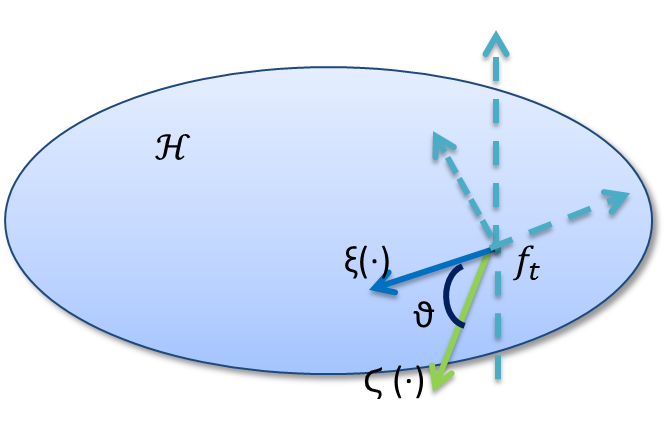
Figure 1: Ο‘italic-Ο‘\vartheta is the angle betwen ξ​(β‹…)πœ‰β‹…\xi(\cdot) and ΢​(β‹…)πœβ‹…\zeta(\cdot), ΢​(β‹…)πœβ‹…\zeta(\cdot) may be outside of β„‹β„‹\mathcal{H}.

Note that the stochastic functional gradient ξ​(β‹…)πœ‰β‹…\xi(\cdot) is in RKHS β„‹β„‹\mathcal{H} but ΢​(β‹…)πœβ‹…\zeta(\cdot) may be outside β„‹β„‹\mathcal{H}, since ϕω​(β‹…)subscriptitalic-Ο•πœ”β‹…\phi_{\omega}(\cdot) may be outside the RKHS. For instance, for the Gaussian RBF kernel, the random feature ϕω​(x)=2​cos⁑(Ο‰βŠ€β€‹x+b)subscriptitalic-Ο•πœ”π‘₯2superscriptπœ”topπ‘₯𝑏\phi_{\omega}(x)=\sqrt{2}\cos(\omega^{\top}x+b) is outside the RKHS associated with the kernel function.

However, these functional gradients are related by ξ​(β‹…)=𝔼ω​[΢​(β‹…)]πœ‰β‹…subscriptπ”Όπœ”delimited-[]πœβ‹…\xi(\cdot)=\mathbb{E}_{\omega}\left[\zeta(\cdot)\right], which lead to unbiased estimators of the original functional gradient,Β i.e.,

βˆ‡R​(f)=𝔼(x,y)​[ξ​(β‹…)]+v​f​(β‹…),βˆ‡π‘…π‘“subscript𝔼π‘₯𝑦delimited-[]πœ‰β‹…π‘£π‘“β‹…\displaystyle\nabla R(f)=\mathbb{E}_{(x,y)}\left[\xi(\cdot)\right]+vf(\cdot), (5)
andβˆ‡R​(f)=𝔼(x,y)​𝔼ω​[΢​(β‹…)]+v​f​(β‹…).andβˆ‡π‘…π‘“subscript𝔼π‘₯𝑦subscriptπ”Όπœ”delimited-[]πœβ‹…π‘£π‘“β‹…\displaystyle\text{and}\quad\nabla R(f)=\mathbb{E}_{(x,y)}\mathbb{E}_{\omega}\left[\zeta(\cdot)\right]+vf(\cdot). (6)

We emphasize that the source of randomness associated with the random feature is not present in the data, but artificially introduced by us. This is crucial for the development of our scalable algorithm in the next section. Meanwhile, it also creates additional challenges in the analysis of the algorithm which we will deal with carefully.

4 Doubly Stochastic Kernel Machines

Β  Algorithm 1: {Ξ±i}i=1t=Train​(ℙ​(x,y))superscriptsubscriptsubscript𝛼𝑖𝑖1𝑑Trainβ„™π‘₯𝑦\left\{\alpha_{i}\right\}_{i=1}^{t}=\text{Train}(\mathbb{P}(x,y)) Β  Require: ℙ​(Ο‰),ϕω​(x),l​(f​(x),y),Ξ½.β„™πœ”subscriptitalic-Ο•πœ”π‘₯𝑙𝑓π‘₯π‘¦πœˆ\mathbb{P}(\omega),\,\phi_{\omega}(x),\,l(f(x),y),\,\nu.

1:Β Β forΒ i=1,…,t𝑖1…𝑑i=1,\ldots,tΒ do
2:Β Β Β Β Β Sample (xi,yi)βˆΌβ„™β€‹(x,y)similar-tosubscriptπ‘₯𝑖subscript𝑦𝑖ℙπ‘₯𝑦(x_{i},y_{i})\sim\mathbb{P}(x,y).
3:Β Β Β Β Β Sample Ο‰iβˆΌβ„™β€‹(Ο‰)similar-tosubscriptπœ”π‘–β„™πœ”\omega_{i}\sim\mathbb{P}(\omega) with seed i𝑖i.
4:Β Β Β Β Β f​(xi)=Predict​(xi,{Ξ±j}j=1iβˆ’1)𝑓subscriptπ‘₯𝑖Predictsubscriptπ‘₯𝑖superscriptsubscriptsubscript𝛼𝑗𝑗1𝑖1f(x_{i})=\text{\bf Predict}(x_{i},\left\{\alpha_{j}\right\}_{j=1}^{i-1}).
5:Β Β Β Β Β Ξ±i=βˆ’Ξ³i​l′​(f​(xi),yi)​ϕωi​(xi)subscript𝛼𝑖subscript𝛾𝑖superscript𝑙′𝑓subscriptπ‘₯𝑖subscript𝑦𝑖subscriptitalic-Ο•subscriptπœ”π‘–subscriptπ‘₯𝑖\alpha_{i}=-\gamma_{i}l^{\prime}(f(x_{i}),y_{i})\phi_{\omega_{i}}(x_{i}).
6:Β Β Β Β Β Ξ±j=(1βˆ’Ξ³i​ν)​αjsubscript𝛼𝑗1subscriptπ›Ύπ‘–πœˆsubscript𝛼𝑗\alpha_{j}=(1-\gamma_{i}\nu)\alpha_{j} for j=1,…,iβˆ’1𝑗1…𝑖1j=1,\ldots,i-1.
7:Β Β endΒ for

Β 

Β  Algorithm 2: f​(x)=Predict​(x,{Ξ±i}i=1t)𝑓π‘₯Predictπ‘₯superscriptsubscriptsubscript𝛼𝑖𝑖1𝑑f(x)=\text{Predict}(x,\,\left\{\alpha_{i}\right\}_{i=1}^{t}) Β  Require: ℙ​(Ο‰),ϕω​(x).β„™πœ”subscriptitalic-Ο•πœ”π‘₯\mathbb{P}(\omega),\,\phi_{\omega}(x).

1:Β Β Set f​(x)=0𝑓π‘₯0f(x)=0.
2:Β Β forΒ i=1,…,t𝑖1…𝑑i=1,\ldots,tΒ do
3:Β Β Β Β Β Sample Ο‰iβˆΌβ„™β€‹(Ο‰)similar-tosubscriptπœ”π‘–β„™πœ”\omega_{i}\sim\mathbb{P}(\omega) with seed i𝑖i.
4:Β Β Β Β Β f​(x)=f​(x)+Ξ±i​ϕωi​(x)𝑓π‘₯𝑓π‘₯subscript𝛼𝑖subscriptitalic-Ο•subscriptπœ”π‘–π‘₯f(x)=f(x)+\alpha_{i}\phi_{\omega_{i}}(x).
5:Β Β endΒ for

Β 

The first key intuition behind our algorithm originates from the property of stochastic gradient descent algorithm that as long as the stochastic gradient is unbiased, the convergence of the algorithm is guaranteedΒ [16]. In our algorithm, we will exploit this property and introduce two sources of randomness, one from data and another artificial, to scale up kernel methods.

The second key intuition behind our algorithm is that the random features used in the doubly stochastic functional gradients will be sampled according to pseudo-random number generators, where the sequences of apparently random samples can in fact be completely determined by an initial value (a seed). Although these random samples are not the β€œtrue” random sample in the purest sense of the word, however they suffice for our task in practice.

More specifically, our algorithm proceeds by making two unbiased stochastic approximation to the functional gradient in each iteration, and then descending using this noisy functional gradient. The overall algorithms for training and prediction is summarized in Algorithm 1 and 2. The training algorithm essentially just performs random feature sampling and doubly stochastic gradient evaluation, and maintains a collection of real number {Ξ±i}subscript𝛼𝑖\left\{\alpha_{i}\right\}, which is computationally efficient and memory friendly. A crucial step in the algorithm is to sample the random features with β€œseed i𝑖i”. The seeds have to be aligned between training and prediction, and with the corresponding Ξ±isubscript𝛼𝑖\alpha_{i} obtained from each iteration. The learning rate Ξ³tsubscript𝛾𝑑\gamma_{t} in the algorithm needs to be chosen as O​(1/t)𝑂1𝑑O(1/t), as shown by our later analysis to achieve the best rate of convergence. For now, we assume that we have access to the data generating distribution ℙ​(x,y)β„™π‘₯𝑦\mathbb{P}(x,y). This can be modified to sample uniformly randomly from a fixed dataset, without affecting the algorithm and the later convergence analysis. Let the sampled data and random feature parameters be π’Ÿt:={(xi,yi)}i=1tassignsuperscriptπ’Ÿπ‘‘superscriptsubscriptsubscriptπ‘₯𝑖subscript𝑦𝑖𝑖1𝑑\mathcal{D}^{t}:=\left\{(x_{i},y_{i})\right\}_{i=1}^{t} and 𝝎t:={Ο‰i}i=1tassignsuperscriptπŽπ‘‘superscriptsubscriptsubscriptπœ”π‘–π‘–1𝑑\bm{\omega}^{t}:=\left\{\omega_{i}\right\}_{i=1}^{t} respectively after t𝑑t iteration, the function obtained by Algorithm 1 is a simple additive form of the doubly stochastic functional gradients

ft+1​(β‹…)=ft​(β‹…)βˆ’Ξ³t​(ΞΆt​(β‹…)+ν​ft​(β‹…))=βˆ‘i=1tati​΢i​(β‹…),βˆ€t>1,andf1​(β‹…)=0,formulae-sequencesubscript𝑓𝑑1β‹…subscript𝑓𝑑⋅subscript𝛾𝑑subscriptπœπ‘‘β‹…πœˆsubscript𝑓𝑑⋅superscriptsubscript𝑖1𝑑superscriptsubscriptπ‘Žπ‘‘π‘–subscriptπœπ‘–β‹…formulae-sequencefor-all𝑑1andsubscript𝑓1β‹…0\displaystyle f_{t+1}(\cdot)=f_{t}(\cdot)-\gamma_{t}(\zeta_{t}(\cdot)+\nu f_{t}(\cdot))=\sum\nolimits_{i=1}^{t}a_{t}^{i}\zeta_{i}(\cdot),\quad\forall t>1,\quad\text{and}\quad f_{1}(\cdot)=0, (7)

where ati=βˆ’Ξ³iβ€‹βˆj=i+1t(1βˆ’Ξ³j​ν)superscriptsubscriptπ‘Žπ‘‘π‘–subscript𝛾𝑖superscriptsubscriptproduct𝑗𝑖1𝑑1subscriptπ›Ύπ‘—πœˆa_{t}^{i}=-\gamma_{i}\prod_{j=i+1}^{t}(1-\gamma_{j}\nu) are deterministic values depending on the step sizes Ξ³j​(iβ©½jβ©½t)subscript𝛾𝑗𝑖𝑗𝑑\gamma_{j}(i\leqslant j\leqslant t) and regularization parameter ν𝜈\nu. This simple form makes it easy for us to analyze its convergence.

We note that our algorithm can also take a mini-batch of points and random features at each step, and estimate an empirical covariance for preconditioning to achieve potentially better performance.

Our algorithm is general and can be applied to most of the kernel machines which are formulated in the convex optimizationΒ (1) in a RKHS β„‹β„‹\mathcal{H} associated with given kernel k​(x,xβ€²)π‘˜π‘₯superscriptπ‘₯β€²k(x,x^{\prime}). We will instantiate the doubly stochastic gradients algorithms for a few commonly used kernel machines for different tasks and loss functions, e.g., regression, classification, quantile regression, novelty detection and estimating divergence functionals/likelihood ratio. Interestingly, the Gaussian process regression, which is a Bayesian model, can also be reformulated as the solution to particular convex optimizations in RKHS, and therefore, be approximated by the proposed algorithm.

Kernel Support Vector MachineΒ (SVM). Hinge loss is used in kernel SVM where l​(u,y)=max⁑{0,1βˆ’u​y}𝑙𝑒𝑦01𝑒𝑦l(u,y)=\max\{0,1-uy\} with y∈{βˆ’1,1}𝑦11y\in\{-1,1\}. We have l′​(u,y)={0if ​y​uβ©Ύ1βˆ’yif ​y​u<1superscript𝑙′𝑒𝑦cases0if 𝑦𝑒1𝑦if 𝑦𝑒1l^{\prime}(u,y)=\begin{cases}0&\,\text{if }yu\geqslant 1\\ -y&\,\text{if }yu<1\\ \end{cases} and the step 5 in Algorithm.Β 1. becomes

Ξ±i={0if ​yi​f​(xi)β©Ύ1Ξ³i​yi​ϕωi​(xi)if ​yi​f​(xi)<1.subscript𝛼𝑖cases0ifΒ subscript𝑦𝑖𝑓subscriptπ‘₯𝑖1subscript𝛾𝑖subscript𝑦𝑖subscriptitalic-Ο•subscriptπœ”π‘–subscriptπ‘₯𝑖ifΒ subscript𝑦𝑖𝑓subscriptπ‘₯𝑖1\alpha_{i}=\begin{cases}0&\,\text{if }y_{i}f(x_{i})\geqslant 1\\ \gamma_{i}y_{i}\phi_{\omega_{i}}(x_{i})&\,\text{if }y_{i}f(x_{i})<1\end{cases}.

Remark: [14] used squared hinge loss, l(u,y)=12max{0,1βˆ’uy}2l(u,y)=\frac{1}{2}\max\{0,1-uy\}^{2}, in β„“2subscriptβ„“2\ell_{2}-SVM. With this loss function, we have l′​(u,y)={0if ​y​uβ©Ύ1uβˆ’yif ​y​u<1superscript𝑙′𝑒𝑦cases0if 𝑦𝑒1𝑒𝑦if 𝑦𝑒1l^{\prime}(u,y)=\begin{cases}0&\,\text{if }yu\geqslant 1\\ u-y&\,\text{if }yu<1\\ \end{cases} and the step 5 in Algorithm.Β 1. becomes

Ξ±i={0if ​yi​f​(xi)β©Ύ1Ξ³i​(yiβˆ’f​(xi))​ϕωi​(xi)if ​yi​f​(xi)<1.subscript𝛼𝑖cases0ifΒ subscript𝑦𝑖𝑓subscriptπ‘₯𝑖1subscript𝛾𝑖subscript𝑦𝑖𝑓subscriptπ‘₯𝑖subscriptitalic-Ο•subscriptπœ”π‘–subscriptπ‘₯𝑖ifΒ subscript𝑦𝑖𝑓subscriptπ‘₯𝑖1\alpha_{i}=\begin{cases}0&\,\text{if }y_{i}f(x_{i})\geqslant 1\\ \gamma_{i}(y_{i}-f(x_{i}))\phi_{\omega_{i}}(x_{i})&\,\text{if }y_{i}f(x_{i})<1\end{cases}.

Kernel Logistic Regression. Log loss is used in kernel logistic regression for binary classification where l​(u,y)=log⁑(1+exp⁑(βˆ’y​u))𝑙𝑒𝑦1𝑦𝑒l(u,y)=\log(1+\exp(-yu)) with y∈{βˆ’1,1}𝑦11y\in\{-1,1\}. We have l′​(u,y)=βˆ’y​exp⁑(βˆ’y​u)1+exp⁑(βˆ’y​u)superscript𝑙′𝑒𝑦𝑦𝑦𝑒1𝑦𝑒l^{\prime}(u,y)=-\frac{y\exp(-yu)}{1+\exp(-yu)} and the step 5 in Algorithm.Β 1. becomes

Ξ±i=Ξ³i​yi​exp⁑(βˆ’yi​f​(xi))1+exp⁑(βˆ’yi​f​(xi))​ϕωi​(xi).subscript𝛼𝑖subscript𝛾𝑖subscript𝑦𝑖subscript𝑦𝑖𝑓subscriptπ‘₯𝑖1subscript𝑦𝑖𝑓subscriptπ‘₯𝑖subscriptitalic-Ο•subscriptπœ”π‘–subscriptπ‘₯𝑖\alpha_{i}=\gamma_{i}y_{i}\frac{\exp(-y_{i}f(x_{i}))}{1+\exp(-y_{i}f(x_{i}))}\phi_{\omega_{i}}(x_{i}).

For the multi-class kernel logistic regression, the l​(u,y)=βˆ’βˆ‘c=1CΞ΄c​(y)​uc+log⁑(βˆ‘c=1Cexp⁑(uc))𝑙𝑒𝑦superscriptsubscript𝑐1𝐢subscript𝛿𝑐𝑦subscript𝑒𝑐superscriptsubscript𝑐1𝐢subscript𝑒𝑐l(u,y)=-\sum_{{c}=1}^{C}\delta_{c}(y)u_{c}+\log\bigg{(}\sum_{{c}=1}^{C}\exp(u_{c})\bigg{)} where C𝐢C is the number of categories, uβˆˆβ„CΓ—1𝑒superscriptℝ𝐢1u\in\mathbb{R}^{C\times 1}, y∈{1,…,C}𝑦1…𝐢y\in\{1,\ldots,C\} and Ξ΄c​(y)=1subscript𝛿𝑐𝑦1\delta_{c}(y)=1 only if y=c𝑦𝑐y=c, otherwise Ξ΄c​(y)=0subscript𝛿𝑐𝑦0\delta_{c}(y)=0. In such scenario, we denote πŸβ€‹(xi)=[f1​(xi),…,fC​(xi)]𝐟subscriptπ‘₯𝑖superscript𝑓1subscriptπ‘₯𝑖…superscript𝑓𝐢subscriptπ‘₯𝑖\mathbf{f}(x_{i})=[f^{1}(x_{i}),\ldots,f^{C}(x_{i})], and therefore, the corresponding 𝜢=[Ξ±1,…,Ξ±C]𝜢superscript𝛼1…superscript𝛼𝐢\bm{\alpha}=[\alpha^{1},\ldots,\alpha^{C}]. The update rule for 𝜢𝜢\bm{\alpha} in Algorithm.Β 1. is

Ξ±icsuperscriptsubscript𝛼𝑖𝑐\displaystyle\alpha_{i}^{c} =\displaystyle= Ξ³i​(Ξ΄c​(yi)βˆ’exp⁑(fc​(xi))βˆ‘c=1Cexp⁑(fc​(xi)))​ϕωi​(xi)βˆ€c=1,…,C,formulae-sequencesubscript𝛾𝑖subscript𝛿𝑐subscript𝑦𝑖superscript𝑓𝑐subscriptπ‘₯𝑖superscriptsubscript𝑐1𝐢superscript𝑓𝑐subscriptπ‘₯𝑖subscriptitalic-Ο•subscriptπœ”π‘–subscriptπ‘₯𝑖for-all𝑐1…𝐢\displaystyle\gamma_{i}\bigg{(}\delta_{c}(y_{i})-\frac{\exp(f^{c}(x_{i}))}{\sum_{c=1}^{C}\exp(f^{c}(x_{i}))}\bigg{)}\phi_{\omega_{i}}(x_{i})\quad\forall c=1,\ldots,C,
Ξ±jcsuperscriptsubscript𝛼𝑗𝑐\displaystyle\alpha_{j}^{c} =\displaystyle= (1βˆ’Ξ³iΞ½)Ξ±jc,βˆ€j<i,βˆ€c=1,…,C.\displaystyle(1-\gamma_{i}\nu)\alpha_{j}^{c}\quad,\forall j<i,\forall c=1,\ldots,C.

Kernel Ridge Regression. Square loss is used in kernel ridge regression where l​(u,y)=12​(uβˆ’y)2𝑙𝑒𝑦12superscript𝑒𝑦2l(u,y)=\frac{1}{2}(u-y)^{2}. We have l′​(u,y)=(uβˆ’y)superscript𝑙′𝑒𝑦𝑒𝑦l^{\prime}(u,y)=(u-y) and the step 5 in Algorithm.Β 1. becomes

Ξ±i=βˆ’Ξ³i​(f​(xi)βˆ’yi)​ϕωi​(xi).subscript𝛼𝑖subscript𝛾𝑖𝑓subscriptπ‘₯𝑖subscript𝑦𝑖subscriptitalic-Ο•subscriptπœ”π‘–subscriptπ‘₯𝑖\alpha_{i}=-\gamma_{i}(f(x_{i})-y_{i})\phi_{\omega_{i}}(x_{i}).

Kernel Robust Regression. Huber’s loss is used for robust regressionΒ [22] where

l​(u,y)={12​(uβˆ’y)2if ​|uβˆ’y|β©½1|uβˆ’y|βˆ’12if ​|uβˆ’y|>1.𝑙𝑒𝑦cases12superscript𝑒𝑦2if 𝑒𝑦1𝑒𝑦12if 𝑒𝑦1l(u,y)=\begin{cases}\frac{1}{2}(u-y)^{2}&\text{if }|u-y|\leqslant 1\\ |u-y|-\frac{1}{2}&\text{if }|u-y|>1\end{cases}.

We have l′​(u,y)={(uβˆ’y)if ​|uβˆ’y|β©½1sign(uβˆ’y)if ​|uβˆ’y|>1superscript𝑙′𝑒𝑦cases𝑒𝑦if 𝑒𝑦1sign𝑒𝑦if 𝑒𝑦1l^{\prime}(u,y)=\begin{cases}(u-y)&\text{if }|u-y|\leqslant 1\\ \mathop{\mathrm{sign}}(u-y)&\text{if }|u-y|>1\end{cases} and the step 5 in Algorithm.Β 1. becomes

Ξ±i={βˆ’Ξ³i​(f​(xi)βˆ’yi)​ϕωi​(xi)if ​|f​(xi)βˆ’yi|β©½1βˆ’Ξ³i​sign(f​(xi)βˆ’yi)​ϕωi​(xi)if ​|f​(xi)βˆ’yi|>1subscript𝛼𝑖casessubscript𝛾𝑖𝑓subscriptπ‘₯𝑖subscript𝑦𝑖subscriptitalic-Ο•subscriptπœ”π‘–subscriptπ‘₯𝑖if 𝑓subscriptπ‘₯𝑖subscript𝑦𝑖1subscript𝛾𝑖sign𝑓subscriptπ‘₯𝑖subscript𝑦𝑖subscriptitalic-Ο•subscriptπœ”π‘–subscriptπ‘₯𝑖if 𝑓subscriptπ‘₯𝑖subscript𝑦𝑖1\alpha_{i}=\begin{cases}-\gamma_{i}(f(x_{i})-y_{i})\phi_{\omega_{i}}(x_{i})&\text{if }|f(x_{i})-y_{i}|\leqslant 1\\ -\gamma_{i}\mathop{\mathrm{sign}}(f(x_{i})-y_{i})\phi_{\omega_{i}}(x_{i})&\text{if }|f(x_{i})-y_{i}|>1\end{cases}

Kernel Support Vector RegressionΒ (SVR). Ο΅italic-Ο΅\epsilon-insensitive loss function is used in kernel SVR where l​(u,y)=max⁑{0,|uβˆ’y|βˆ’Ο΅}𝑙𝑒𝑦0𝑒𝑦italic-Ο΅l(u,y)=\max\{0,|u-y|-\epsilon\}. We have l′​(u,y)={0if ​|uβˆ’y|β©½Ο΅sign(uβˆ’y)if ​|uβˆ’y|>Ο΅superscript𝑙′𝑒𝑦cases0if 𝑒𝑦italic-Ο΅sign𝑒𝑦if 𝑒𝑦italic-Ο΅l^{\prime}(u,y)=\begin{cases}0&\text{if }|u-y|\leqslant\epsilon\\ \mathop{\mathrm{sign}}(u-y)&\text{if }|u-y|>\epsilon\end{cases} and the step 5 in Algorithm.Β 1. becomes

Ξ±i={0if ​|f​(xi)βˆ’yi|β©½Ο΅βˆ’Ξ³i​sign(f​(xi)βˆ’yi)​ϕωi​(xi)if ​|f​(xi)βˆ’yi|>Ο΅subscript𝛼𝑖cases0if 𝑓subscriptπ‘₯𝑖subscript𝑦𝑖italic-Ο΅subscript𝛾𝑖sign𝑓subscriptπ‘₯𝑖subscript𝑦𝑖subscriptitalic-Ο•subscriptπœ”π‘–subscriptπ‘₯𝑖if 𝑓subscriptπ‘₯𝑖subscript𝑦𝑖italic-Ο΅\alpha_{i}=\begin{cases}0&\text{if }|f(x_{i})-y_{i}|\leqslant\epsilon\\ -\gamma_{i}\mathop{\mathrm{sign}}(f(x_{i})-y_{i})\phi_{\omega_{i}}(x_{i})&\text{if }|f(x_{i})-y_{i}|>\epsilon\end{cases}

Remark: Note that if we set Ο΅=0italic-Ο΅0\epsilon=0, the Ο΅italic-Ο΅\epsilon-intensitive loss function will become absolute deviatin, i.e., l​(u,y)=|uβˆ’y|𝑙𝑒𝑦𝑒𝑦l(u,y)=|u-y|. Therefore, we have the updates for kernel least absolute deviatin regression.

Kernel Quantile Regression. The loss function for quantile regression is l​(u,y)=max⁑{τ​(yβˆ’u),(1βˆ’Ο„)​(uβˆ’y)}π‘™π‘’π‘¦πœπ‘¦π‘’1πœπ‘’π‘¦l(u,y)=\max\{\tau(y-u),(1-\tau)(u-y)\}. We have l′​(u,y)={1βˆ’Ο„if ​uβ©Ύyβˆ’Ο„if ​u<ysuperscript𝑙′𝑒𝑦cases1𝜏ifΒ π‘’π‘¦πœif 𝑒𝑦l^{\prime}(u,y)=\begin{cases}1-\tau&\,\text{if }u\geqslant y\\ -\tau&\,\text{if }u<y\\ \end{cases} and the step 5 in Algorithm.Β 1. becomes

Ξ±i={Ξ³i​(Ο„βˆ’1)​ϕωi​(xi)if ​f​(xi)β©ΎyiΞ³i​τ​ϕωi​(xi)if ​f​(xi)<yi.subscript𝛼𝑖casessubscriptπ›Ύπ‘–πœ1subscriptitalic-Ο•subscriptπœ”π‘–subscriptπ‘₯𝑖if 𝑓subscriptπ‘₯𝑖subscript𝑦𝑖subscriptπ›Ύπ‘–πœsubscriptitalic-Ο•subscriptπœ”π‘–subscriptπ‘₯𝑖if 𝑓subscriptπ‘₯𝑖subscript𝑦𝑖\alpha_{i}=\begin{cases}\gamma_{i}(\tau-1)\phi_{\omega_{i}}(x_{i})&\,\text{if }f(x_{i})\geqslant y_{i}\\ \gamma_{i}\tau\phi_{\omega_{i}}(x_{i})&\,\text{if }f(x_{i})<y_{i}\end{cases}.

Kernel Novelty Detection. The loss function l​(u,Ο„)=max⁑{0,Ο„βˆ’u}π‘™π‘’πœ0πœπ‘’l(u,\tau)=\max\{0,\tau-u\}Β [23] is proposed for novelty detection. Since Ο„πœ\tau is also a variable which needs to be optimized, the optimization problem is formulated as

minΟ„βˆˆβ„,fβˆˆβ„‹β‘π”Όx​[l​(f​(x),Ο„)]+Ξ½2​‖fβ€–β„‹2βˆ’Ξ½β€‹Ο„,subscriptformulae-sequenceπœβ„π‘“β„‹subscript𝔼π‘₯delimited-[]𝑙𝑓π‘₯𝜏𝜈2superscriptsubscriptnorm𝑓ℋ2𝜈𝜏\displaystyle\min_{\tau\in\mathbb{R},f\in\mathcal{H}}\mathbb{E}_{x}[l(f(x),\tau)]+\frac{\nu}{2}\|f\|_{\mathcal{H}}^{2}-\nu\tau,

and the gradient of l​(u,Ο„)π‘™π‘’πœl(u,\tau) is

βˆ‚l​(u,Ο„)βˆ‚u={0if ​uβ©ΎΟ„βˆ’1if ​u<Ο„,βˆ‚l​(u,Ο„)βˆ‚Ο„={0if ​uβ©ΎΟ„1if ​u<Ο„.formulae-sequenceπ‘™π‘’πœπ‘’cases0ifΒ π‘’πœ1ifΒ π‘’πœπ‘™π‘’πœπœcases0ifΒ π‘’πœ1ifΒ π‘’πœ\displaystyle\frac{\partial l(u,\tau)}{\partial u}=\begin{cases}0&\,\text{if }u\geqslant\tau\\ -1&\,\text{if }u<\tau\end{cases},\quad\frac{\partial l(u,\tau)}{\partial\tau}=\begin{cases}0&\,\text{if }u\geqslant\tau\\ 1&\,\text{if }u<\tau\end{cases}.

The step 5 in Algorithm.Β 1. becomes

Ξ±i={0if ​f​(xi)β©ΎΟ„iβˆ’1Ξ³i​ϕωi​(xi)if ​f​(xi)<Ο„iβˆ’1,Ο„i={Ο„iβˆ’1+Ξ³i​νif ​f​(xi)β©ΎΟ„iβˆ’1Ο„iβˆ’1βˆ’Ξ³i​(1βˆ’Ξ½)if ​f​(xi)<Ο„iβˆ’1.formulae-sequencesubscript𝛼𝑖cases0if 𝑓subscriptπ‘₯𝑖subscriptπœπ‘–1subscript𝛾𝑖subscriptitalic-Ο•subscriptπœ”π‘–subscriptπ‘₯𝑖if 𝑓subscriptπ‘₯𝑖subscriptπœπ‘–1subscriptπœπ‘–casessubscriptπœπ‘–1subscriptπ›Ύπ‘–πœˆif 𝑓subscriptπ‘₯𝑖subscriptπœπ‘–1subscriptπœπ‘–1subscript𝛾𝑖1𝜈if 𝑓subscriptπ‘₯𝑖subscriptπœπ‘–1\displaystyle\alpha_{i}=\begin{cases}0&\,\text{if }f(x_{i})\geqslant\tau_{i-1}\\ \gamma_{i}\phi_{\omega_{i}}(x_{i})&\,\text{if }f(x_{i})<\tau_{i-1}\end{cases},\quad\tau_{i}=\begin{cases}\tau_{i-1}+\gamma_{i}\nu&\,\text{if }f(x_{i})\geqslant\tau_{i-1}\\ \tau_{i-1}-\gamma_{i}(1-\nu)&\,\text{if }f(x_{i})<\tau_{i-1}\end{cases}.

Kernel Density Ratio Estimation. Based on the variational form of Ali-Silvey divergence, i.e., 𝔼p​[r​(qp)]subscript𝔼𝑝delimited-[]π‘Ÿπ‘žπ‘\mathbb{E}_{p}\big{[}r(\frac{q}{p})\big{]}, where r:ℝ+→ℝ:π‘Ÿβ†’superscriptℝℝr:\mathbb{R}^{+}\rightarrow\mathbb{R} is a convex function with r​(1)=0π‘Ÿ10r(1)=0, [24] proposed a nonparametric estimator for the logarithm of the density ratio, log⁑qpπ‘žπ‘\log\frac{q}{p}, which is the solution of following convex optimization,

argminfβˆˆβ„‹π”Όq​[exp⁑(f)]+𝔼p​[rβˆ—β€‹(βˆ’exp⁑(f))]+Ξ½2​‖fβ€–β„‹2subscriptargmin𝑓ℋsubscriptπ”Όπ‘ždelimited-[]𝑓subscript𝔼𝑝delimited-[]superscriptπ‘Ÿπ‘“πœˆ2superscriptsubscriptnorm𝑓ℋ2\displaystyle\mathop{\mathrm{argmin}}_{f\in\mathcal{H}}~{}~{}\mathbb{E}_{q}[\exp(f)]+\mathbb{E}_{p}[r^{*}(-\exp(f))]+\frac{\nu}{2}\|f\|_{\mathcal{H}}^{2} (8)

where rβˆ—superscriptπ‘Ÿr^{*} denotes the Fenchel-Legendre dual of rπ‘Ÿr, r​(Ο„):=supΟ‡Ο‡β€‹Ο„βˆ’rβˆ—β€‹(Ο‡)assignπ‘Ÿπœsubscriptsupremumπœ’πœ’πœsuperscriptπ‘Ÿπœ’r(\tau):=\sup_{\chi}\chi\tau-r^{*}(\chi). In Kullback-LeiblerΒ (KL) divergence, the rK​L​(Ο„)=βˆ’log⁑(Ο„)subscriptπ‘ŸπΎπΏπœπœr_{KL}(\tau)=-\log(\tau). Its Fenchel-Legendre dual is

rK​Lβˆ—β€‹(Ο„)={∞if ​τ⩾0βˆ’1βˆ’log⁑(βˆ’Ο„)if ​τ<0subscriptsuperscriptπ‘ŸπΎπΏπœcasesif 𝜏01𝜏if 𝜏0\displaystyle r^{*}_{KL}(\tau)=\begin{cases}\infty&\text{if }\tau\geqslant 0\\ -1-\log(-\tau)&\text{if }\tau<0\end{cases}

Specifically, the optimization becomes

minfβˆˆβ„‹β‘R​(f)subscript𝑓ℋ𝑅𝑓\displaystyle\min_{f\in\mathcal{H}}~{}~{}R(f) =\displaystyle= 𝔼y∼q​[exp⁑(f​(y))]βˆ’π”Όx∼p​[f​(x)]+Ξ½2​‖fβ€–β„‹2subscript𝔼similar-toπ‘¦π‘ždelimited-[]𝑓𝑦subscript𝔼similar-toπ‘₯𝑝delimited-[]𝑓π‘₯𝜈2superscriptsubscriptnorm𝑓ℋ2\displaystyle\mathbb{E}_{y\sim q}[\exp(f(y))]-\mathbb{E}_{x\sim p}[f(x)]+\frac{\nu}{2}\|f\|_{\mathcal{H}}^{2}
=\displaystyle= 2​𝔼z,x,y​[Ξ΄1​(z)​exp⁑(f​(y))βˆ’Ξ΄0​(z)​f​(x)]+Ξ½2​‖fβ€–β„‹2.2subscript𝔼𝑧π‘₯𝑦delimited-[]subscript𝛿1𝑧𝑓𝑦subscript𝛿0𝑧𝑓π‘₯𝜈2superscriptsubscriptnorm𝑓ℋ2\displaystyle 2\mathbb{E}_{z,x,y}\bigg{[}\delta_{1}(z)\exp(f(y))-\delta_{0}(z)f(x)\bigg{]}+\frac{\nu}{2}\|f\|_{\mathcal{H}}^{2}.

where z∼Bernoulli​(0.5)similar-to𝑧Bernoulli0.5z\sim\text{Bernoulli}(0.5). Denote l​(ux,uy,z)=Ξ΄1​(z)​exp⁑(uy)βˆ’Ξ΄0​(z)​ux𝑙subscript𝑒π‘₯subscript𝑒𝑦𝑧subscript𝛿1𝑧subscript𝑒𝑦subscript𝛿0𝑧subscript𝑒π‘₯l(u_{x},u_{y},z)=\delta_{1}(z)\exp(u_{y})-\delta_{0}(z)u_{x}, we have

l′​(ux,uy,z)=Ξ΄1​(z)​exp⁑(uy)βˆ’Ξ΄0​(z)superscript𝑙′subscript𝑒π‘₯subscript𝑒𝑦𝑧subscript𝛿1𝑧subscript𝑒𝑦subscript𝛿0𝑧\displaystyle l^{\prime}(u_{x},u_{y},z)=\delta_{1}(z)\exp(u_{y})-\delta_{0}(z)

and the the step 5 in Algorithm.Β 1. becomes

Ξ±i=βˆ’2​γi​(Ξ΄1​(zi)​exp⁑(f​(yi))​ϕωi​(yi)βˆ’Ξ΄0​(zi)​ϕωi​(xi)),zi∼Bernoulli​(0.5).formulae-sequencesubscript𝛼𝑖2subscript𝛾𝑖subscript𝛿1subscript𝑧𝑖𝑓subscript𝑦𝑖subscriptitalic-Ο•subscriptπœ”π‘–subscript𝑦𝑖subscript𝛿0subscript𝑧𝑖subscriptitalic-Ο•subscriptπœ”π‘–subscriptπ‘₯𝑖similar-tosubscript𝑧𝑖Bernoulli0.5\alpha_{i}=-2\gamma_{i}(\delta_{1}(z_{i})\exp(f(y_{i}))\phi_{\omega_{i}}(y_{i})-\delta_{0}(z_{i})\phi_{\omega_{i}}(x_{i})),\quad z_{i}\sim\text{Bernoulli}(0.5).

In particular, the xisubscriptπ‘₯𝑖x_{i} and yisubscript𝑦𝑖y_{i} are not sampled in pair, they are sampled independently from ℙ​(x)β„™π‘₯\mathbb{P}(x) and β„šβ€‹(x)β„šπ‘₯\mathbb{Q}(x) respectively.

[24] proposed another convex optimization based on rK​L​(Ο„)subscriptπ‘ŸπΎπΏπœr_{KL}(\tau) whose solution is a nonparametric estimator for the density ratio. [25] designed rn​v​(Ο„)=max⁑(0,Οβˆ’log⁑τ)subscriptπ‘Ÿπ‘›π‘£πœ0𝜌𝜏r_{nv}(\tau)=\max(0,\rho-\log\tau) for novelty detection. Similarly, the doubly stochastic gradients algorithm is also applicable to these loss functions.

Gaussian Process Regression. The doubly stochastic gradients can be used for approximating the posterior of Gaussian process regression by reformulating the mean and variance of the predictive distribution as the solutions to the convex optimizations with particular loss functions. Let y=f​(x)+ϡ𝑦𝑓π‘₯italic-Ο΅y=f(x)+\epsilon where Ο΅βˆΌπ’©β€‹(0,Οƒ2)similar-toitalic-ϡ𝒩0superscript𝜎2\epsilon\sim\mathcal{N}(0,\sigma^{2}) and f​(x)βˆΌπ’’β€‹π’«β€‹(0,k​(x,xβ€²))similar-to𝑓π‘₯𝒒𝒫0π‘˜π‘₯superscriptπ‘₯β€²f(x)\sim\mathcal{G}\mathcal{P}(0,k(x,x^{\prime})), given the dataset {xi,yi}i=1nsuperscriptsubscriptsubscriptπ‘₯𝑖subscript𝑦𝑖𝑖1𝑛\{x_{i},y_{i}\}_{i=1}^{n}, the posterior distribution of the function at the test point xβˆ—subscriptπ‘₯x_{*} can be derived as

fβˆ—|X,𝐲,xβˆ—βˆΌπ’©β€‹(kβˆ—βŠ€β€‹(K+Οƒ2​I)βˆ’1​𝐲,k​(xβˆ—,xβˆ—)βˆ’kβˆ—βŠ€β€‹(K+Οƒ2​I)βˆ’1​kβˆ—)similar-toconditionalsuperscript𝑓𝑋𝐲superscriptπ‘₯𝒩superscriptsuperscriptπ‘˜topsuperscript𝐾superscript𝜎2𝐼1π²π‘˜superscriptπ‘₯superscriptπ‘₯superscriptsuperscriptπ‘˜topsuperscript𝐾superscript𝜎2𝐼1superscriptπ‘˜\displaystyle f^{*}|X,\mathbf{y},x^{*}\sim\mathcal{N}\left({k^{*}}^{\top}\left(K+\sigma^{2}I\right)^{-1}\mathbf{y},\;k(x^{*},x^{*})-{k^{*}}^{\top}\left(K+\sigma^{2}I\right)^{-1}k^{*}\right) (9)

where Kβˆˆβ„nΓ—n𝐾superscriptℝ𝑛𝑛K\in\mathbb{R}^{n\times n}, Ki​j=K​(xi,xj)subscript𝐾𝑖𝑗𝐾subscriptπ‘₯𝑖subscriptπ‘₯𝑗K_{ij}=K(x_{i},x_{j}), kβˆ—=[k​(xβˆ—,x1),…,k​(xβˆ—,xn)]⊀superscriptπ‘˜superscriptπ‘˜superscriptπ‘₯subscriptπ‘₯1β€¦π‘˜superscriptπ‘₯subscriptπ‘₯𝑛topk^{*}=[k(x^{*},x_{1}),\ldots,k(x^{*},x_{n})]^{\top} and Iβˆˆβ„nΓ—n𝐼superscriptℝ𝑛𝑛I\in\mathbb{R}^{n\times n} is the identity matrix.

Obviously, the posterior mean of the Gaussian process for regression can be thought as the solution to optimization problemΒ (1) with square loss and setting Ξ½=2​σ2𝜈2superscript𝜎2\nu=2\sigma^{2}. Therefore, the update rule for approximating the posterior mean will be the same as kernel ridge regression.

To compute the predictive variance, we need to evaluate the kβˆ—βŠ€β€‹(K+Οƒ2​I)βˆ’1​kβˆ—superscriptsuperscriptπ‘˜topsuperscript𝐾superscript𝜎2𝐼1superscriptπ‘˜{k^{*}}^{\top}\left(K+\sigma^{2}I\right)^{-1}k^{*}. Following, we will introduce two different optimizations whose solutions can be used for evaluating the quantity.

  1. 1.

    Denote Ο•=[k​(x1,β‹…),…,k​(xn,β‹…)]italic-Ο•π‘˜subscriptπ‘₯1β‹…β€¦π‘˜subscriptπ‘₯𝑛⋅\phi=[k(x_{1},\cdot),\ldots,k(x_{n},\cdot)], then

    kβˆ—βŠ€β€‹(K+Οƒ2​I)βˆ’1​kβˆ—superscriptsuperscriptπ‘˜topsuperscript𝐾superscript𝜎2𝐼1superscriptπ‘˜\displaystyle{k^{*}}^{\top}\left(K+\sigma^{2}I\right)^{-1}k^{*} =\displaystyle= k​(xβˆ—,β‹…)βŠ€β€‹Ο•β€‹(Ο•βŠ€β€‹Ο•+Οƒ2​I)βˆ’1β€‹Ο•βŠ€β€‹k​(xβˆ—,β‹…)π‘˜superscriptsuperscriptπ‘₯β‹…topitalic-Ο•superscriptsuperscriptitalic-Ο•topitalic-Ο•superscript𝜎2𝐼1superscriptitalic-Ο•topπ‘˜superscriptπ‘₯β‹…\displaystyle k(x^{*},\cdot)^{\top}\phi\left(\phi^{\top}\phi+\sigma^{2}I\right)^{-1}\phi^{\top}k(x^{*},\cdot)
    =\displaystyle= k​(xβˆ—,β‹…)βŠ€β€‹Ο•β€‹Ο•βŠ€β€‹(Ο•β€‹Ο•βŠ€+Οƒ2​I)βˆ’1​k​(xβˆ—,β‹…)π‘˜superscriptsuperscriptπ‘₯β‹…topitalic-Ο•superscriptitalic-Ο•topsuperscriptitalic-Ο•superscriptitalic-Ο•topsuperscript𝜎2𝐼1π‘˜superscriptπ‘₯β‹…\displaystyle k(x^{*},\cdot)^{\top}\phi\phi^{\top}\left(\phi\phi^{\top}+\sigma^{2}I\right)^{-1}k(x^{*},\cdot)

    where the second equation based on identity (Ο•β€‹Ο•βŠ€+Οƒ2​I)​ϕ=ϕ​(Ο•βŠ€β€‹Ο•+Οƒ2​I)italic-Ο•superscriptitalic-Ο•topsuperscript𝜎2𝐼italic-Ο•italic-Ο•superscriptitalic-Ο•topitalic-Ο•superscript𝜎2𝐼\left(\phi\phi^{\top}+\sigma^{2}I\right)\phi=\phi\left(\phi^{\top}\phi+\sigma^{2}I\right). Therefore, we just need to estimate the operator:

    π’œ=π’žβ€‹(π’ž+Οƒ2n​I)βˆ’1whereπ’ž=1nβ€‹Ο•β€‹Ο•βŠ€=1nβ€‹βˆ‘i=1nk​(xi,β‹…)βŠ—k​(xi,β‹…).formulae-sequenceπ’œπ’žsuperscriptπ’žsuperscript𝜎2𝑛𝐼1whereπ’ž1𝑛italic-Ο•superscriptitalic-Ο•top1𝑛superscriptsubscript𝑖1𝑛tensor-productπ‘˜subscriptπ‘₯π‘–β‹…π‘˜subscriptπ‘₯𝑖⋅\displaystyle\mathcal{A}=\mathcal{C}\left(\mathcal{C}+\frac{\sigma^{2}}{n}I\right)^{-1}\quad\text{where}\quad\mathcal{C}=\frac{1}{n}\phi\phi^{\top}=\frac{1}{n}\sum_{i=1}^{n}k(x_{i},\cdot)\otimes k(x_{i},\cdot). (10)

    We can express π’œπ’œ\mathcal{A} as the solution to the following convex optimization problem

    minπ’œβ‘R​(π’œ)=12​nβ€‹βˆ‘i=1nβ€–k​(xi,β‹…)βˆ’π’œβ€‹k​(xi,β‹…)β€–β„‹2+Οƒ22​nβ€‹β€–π’œβ€–H​S2subscriptπ’œπ‘…π’œ12𝑛superscriptsubscript𝑖1𝑛superscriptsubscriptnormπ‘˜subscriptπ‘₯π‘–β‹…π’œπ‘˜subscriptπ‘₯𝑖⋅ℋ2superscript𝜎22𝑛superscriptsubscriptnormπ’œπ»π‘†2\displaystyle\min_{\mathcal{A}}R(\mathcal{A})=\frac{1}{2n}\sum_{i=1}^{n}\left\|k(x_{i},\cdot)-\mathcal{A}k(x_{i},\cdot)\right\|_{\mathcal{H}}^{2}+\frac{\sigma^{2}}{2n}\left\|\mathcal{A}\right\|_{HS}^{2}

    where βˆ₯β‹…βˆ₯H​S\|\cdot\|_{HS} is the Hilbert-Schmidt norm of the operator. We can achieve the optimum by βˆ‡R=0βˆ‡π‘…0\nabla R=0, which is equivalent to Eq.Β 10.

    Based on this optimization, we approximate the π’œtsubscriptπ’œπ‘‘\mathcal{A}_{t} using βˆ‘iβ©½j,i=1tΞΈi​j​ϕωi​(β‹…)βŠ—Ο•Ο‰j​(β‹…)superscriptsubscriptformulae-sequence𝑖𝑗𝑖1𝑑tensor-productsubscriptπœƒπ‘–π‘—subscriptitalic-Ο•subscriptπœ”π‘–β‹…subscriptitalic-Ο•subscriptπœ”π‘—β‹…\sum_{i\leqslant j,i=1}^{t}\theta_{ij}\phi_{\omega_{i}}(\cdot)\otimes\phi_{\omega_{j}}(\cdot) by doubly stochastic functional gradients. The update rule for ΞΈπœƒ\theta is

    ΞΈi​jsubscriptπœƒπ‘–π‘—\displaystyle\theta_{ij} =\displaystyle= (1βˆ’Οƒ2n​γt)​θi​j,βˆ€iβ©½j<t1superscript𝜎2𝑛subscript𝛾𝑑subscriptπœƒπ‘–π‘—for-all𝑖𝑗𝑑\displaystyle\bigg{(}1-\frac{\sigma^{2}}{n}\gamma_{t}\bigg{)}\theta_{ij},\,\forall i\leqslant j<t
    ΞΈi​tsubscriptπœƒπ‘–π‘‘\displaystyle\theta_{it} =\displaystyle= βˆ’Ξ³tβ€‹βˆ‘jβ©Ύitβˆ’1ΞΈi​j​ϕωj′​(xt)​ϕωt′​(xt),βˆ€i<tsubscript𝛾𝑑superscriptsubscript𝑗𝑖𝑑1subscriptπœƒπ‘–π‘—subscriptitalic-Ο•superscriptsubscriptπœ”π‘—β€²subscriptπ‘₯𝑑subscriptitalic-Ο•superscriptsubscriptπœ”π‘‘β€²subscriptπ‘₯𝑑for-all𝑖𝑑\displaystyle-\gamma_{t}\sum_{j\geqslant i}^{t-1}\theta_{ij}\phi_{\omega_{j}^{\prime}}(x_{t})\phi_{\omega_{t}^{\prime}}(x_{t}),\,\forall i<t
    ΞΈt​tsubscriptπœƒπ‘‘π‘‘\displaystyle\theta_{tt} =\displaystyle= Ξ³t​ϕωt​(xt)​ϕωt′​(xt).subscript𝛾𝑑subscriptitalic-Ο•subscriptπœ”π‘‘subscriptπ‘₯𝑑subscriptitalic-Ο•subscriptsuperscriptπœ”β€²π‘‘subscriptπ‘₯𝑑\displaystyle\gamma_{t}\phi_{\omega_{t}}(x_{t})\phi_{\omega^{\prime}_{t}}(x_{t}).

    Please refer to AppendixΒ D for the details of the derivation.

  2. 2.

    Assume that the testing points, {xiβˆ—}i=1msuperscriptsubscriptsuperscriptsubscriptπ‘₯𝑖𝑖1π‘š\{x_{i}^{*}\}_{i=1}^{m}, are given beforehand, instead of approximating the operator π’œπ’œ\mathcal{A}, we target on functions Fβˆ—=[f1βˆ—,…,fmβˆ—]⊀superscript𝐹superscriptsubscriptsuperscript𝑓1…subscriptsuperscriptπ‘“π‘štopF^{*}=[f^{*}_{1},\ldots,f^{*}_{m}]^{\top} where fiβˆ—β€‹(β‹…)=k​(β‹…)βŠ€β€‹(K+Οƒ2​I)βˆ’1​kiβˆ—subscriptsuperscriptπ‘“π‘–β‹…π‘˜superscriptβ‹…topsuperscript𝐾superscript𝜎2𝐼1superscriptsubscriptπ‘˜π‘–f^{*}_{i}(\cdot)=k(\cdot)^{\top}\left(K+\sigma^{2}I\right)^{-1}k_{i}^{*}, k​(β‹…)=[k​(x1,β‹…),…,k​(x2,β‹…)]π‘˜β‹…π‘˜subscriptπ‘₯1β‹…β€¦π‘˜subscriptπ‘₯2β‹…k(\cdot)=[k(x_{1},\cdot),\ldots,k(x_{2},\cdot)] and kiβˆ—=[k​(xiβˆ—,x1),…,k​(xiβˆ—,xn)]⊀superscriptsubscriptπ‘˜π‘–superscriptπ‘˜superscriptsubscriptπ‘₯𝑖subscriptπ‘₯1β€¦π‘˜superscriptsubscriptπ‘₯𝑖subscriptπ‘₯𝑛topk_{i}^{*}=[k(x_{i}^{*},x_{1}),\ldots,k(x_{i}^{*},x_{n})]^{\top}. Estimating fiβˆ—β€‹(β‹…)subscriptsuperscript𝑓𝑖⋅f^{*}_{i}(\cdot) can be accomplished by solving the optimization problemΒ (1) with square loss and setting yj=k​(xiβˆ—,xj),βˆ€j=1,…,nformulae-sequencesubscriptπ‘¦π‘—π‘˜superscriptsubscriptπ‘₯𝑖subscriptπ‘₯𝑗for-all𝑗1…𝑛y_{j}=k(x_{i}^{*},x_{j}),\forall j=1,\ldots,n, Ξ½=2​σ2𝜈2superscript𝜎2\nu=2\sigma^{2}, leading to the same update rule as kernel ridge regression.

After we obtain these estimators, we can calculate the predictive variance on xiβˆ—superscriptsubscriptπ‘₯𝑖x_{i}^{*} by either k​(xiβˆ—,xiβˆ—)βˆ’π’œβ€‹(xiβˆ—,xiβˆ—)π‘˜superscriptsubscriptπ‘₯𝑖superscriptsubscriptπ‘₯π‘–π’œsuperscriptsubscriptπ‘₯𝑖superscriptsubscriptπ‘₯𝑖k(x_{i}^{*},x_{i}^{*})-\mathcal{A}(x_{i}^{*},x_{i}^{*}) or k​(xiβˆ—,xiβˆ—)βˆ’fiβˆ—β€‹(xiβˆ—)π‘˜superscriptsubscriptπ‘₯𝑖superscriptsubscriptπ‘₯𝑖superscriptsubscript𝑓𝑖superscriptsubscriptπ‘₯𝑖k(x_{i}^{*},x_{i}^{*})-f_{i}^{*}(x_{i}^{*}). We conduct experiments to justify the novel formulations for approximating both the mean and variance of posterior of Gaussian processes for regression, and the doubly stochastic update rule in Section.(7).

Note that, to approximate the operator π’œπ’œ\mathcal{A}, doubly stochastic gradient requires O​(t2)𝑂superscript𝑑2O(t^{2}) memory. Although we do not need to save the whole training dataset, which saves O​(d​t)𝑂𝑑𝑑O(dt) memory cost, this is still computationally expensive. When the mπ‘šm testing data are given, we estimate mπ‘šm functions and each of them requires O​(t)𝑂𝑑O(t) memory cost, the total cost will be O​(t​m)π‘‚π‘‘π‘šO(tm) by the second algorithm.

5 Theoretical Guarantees

In this section, we will show that, both in expectation and with high probability, our algorithm can estimate the optimal function in the RKHS with rate O​(1/t)𝑂1𝑑O(1/t), and achieve a generalization bound of O​(1/t)𝑂1𝑑O(1/\sqrt{t}). The analysis for our algorithm has a new twist compared to previous analysis of stochastic gradient descent algorithms, since the random feature approximation results in an estimator which is outside the RKHS. Besides the analysis for stochastic functional gradient descent, we need to use martingales and the corresponding concentration inequalities to prove that the sequence of estimators, ft+1subscript𝑓𝑑1f_{t+1}, outside the RKHS converge to the optimal function, fβˆ—subscriptπ‘“βˆ—f_{\ast}, in the RKHS. We make the following standard assumptions ahead for later references:

  1. A.

    There exists an optimal solution, denoted as fβˆ—subscript𝑓f_{*}, to the problem of our interest (1).

  2. B.

    Loss function ℓ​(u,y):ℝ×ℝ→ℝ:ℓ𝑒𝑦→ℝℝℝ\ell(u,y):\mathbb{R}\times\mathbb{R}\to\mathbb{R} and its first-order derivative is L𝐿L-Lipschitz continous in terms of the first argument.

  3. C.

    For any data {(xi,yi)}i=1tsuperscriptsubscriptsubscriptπ‘₯𝑖subscript𝑦𝑖𝑖1𝑑\{(x_{i},y_{i})\}_{i=1}^{t} and any trajectory {fi​(β‹…)}i=1tsuperscriptsubscriptsubscript𝑓𝑖⋅𝑖1𝑑\{f_{i}(\cdot)\}_{i=1}^{t}, there exists M>0𝑀0M>0, such that |ℓ′​(fi​(xi),yi)|β©½Msuperscriptβ„“β€²subscript𝑓𝑖subscriptπ‘₯𝑖subscript𝑦𝑖𝑀|\ell^{\prime}(f_{i}(x_{i}),y_{i})|\leqslant M. Note in our situation M𝑀M exists and M<βˆžπ‘€M<\infty since we assume bounded domain and the functions ftsubscript𝑓𝑑f_{t} we generate are always bounded as well.

  4. D.

    There exists ΞΊ>0πœ…0\kappa>0 and Ο•>0italic-Ο•0\phi>0, such that k​(x,xβ€²)β©½ΞΊ,|ϕω​(x)​ϕω​(xβ€²)|β©½Ο•,βˆ€x,xβ€²βˆˆπ’³,Ο‰βˆˆΞ©.formulae-sequenceπ‘˜π‘₯superscriptπ‘₯β€²πœ…formulae-sequencesubscriptitalic-Ο•πœ”π‘₯subscriptitalic-Ο•πœ”superscriptπ‘₯β€²italic-Ο•for-allπ‘₯formulae-sequencesuperscriptπ‘₯β€²π’³πœ”Ξ©k(x,x^{\prime})\leqslant\kappa,\,|\phi_{\omega}(x)\phi_{\omega}(x^{\prime})|\leqslant\phi,\forall x,x^{\prime}\in\mathcal{X},\omega\in\Omega. For example, when k​(β‹…,β‹…)π‘˜β‹…β‹…k(\cdot,\cdot) is the Gaussian RBF kernel, we have ΞΊ=1πœ…1\kappa=1, Ο•=2italic-Ο•2\phi=2.

We now present our main theorems as below. Due to the space restrictions, we will only provide a short sketch of proofs here. The full proofs for the these theorems are given in the AppendixΒ A-C.

Theorem 4 (Convergence in expectation)

When Ξ³t=ΞΈtsubscriptπ›Ύπ‘‘πœƒπ‘‘\gamma_{t}=\frac{\theta}{t} with ΞΈ>0πœƒ0\theta>0 such that ΞΈβ€‹Ξ½βˆˆ(1,2)βˆͺβ„€+πœƒπœˆ12subscriptβ„€\theta\nu\in(1,2)\cup\mathbb{Z}_{+},

π”Όπ’Ÿt,𝝎t​[|ft+1​(x)βˆ’fβˆ—β€‹(x)|2]β©½2​C2+2​κ​Q12t,for anyΒ xβˆˆπ’³subscript𝔼superscriptπ’Ÿπ‘‘superscriptπŽπ‘‘delimited-[]superscriptsubscript𝑓𝑑1π‘₯subscriptπ‘“βˆ—π‘₯22superscript𝐢22πœ…superscriptsubscript𝑄12𝑑for anyΒ xβˆˆπ’³\mathbb{E}_{\mathcal{D}^{t},\bm{\omega}^{t}}\left[|f_{t+1}(x)-f_{\ast}(x)|^{2}\right]\leqslant\frac{2C^{2}+2\kappa Q_{1}^{2}}{t},\quad\text{for any $x\in\mathcal{X}$}

where Q1=max⁑{β€–fβˆ—β€–β„‹,(Q0+Q02+(2β€‹ΞΈβ€‹Ξ½βˆ’1)​(1+θ​ν)2​θ2​κ​M2)/(2β€‹Ξ½β€‹ΞΈβˆ’1)}subscript𝑄1subscriptnormsubscriptπ‘“βˆ—β„‹subscript𝑄0superscriptsubscript𝑄022πœƒπœˆ1superscript1πœƒπœˆ2superscriptπœƒ2πœ…superscript𝑀22πœˆπœƒ1Q_{1}=\max\left\{\left\|f_{\ast}\right\|_{\mathcal{H}},(Q_{0}+\sqrt{Q_{0}^{2}+(2\theta\nu-1)(1+\theta\nu)^{2}\theta^{2}\kappa M^{2}})/(2\nu\theta-1)\right\}, with Q0=2​2​κ1/2​(ΞΊ+Ο•)​L​M​θ2subscript𝑄022superscriptπœ…12πœ…italic-ϕ𝐿𝑀superscriptπœƒ2Q_{0}=2\sqrt{2}\kappa^{1/2}(\kappa+\phi)LM\theta^{2}, and C2=4​(ΞΊ+Ο•)2​M2​θ2superscript𝐢24superscriptπœ…italic-Ο•2superscript𝑀2superscriptπœƒ2C^{2}=4(\kappa+\phi)^{2}M^{2}\theta^{2}.

Theorem 5 (Convergence with high probability)

When Ξ³t=ΞΈtsubscriptπ›Ύπ‘‘πœƒπ‘‘\gamma_{t}=\frac{\theta}{t} with ΞΈ>0πœƒ0\theta>0 such that ΞΈβ€‹Ξ½βˆˆβ„€+πœƒπœˆsubscriptβ„€\theta\nu\in\mathbb{Z}_{+} and tβ©ΎΞΈβ€‹Ξ½π‘‘πœƒπœˆt\geqslant\theta\nu, for any xβˆˆπ’³π‘₯𝒳x\in\mathcal{X}, we have with probability at least 1βˆ’3​δ13𝛿1-3\delta over (π’Ÿt,π›št)superscriptπ’Ÿπ‘‘superscriptπ›šπ‘‘(\mathcal{D}^{t},\bm{\omega}^{t}),

|ft+1​(x)βˆ’fβˆ—β€‹(x)|2β©½C2​ln⁑(2/Ξ΄)t+2​κ​Q22​ln⁑(2​t/Ξ΄)​ln2⁑(t)t,superscriptsubscript𝑓𝑑1π‘₯subscriptπ‘“βˆ—π‘₯2superscript𝐢22𝛿𝑑2πœ…superscriptsubscript𝑄222𝑑𝛿superscript2𝑑𝑑|f_{t+1}(x)-f_{\ast}(x)|^{2}\leqslant\frac{C^{2}\ln(2/\delta)}{t}+\frac{2\kappa Q_{2}^{2}\ln(2t/\delta)\ln^{2}(t)}{t},

where C𝐢C is as above and Q2=max⁑{β€–fβˆ—β€–β„‹,Q0+Q02+κ​M2​(1+θ​ν)2​(ΞΈ2+16​θ/Ξ½)}subscript𝑄2subscriptnormsubscriptπ‘“βˆ—β„‹subscript𝑄0superscriptsubscript𝑄02πœ…superscript𝑀2superscript1πœƒπœˆ2superscriptπœƒ216πœƒπœˆQ_{2}=\max\left\{\left\|f_{\ast}\right\|_{\mathcal{H}},Q_{0}+\sqrt{Q_{0}^{2}+\kappa M^{2}(1+\theta\nu)^{2}(\theta^{2}+16\theta/\nu)}\right\}, with Q0=4​2​κ1/2​M​θ​(8+(ΞΊ+Ο•)​θ​L)subscript𝑄042superscriptπœ…12π‘€πœƒ8πœ…italic-Ο•πœƒπΏQ_{0}=4\sqrt{2}\kappa^{1/2}M\theta(8+(\kappa+\phi)\theta L).

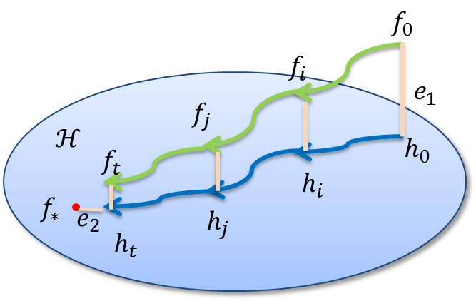
ProofΒ sketch: We focus on the convergence in expectation; the high probability bound can be established in a similar fashion. The main technical difficulty is that ft+1subscript𝑓𝑑1f_{t+1} may not be in the RKHS β„‹β„‹\mathcal{H}. The key of the proof is then to construct an intermediate function ht+1subscriptβ„Žπ‘‘1h_{t+1}, such that the difference between ft+1subscript𝑓𝑑1f_{t+1} and ht+1subscriptβ„Žπ‘‘1h_{t+1} and the difference between ht+1subscriptβ„Žπ‘‘1h_{t+1} and fβˆ—subscript𝑓f_{*} can be bounded. More specifically,

ht+1​(β‹…)=ht​(β‹…)βˆ’Ξ³t​(ΞΎt​(β‹…)+ν​ht​(β‹…))=βˆ‘i=1tati​ξi​(β‹…),βˆ€t>1,andh1​(β‹…)=0,formulae-sequencesubscriptβ„Žπ‘‘1β‹…subscriptβ„Žπ‘‘β‹…subscript𝛾𝑑subscriptπœ‰π‘‘β‹…πœˆsubscriptβ„Žπ‘‘β‹…superscriptsubscript𝑖1𝑑superscriptsubscriptπ‘Žπ‘‘π‘–subscriptπœ‰π‘–β‹…formulae-sequencefor-all𝑑1andsubscriptβ„Ž1β‹…0\displaystyle h_{t+1}(\cdot)=h_{t}(\cdot)-\gamma_{t}(\xi_{t}(\cdot)+\nu h_{t}(\cdot))=\sum\nolimits_{i=1}^{t}a_{t}^{i}\xi_{i}(\cdot),\quad\forall t>1,\quad\text{and}\quad h_{1}(\cdot)=0, (11)

where ΞΎt​(β‹…)=𝔼ωt​[ΞΆt​(β‹…)]subscriptπœ‰π‘‘β‹…subscript𝔼subscriptπœ”π‘‘delimited-[]subscriptπœπ‘‘β‹…\xi_{t}(\cdot)=\mathbb{E}_{\omega_{t}}[\zeta_{t}(\cdot)]. Then for any xπ‘₯x, the error can be decomposed as two terms

|ft+1​(x)βˆ’fβˆ—β€‹(x)|2β©½2​|ft+1​(x)βˆ’ht+1​(x)|2⏟ error due to random features+2​κ​‖ht+1βˆ’fβˆ—β€–β„‹2⏟error due to random datasuperscriptsubscript𝑓𝑑1π‘₯subscriptπ‘“βˆ—π‘₯22subscript⏟superscriptsubscript𝑓𝑑1π‘₯subscriptβ„Žπ‘‘1π‘₯2Β error due to random features2πœ…subscript⏟superscriptsubscriptnormsubscriptβ„Žπ‘‘1subscriptπ‘“βˆ—β„‹2error due to random data\displaystyle|f_{t+1}(x)-f_{\ast}(x)|^{2}\leqslant 2\underbrace{|f_{t+1}(x)-h_{t+1}(x)|^{2}}_{\text{ error due to random features}}~{}~{}~{}~{}+~{}~{}~{}~{}2\kappa\underbrace{\left\|h_{t+1}-f_{\ast}\right\|_{\mathcal{H}}^{2}}_{\text{error due to random data}}

For the error term due to random features, ht+1subscriptβ„Žπ‘‘1h_{t+1} is constructed such that ft+1βˆ’ht+1subscript𝑓𝑑1subscriptβ„Žπ‘‘1f_{t+1}-h_{t+1} is a martingale, and the stepsizes are chosen such that |ati|β©½ΞΈtsuperscriptsubscriptπ‘Žπ‘‘π‘–πœƒπ‘‘|a_{t}^{i}|\leqslant\frac{\theta}{t}, which allows us to bound the martingale. In other words, the choices of the stepsizes keep ft+1subscript𝑓𝑑1f_{t+1} close to the RKHS. For the error term due to random data, since ht+1βˆˆβ„‹subscriptβ„Žπ‘‘1β„‹h_{t+1}\in\mathcal{H}, we can now apply the standard arguments for stochastic approximation in the RKHS. Due to the additional randomness, the recursion is slightly more complicated, et+1β©½(1βˆ’2​ν​θt)​et+Ξ²1t​ett+Ξ²2t2,subscript𝑒𝑑112πœˆπœƒπ‘‘subscript𝑒𝑑subscript𝛽1𝑑subscript𝑒𝑑𝑑subscript𝛽2superscript𝑑2e_{t+1}\leqslant\left(1-\frac{2\nu\theta}{t}\right)e_{t}+\frac{\beta_{1}}{t}\sqrt{\frac{e_{t}}{t}}+\frac{\beta_{2}}{t^{2}}, where et+1=π”Όπ’Ÿt,𝝎t​[β€–ht+1βˆ’fβˆ—β€–β„‹2]subscript𝑒𝑑1subscript𝔼superscriptπ’Ÿπ‘‘superscriptπŽπ‘‘delimited-[]superscriptsubscriptnormsubscriptβ„Žπ‘‘1subscript𝑓ℋ2e_{t+1}=\mathbb{E}_{\mathcal{D}^{t},\bm{\omega}^{t}}[\|h_{t+1}-f_{*}\|_{\mathcal{H}}^{2}], and Ξ²1subscript𝛽1\beta_{1} and Ξ²2subscript𝛽2\beta_{2} depends on the related parameters. Solving this recursion then leads to a bound for the second error term. Β 
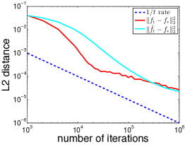
Refer to caption
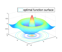
Figure 2: e1subscript𝑒1e_{1} stands the error due to random features, and e2subscript𝑒2e_{2} stands for the error due to random data.
Theorem 6 (Generalization bound)

Let the true risk be Rt​r​u​e​(f)=𝔼(x,y)​[l​(f​(x),y)]subscriptπ‘…π‘‘π‘Ÿπ‘’π‘’π‘“subscript𝔼π‘₯𝑦delimited-[]𝑙𝑓π‘₯𝑦R_{true}(f)=\mathbb{E}_{(x,y)}\left[l(f(x),y)\right]. Then with probability at least 1βˆ’3​δ13𝛿1-3\delta over (π’Ÿt,π›št)superscriptπ’Ÿπ‘‘superscriptπ›šπ‘‘(\mathcal{D}^{t},\bm{\omega}^{t}), and C𝐢C and Q2subscript𝑄2Q_{2} defined as previously

Rt​r​u​e​(ft+1)βˆ’Rt​r​u​e​(fβˆ—)β©½(C​ln⁑(8​e​t/Ξ΄)+2​κ​Q2​ln⁑(2​t/Ξ΄)​ln⁑(t))​Lt.subscriptπ‘…π‘‘π‘Ÿπ‘’π‘’subscript𝑓𝑑1subscriptπ‘…π‘‘π‘Ÿπ‘’π‘’subscript𝑓𝐢8𝑒𝑑𝛿2πœ…subscript𝑄22𝑑𝛿𝑑𝐿𝑑R_{true}(f_{t+1})-R_{true}(f_{*})\leqslant\frac{(C\sqrt{\ln(8\sqrt{e}t/\delta)}+\sqrt{2\kappa}Q_{2}\sqrt{\ln(2t/\delta)}\ln(t))L}{\sqrt{t}}.

ProofΒ  By the Lipschitz continuity of l​(β‹…,y)𝑙⋅𝑦l(\cdot,y) and Jensen’s Inequality, we have

Rt​r​u​e​(ft+1)βˆ’Rt​r​u​e​(fβˆ—)β©½L​𝔼x​|ft+1​(x)βˆ’fβˆ—β€‹(x)|β©½L​𝔼x​|ft+1​(x)βˆ’fβˆ—β€‹(x)|2=L​‖ft+1βˆ’fβˆ—β€–2.subscriptπ‘…π‘‘π‘Ÿπ‘’π‘’subscript𝑓𝑑1subscriptπ‘…π‘‘π‘Ÿπ‘’π‘’subscript𝑓𝐿subscript𝔼π‘₯subscript𝑓𝑑1π‘₯subscript𝑓π‘₯𝐿subscript𝔼π‘₯superscriptsubscript𝑓𝑑1π‘₯subscript𝑓π‘₯2𝐿subscriptnormsubscript𝑓𝑑1subscript𝑓2R_{true}(f_{t+1})-R_{true}(f_{*})\leqslant L\mathbb{E}_{x}|f_{t+1}(x)-f_{*}(x)|\leqslant L\sqrt{\mathbb{E}_{x}|f_{t+1}(x)-f_{*}(x)|^{2}}=L\|f_{t+1}-f_{*}\|_{2}.

Again, β€–ft+1βˆ’fβˆ—β€–2subscriptnormsubscript𝑓𝑑1subscript𝑓2\|f_{t+1}-f_{*}\|_{2} can be decomposed as two terms O​(β€–ft+1βˆ’ht+1β€–22)𝑂superscriptsubscriptnormsubscript𝑓𝑑1subscriptβ„Žπ‘‘122O\left(\|f_{t+1}-h_{t+1}\|_{2}^{2}\right) and O​(β€–ht+1βˆ’fβˆ—β€–β„‹2)𝑂superscriptsubscriptnormsubscriptβ„Žπ‘‘1subscriptπ‘“βˆ—β„‹2O(\left\|h_{t+1}-f_{\ast}\right\|_{\mathcal{H}}^{2}), which can be bounded similarly as in TheoremΒ 5 (see CorollaryΒ 12 in the appendix). Β 
Remarks. The overall rate of convergence in expectation, which is O​(1/t)𝑂1𝑑O(1/t), is indeed optimal. Classical complexity theory (see, e.g. reference inΒ [16]) shows that to obtain Ο΅italic-Ο΅\epsilon-accuracy solution, the number of iterations needed for the stochastic approximation is Ω​(1/Ο΅)Ξ©1italic-Ο΅\Omega(1/\epsilon) for strongly convex case and Ω​(1/Ο΅2)Ξ©1superscriptitalic-Ο΅2\Omega(1/\epsilon^{2}) for general convex case. Different from the classical setting of stochastic approximation, our case imposes not one but two sources of randomness/stochasticity in the gradient, which intuitively speaking, might require higher order number of iterations for general convex case. However, the variance of the random features only contributes additively to the constant in the final convergence rate. Therefore, our method is still able to achieve the same rate as in the classical setting. Notice that these bounds are achieved by adopting the classical stochastic gradient algorithm, and they may be further refined with more sophisticated techniques and analysis. For example, techniques for reducing variance of SGD proposed inΒ [37], mini-batch and preconditioningΒ [41, 42] can be used to reduce the constant factors in the bound significantly. Theorem 4 also reveals bounds in L∞subscript𝐿L_{\infty} and L2subscript𝐿2L_{2} sense as in AppendixΒ B. The choices of stepsizes Ξ³tsubscript𝛾𝑑\gamma_{t} and the tuning parameters given in these bounds are only for sufficient conditions and simple analysis; other choices can also lead to bounds in the same order.

6 Computation, Memory and Statistics Trade-off

To investigate computation, memory and statistics trade-off, we will fix the desired L2subscript𝐿2L_{2} error in the function estimation to Ο΅italic-Ο΅\epsilon,Β i.e., β€–fβˆ’fβˆ—β€–22β©½Ο΅superscriptsubscriptnorm𝑓subscript𝑓22italic-Ο΅\|f-f_{*}\|_{2}^{2}\leqslant\epsilon, and work out the dependency of other quantities on Ο΅italic-Ο΅\epsilon. These other quantities include the preprocessing time, the number of samples and random features (or rank), the number of iterations of each algorithm, and the computational cost and memory requirement for learning and prediction. We assume that the number of samples, n𝑛n, needed to achieve the prescribed error Ο΅italic-Ο΅\epsilon is of the order O​(1/Ο΅)𝑂1italic-Ο΅O(1/\epsilon), the same for all methods. Furthermore, we make no other regularity assumption about margin properties or the kernel matrix such as fast spectrum decay. Thus the required number of random feature (or ranks), rπ‘Ÿr, will be of the order O​(n)=O​(1/Ο΅)𝑂𝑛𝑂1italic-Ο΅O(n)=O(1/\epsilon)Β [4, 5, 8, 9].

We will pick a few representative algorithms for comparison, namely, (i) NORMAΒ [13]: kernel methods trained with stochastic functional gradients; (ii) k-SDCAΒ [12]: kernelized version of stochastic dual coordinate ascend; (iii) r-SDCA: first approximate the kernel function with random features, and then run stochastic dual coordinate ascend; (iv) n-SDCA: first approximate the kernel matrix using NystrΓΆm’s method, and then run stochastic dual coordinate ascend; similarly we will combine Pegasos algorithmΒ [26], stochastic block mirror descent (SBMD)Β [38], and random block coordinate descent (RBCD)Β [39] with random features and NystrΓΆm’s method, and obtain (v) r-Pegasos, (vi) n-Pegasos, (vii) r-SBMD, (viii) n-SBMD, (ix) r-RBCD, and (x) n-RBCD, respectively. The comparisons are summarized below in Table.Β 2111We only considered general kernel algorithms in this section. For some specific loss functions, e.g., hinge-loss, there are algorithms proposed to achieve better memory saving with extra training cost, such as support vector reduction techniqueΒ [40].

Table 2: Comparison of Computation and Memory Requirements
Algorithms Preprocessing Total Computation Cost Total Memory Cost
Computation Training Prediction Training Prediction
Doubly SGD O​(1)𝑂1O(1) O​(d/Ο΅2)𝑂𝑑superscriptitalic-Ο΅2O(d/\epsilon^{2}) O​(d/Ο΅)𝑂𝑑italic-Ο΅O(d/\epsilon) O​(1/Ο΅)𝑂1italic-Ο΅O(1/\epsilon) O​(1/Ο΅)𝑂1italic-Ο΅O(1/\epsilon)
NORMA O​(1)𝑂1O(1) O​(d/Ο΅2)𝑂𝑑superscriptitalic-Ο΅2O(d/\epsilon^{2}) O​(d/Ο΅)𝑂𝑑italic-Ο΅O(d/\epsilon) O​(d/Ο΅)𝑂𝑑italic-Ο΅O(d/\epsilon) O​(d/Ο΅)𝑂𝑑italic-Ο΅O(d/\epsilon)
k-SDCA O​(1)𝑂1O(1) O​(d/Ο΅2​log⁑(1Ο΅))𝑂𝑑superscriptitalic-Ο΅21italic-Ο΅O(d/\epsilon^{2}\log(\frac{1}{\epsilon})) O​(d/Ο΅)𝑂𝑑italic-Ο΅O(d/\epsilon) O​(d/Ο΅)𝑂𝑑italic-Ο΅O(d/\epsilon) O​(d/Ο΅)𝑂𝑑italic-Ο΅O(d/\epsilon)
r-SDCA O​(1)𝑂1O(1) O​(d/Ο΅2​log⁑(1Ο΅))𝑂𝑑superscriptitalic-Ο΅21italic-Ο΅O(d/\epsilon^{2}\log(\frac{1}{\epsilon})) O​(d/Ο΅)𝑂𝑑italic-Ο΅O(d/\epsilon) O​(1/Ο΅)𝑂1italic-Ο΅O(1/\epsilon) O​(1/Ο΅)𝑂1italic-Ο΅O(1/\epsilon)
n-SDCA O​(1/Ο΅3)𝑂1superscriptitalic-Ο΅3O(1/\epsilon^{3}) O​(d/Ο΅2​log⁑(1Ο΅))𝑂𝑑superscriptitalic-Ο΅21italic-Ο΅O(d/\epsilon^{2}\log(\frac{1}{\epsilon})) O​(d/Ο΅)𝑂𝑑italic-Ο΅O(d/\epsilon) O​(1/Ο΅)𝑂1italic-Ο΅O(1/\epsilon) O​(1/Ο΅)𝑂1italic-Ο΅O(1/\epsilon)
r-Pegasos O​(1)𝑂1O(1) O​(d/Ο΅2)𝑂𝑑superscriptitalic-Ο΅2O(d/\epsilon^{2}) O​(d/Ο΅)𝑂𝑑italic-Ο΅O(d/\epsilon) O​(1/Ο΅)𝑂1italic-Ο΅O(1/\epsilon) O​(1/Ο΅)𝑂1italic-Ο΅O(1/\epsilon)
n-Pegasos O​(1/Ο΅3)𝑂1superscriptitalic-Ο΅3O(1/\epsilon^{3}) O​(d/Ο΅2)𝑂𝑑superscriptitalic-Ο΅2O(d/\epsilon^{2}) O​(d/Ο΅)𝑂𝑑italic-Ο΅O(d/\epsilon) O​(1/Ο΅)𝑂1italic-Ο΅O(1/\epsilon) O​(1/Ο΅)𝑂1italic-Ο΅O(1/\epsilon)
r-SBMD O​(1)𝑂1O(1) O​(d/Ο΅2)𝑂𝑑superscriptitalic-Ο΅2O(d/\epsilon^{2}) O​(d/Ο΅)𝑂𝑑italic-Ο΅O(d/\epsilon) O​(1/Ο΅)𝑂1italic-Ο΅O(1/\epsilon) O​(1/Ο΅)𝑂1italic-Ο΅O(1/\epsilon)
n-SBMD O​(1/Ο΅3)𝑂1superscriptitalic-Ο΅3O(1/\epsilon^{3}) O​(d/Ο΅2)𝑂𝑑superscriptitalic-Ο΅2O(d/\epsilon^{2}) O​(d/Ο΅)𝑂𝑑italic-Ο΅O(d/\epsilon) O​(1/Ο΅)𝑂1italic-Ο΅O(1/\epsilon) O​(1/Ο΅)𝑂1italic-Ο΅O(1/\epsilon)
r-RBCD O​(1)𝑂1O(1) O​(d/Ο΅2​log⁑(1Ο΅))𝑂𝑑superscriptitalic-Ο΅21italic-Ο΅O(d/\epsilon^{2}\log(\frac{1}{\epsilon})) O​(d/Ο΅)𝑂𝑑italic-Ο΅O(d/\epsilon) O​(1/Ο΅)𝑂1italic-Ο΅O(1/\epsilon) O​(1/Ο΅)𝑂1italic-Ο΅O(1/\epsilon)
n-RBCD O​(1/Ο΅3)𝑂1superscriptitalic-Ο΅3O(1/\epsilon^{3}) O​(d/Ο΅2​log⁑(1Ο΅))𝑂𝑑superscriptitalic-Ο΅21italic-Ο΅O(d/\epsilon^{2}\log(\frac{1}{\epsilon})) O​(d/Ο΅)𝑂𝑑italic-Ο΅O(d/\epsilon) O​(1/Ο΅)𝑂1italic-Ο΅O(1/\epsilon) O​(1/Ο΅)𝑂1italic-Ο΅O(1/\epsilon)
Table 3: Comparison of Computation and Memory Requirement Per Iteration. b𝑏b denotes the block size in algorithms SBMD and RBCD.
Algorithms Computation per Iteration Memory per Iteration Iteration #
Doubly SGD Ξ˜β€‹(d​t+t+t)Ξ˜π‘‘π‘‘π‘‘π‘‘\Theta(dt+t+t) Ξ˜β€‹(t)Ξ˜π‘‘\Theta(t) O​(1/Ο΅)𝑂1italic-Ο΅O(1/\epsilon)
r-SDCA Ξ˜β€‹(d​n+n+n)Ξ˜π‘‘π‘›π‘›π‘›\Theta(dn+n+n) Ξ˜β€‹(n)Ξ˜π‘›\Theta(n) O​(1/ϡ​log⁑(1Ο΅))𝑂1italic-Ο΅1italic-Ο΅O(1/\epsilon\log(\frac{1}{\epsilon}))
r-Pegasos Ξ˜β€‹(d​n+n+n)Ξ˜π‘‘π‘›π‘›π‘›\Theta(dn+n+n) Ξ˜β€‹(n)Ξ˜π‘›\Theta(n) O​(1/Ο΅)𝑂1italic-Ο΅O(1/\epsilon)
r-SBMD Ξ˜β€‹(d​n+n+n/b)Ξ˜π‘‘π‘›π‘›π‘›π‘\Theta(dn+n+n/b) Ξ˜β€‹(n)Ξ˜π‘›\Theta(n) O​(b/Ο΅)𝑂𝑏italic-Ο΅O(b/\epsilon)
r-RBCD Ξ˜β€‹(d​n2+n2+n/b)Ξ˜π‘‘superscript𝑛2superscript𝑛2𝑛𝑏\Theta(dn^{2}+n^{2}+n/b) Ξ˜β€‹(n)Ξ˜π‘›\Theta(n) O​(log⁑(1/Ο΅))𝑂1italic-Ο΅O(\log(1/\epsilon))

From TableΒ 2, one can see that our method, r-SDCA, r-Pegasos, r-SBMD and r-RBCD achieve the best dependency on the dimension, d𝑑d, of the data up to a log factor. However, often one is interested in increasing the number of random features as more data points are observed to obtain a better generalization ability, e.g., in streaming setting. Then special procedures need to be designed for updating the r-SDCA, r-Pegasos, r-SBMD and r-RBCD solutions, which is not clear how to do easily and efficiently with theoretical guarantees. As a more refined comparison, our algorithm is also the cheapest in terms of per training iteration computation and memory requirement. We list the computational and memory requirements at a particular iteration t<n𝑑𝑛t<n for these five algorithms to achieve Ο΅italic-Ο΅\epsilon error in TableΒ 3.

7 Experiments

We show that our method compares favorably to other scalable kernel methods in medium scale datasets, and neural nets in large scale datasets. Below is a summary of the datasets used. A β€œyes” for the last column means that virtual examples (random cropping and mirror imaging of the original pictures) are generated for training. K-ridge stands for kernel ridge regression; GPR stands for Gaussian processes regression; K-SVM stands for kernel SVM; K-logistic stands for kernel logistic regression.

Table 4: Datasets
Name Model # of samples Input dim Output range Virtual
(1) Synthetic GPR 211superscript2112^{11} 222 [βˆ’1,1.3]11.3[-1,1.3] no
(2) Synthetic K-ridge 220superscript2202^{20} 222 [βˆ’1,1.3]11.3[-1,1.3] no
(3) Adult K-SVM 32K 123 {βˆ’1,1}11\left\{-1,1\right\} no
(4) MNIST 8M 8 vs. 6 K-SVM 1.6M 784 {βˆ’1,1}11\left\{-1,1\right\} yes
(5) Forest K-SVM 0.5M 54 {βˆ’1,1}11\left\{-1,1\right\} no
(6) MNIST 8M K-logistic 8M 1568 {0,…,9}0…9\left\{0,\ldots,9\right\} yes
(7) CIFAR 10 K-logistic 60K 2304 {0,…,9}0…9\left\{0,\ldots,9\right\} yes
(8) ImageNet K-logistic 1.3M 9216 {0,…,999}0…999\left\{0,\ldots,999\right\} yes
(9) QuantumMachine K-ridge 6K 276 [βˆ’800,βˆ’2000]8002000[-800,-2000] yes
(10) MolecularSpace K-ridge 2.3M 2850 [0,13]013[0,13] no

Experiment settings.

We first justify the doubly stochastic algorithm for Gaussian processes regression on dataset (1), comparing with NORMA. The dataset is medium size, so that the closed-form for posterior is tractable. For the large-scale datasets (2) β€” (5), we compare with the first seven algorithms for solving kernel methods discussed in TableΒ 2. For the algorithms based on low rank kernel matrix approximation and random features, i.e., pegasos and SDCA, we set the rank rπ‘Ÿr or number of random features rπ‘Ÿr to be 28superscript282^{8}. We use the same batch size for both our algorithms and the competitors. We adopted two stopping criteria for different purposes. We first stopped the algorithms when they pass through the entire dataset once (SC1). This stopping criterion is designed for justifying our motivation. By investigating the performances of these algorithms with different levels of random feature approximations but the same number of training samples, we could identify that the bottleneck of the performances of the vanilla methods with explicit feature will be their approximation ability. To further demonstrate the advantages of the proposed algorithm in computational cost, we also conduct experiments on datasets (3) – (5) running the competitors within the same time budget as the proposed algorithm (SC2). We do not count the preprocessing time of NystrΓΆm’s method for n-Pegasos and n-SDCA, though it takes substantial amount of time. The algorithms are executed on the machine with AMD 16 2.4GHz Opteron CPUs and 200G memory. It should be noticed that this gives advantage to NORMA and k-SDCA which could save all the data in the memory. For fairness, we also record as many random features as the memory allowed.
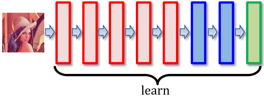
Refer to caption

(1) Jointly Trained Neural Nets
Refer to caption
(2) Fixed Neural Nets
Refer to caption
(3) Doubly Stochastic Kernel with Fixed Nets

Figure 3: Illustration of the neural nets structure in our experiments. The first several red layers are convolutions with max pooling layers. The following blue layers are fully connected layes. The green layer is the output layer which is multiclass logistic regression model.

For datasets (6) β€” (8), we compare with neural nets for images (β€œjointly-trained”). In order to directly compare the performance of nonlinear classifiers rather than feature learning abilities, we also use the convolution layers of a trained neural net to extract features, then apply our algorithm and a nonlinear neural net on top to learn classifiers (β€œfixed”). The structures of these neural nets in FigureΒ 3. For datasets (9) and (10), we compare with the neural net described inΒ [30] and use exactly the same input. In all the experiments, we select the batch size so that for each update, the computation resources can be utilized efficiently.

7.1 Kernel Ridge Regression

In this section, we compare our approach with alternative algorithms for kernel ridge regression on 2D synthetic dataset. The data are generated by

y=cos⁑(0.5​π​‖xβ€–2)​exp⁑(βˆ’0.1​π​‖xβ€–2)+0.1​e𝑦0.5πœ‹subscriptnormπ‘₯20.1πœ‹subscriptnormπ‘₯20.1𝑒\displaystyle y=\cos(0.5\pi\|x\|_{2})\exp(-0.1\pi\|x\|_{2})+0.1e

where x∈[βˆ’5,5]2π‘₯superscript552x\in[-5,5]^{2} and eβˆΌπ’©β€‹(0,1)similar-to𝑒𝒩01e\sim\mathcal{N}(0,1). We use Gaussian RBF kernel with kernel bandwidth ΟƒπœŽ\sigma chosen to be 0.10.10.1 times the median of pairwise distances between data points (median trick). The regularization parameter ν𝜈\nu is set to be 10βˆ’6superscript10610^{-6}. The batch size and feature block are set to be 210superscript2102^{10}.

The results are shown in FigureΒ 4. In FigureΒ 4(1), we plot the optimal functions generating the data. We justify our proof of the convergence rate in FigureΒ 4(2). The blue dotted line is a convergence rate of 1/t1𝑑1/t as a guide. f^tsubscript^𝑓𝑑\hat{f}_{t} denotes the average solution after t𝑑t-iteration, i.e., f^t​(x)=1tβ€‹βˆ‘i=1tfi​(x)subscript^𝑓𝑑π‘₯1𝑑superscriptsubscript𝑖1𝑑subscript𝑓𝑖π‘₯\hat{f}_{t}(x)=\frac{1}{t}\sum_{i=1}^{t}f_{i}(x). It could be seen that our algorithm indeed converges in the rate of O​(1/t)𝑂1𝑑O({1}/{t}). In FigureΒ 4 (3), we compare the first seven algorithms listed in the TableΒ 2 for solving the kernel ridge regression.

The comparison on synthetic dataset demonstrates the advantages of our algorithm clearly. Our algorithm achieves comparable performance with NORMA, which uses full kernel, in similar time but less memory cost. The pegasos and SDCA using 28superscript282^{8} random or NystrΓΆm features perform worse.

Refer to caption Refer to caption Refer to caption
(1) 2D Synthetic Dataset (2) Convergence Rate (3) Accuracy vs. Time
Figure 4: Experimental results for kernel ridge regression on synthetic dataset.
Refer to caption Refer to caption
(1) Posterior Mean Convergence (2) Posterior Variance Convergence
Figure 5: Experimental results for Gaussian Processes regression.

7.2 Gaussian Processes Regression

As we introduced in Section.Β (4), the mean and variance of posterior of Gaussian processes for regression problem can be formulated as solutions to some convex optimization problems. We conduct experiments on synthetic dataset for justification. Since the task is computing the posterior, we evaluate the performances by comparing the solutions to the posterior mean and variance, denoted as fg​psubscript𝑓𝑔𝑝f_{gp} and Οƒg​p2superscriptsubscriptπœŽπ‘”π‘2\sigma_{gp}^{2}, obtained by closed-formΒ (9). We select 211superscript2112^{11} data from the same model in previous section for training and 210superscript2102^{10} data for testing, so that the closed-form of posterior is tractable. We use Gaussian RBF kernel with kernel bandwidth ΟƒπœŽ\sigma chosen by median trick. The noise level Οƒ2superscript𝜎2\sigma^{2} is set to be 0.10.10.1. The batch size is set to be 646464 and feature block is set to be 512512512.

We compared the doubly stochastic algorithm with NORMA. The results are shown in FigureΒ 5. Both the doubly stochastic algorithm and NORMA converge to the posterior, and our algorithm achieves comparable performance with NORMA in approximating both the mean and variance.

7.3 Kernel Support Vector Machine

We evaluate our algorithm solving kernel SVM on three datasets (3)–(5) comparing with other several algorithms listed in TableΒ 2 using stopping criteria SC1 and SC2.
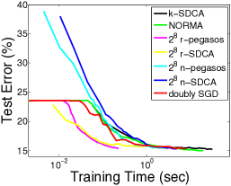
Refer to caption Refer to caption Refer to caption
SC1: (1) Adult (2) MNIST 8M 8 vs. 6 (3) Forest
Refer to caption Refer to caption Refer to caption
SC2: (4) Adult (5)MNIST 8M 8 vs. 6 (6) Forest.
Figure 6: Comparison with other kernel SVM solvers on datasets (3) – (5) with two different stopping criteria.

Adult.

We use Gaussian RBF kernel with kernel bandwidth obtained by median trick. The regularization parameter ν𝜈\nu is set to be 1/(100​n)1100𝑛1/(100n) where n𝑛n is the number of training samples. We set the batch size to be 26superscript262^{6} and feature block to be 25superscript252^{5}. After going through the whole dataset one pass, the best error rate is achieved by NORMA and k-SDCA which is 15%percent1515\% while our algorithm achieves comparable result 15.3%percent15.315.3\%. The performances are illustrated in FigureΒ 6(1). Under the same time budget, all the algorithms perform similarly in FigureΒ 6(4). The reason of flat region of r-pegasos, NORMA and the proposed method on this dataset is that Adult dataset is unbalanced. There are about 24%percent2424\% positive samples while 76%percent7676\% negative samples.

MNIST 8M 8 vs. 6.

We first reduce the dimension to 50 by PCA and use Gaussian RBF kernel with kernel bandwidth Οƒ=9.03𝜎9.03\sigma=9.03 obtained by median trick. The regularization parameter ν𝜈\nu is set to be 1/n1𝑛1/n where n𝑛n is the number of training samples. We set the batch size to be 210superscript2102^{10} and feature block to be 28superscript282^{8}. The results are shown in FigureΒ 6(2) and (5) under SC1 and SC2 respectively. Under both these two stopping criteria, our algorithm achieves the best test error 0.26%percent0.260.26\% using similar training time.

Forest.

We use Gaussian RBF kernel with kernel bandwidth obtained by median trick. The regularization parameter ν𝜈\nu is set to be 1/n1𝑛1/n where n𝑛n is the number of training samples. We set the batch size to be 210superscript2102^{10} and feature block to be 28superscript282^{8}. In FigureΒ 6(3), we shows the performances of all algorithms using SC1. NORMA and k-SDCA achieve the best error rate, which is 10%percent1010\%, while our algorithm achieves around 15%percent1515\%, but still much better than the pegasos and SDCA with 28superscript282^{8} features. In the same time budget, the proposed algorithm performs better than all the alternatives except NORMA in FigureΒ 6(6).

As seen from the performance of pegasos and SDCA on Adult and MNIST, using fewer features does not deteriorate the classification error. This might be because there are cluster structures in these two binary classification datasets. Thus, they prefer low rank approximation rather than full kernel. Different from these two datasets, in the forest dataset, algorithms with full kernel, i.e., NORMA and k-SDCA, achieve best performance. With more random features, our algorithm performs much better than pegasos and SDCA under both SC1 and SC2. Our algorithm is preferable for this scenario, i.e., huge dataset with sophisticated decision boundary. Although utilizing full kernel could achieve better performance, the computation and memory requirement for the kernel on huge dataset are costly. To learn the sophisticated boundary while still considering the computational and memory cost, we need to efficiently approximate the kernel in O​(1Ο΅)𝑂1italic-Ο΅O(\frac{1}{\epsilon}) with O​(n)𝑂𝑛O(n) random features at least. Our algorithm could handle so many random features efficiently in both computation and memory cost, while for pegasos and SDCA such operation is prohibitive.

7.4 Classification Comparisons to Convolution Neural Networks
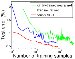
Refer to caption Refer to caption Refer to caption
(1) MNIST 8M (2) CIFAR 10 (3) ImageNet
Refer to caption Refer to caption
(4) QuantumMachine (5) MolecularSpace.
Figure 7: Comparison with Neural Networks on datasets (6) – (10).

We also compare our algorithm with the state-of-the-art neural network. In these experiments, the block size is set to be O​(104)𝑂superscript104O(10^{4}). Compared to the number of samples, O​(108)𝑂superscript108O(10^{8}), this block size is reasonable.

MNIST 8M.

In this experiment, we compare to a variant of LeNet-5Β [32], where all tanh units are replaced with rectified linear units. We also use more convolution filters and a larger fully connected layer. Specifically, the first two convolutions layers have 16 and 32 filters, respectively, and the fully connected layer contains 128 neurons. We use kernel logistic regression for the task. We extract features from the last max-pooling layer with dimension 1568, and use Gaussian RBF kernel with kernel bandwidth ΟƒπœŽ\sigma equaling to four times the median pairwise distance. The regularization parameter ν𝜈\nu is set to be 0.00050.00050.0005.

The result is shown in FigureΒ 7(1). As expected, the neural net with pre-learned features is faster to train than the jointly-trained one. However, our method is much faster compared to both methods. In addition, it achieves a lower error rate (0.5%) compared to the 0.6% error provided by the neural nets.

CIFAR 10.

In this experiment, we compare to a neural net with two convolution layers (after contrast normalization and max-pooling layers) and two local layers that achieves 11% test error222The specification is at https://code.google.com/p/cuda-convnet/ on CIFAR 10Β [28]. The features are extracted from the top max-pooling layer from a trained neural net with 2304 dimension. We use kernel logistic regression for this problem. The kernel bandwidth ΟƒπœŽ\sigma for Gaussian RBF kernel is again four times the median pairwise distance. The regularization parameter ν𝜈\nu is set to be 0.00050.00050.0005. We also perform a PCA (without centering) to reduce the dimension to 256 before feeding to our method.

The result is shown in FigureΒ 7(2). The test error for our method drops significantly faster in the earlier phase, then gradually converges to that achieved by the neural nets. Our method is able to produce the same performance within a much restricted time budget.

ImageNet.

In this experiment, we compare our algorithm with the neural nets on the ImageNet 2012 dataset, which contains 1.3 million color images from 1000 classes. Each image is of size 256 Γ—\times 256, and we randomly crop a 240 Γ—\times 240 region with random horizontal flipping. The jointly-trained neural net is Alex-netΒ [29]. The 9216 dimension features for our classifier and fixed neural net are from the last pooling layer of the jointly-trained neural net. The kernel bandwidth ΟƒπœŽ\sigma for Gaussian RBF kernel is again four times the median pairwise distance. The regularization parameter ν𝜈\nu is set to be 0.00050.00050.0005.

Test error comparisons are shown in FigureΒ 7(3). Our method achieves a test error of 44.5% by further max-voting of 10 transformations of the test set while the jointly-trained neural net arrives at 42% (without variations in color and illumination). At the same time, fixed neural net can only produce an error rate of 46% with max-voting. There may be some advantages to train the network jointly such that the layers work together to achieve a better performance. Although there is still a gap to the best performance by the jointly-trained neural net, our method comes very close with much faster convergence rate. Moreover, it achieves superior performance than the neural net with pre-learned features, both in accuracy and speed.
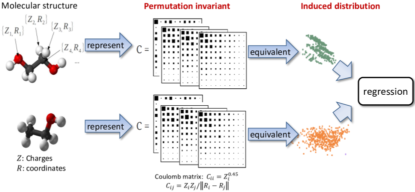
Refer to caption
Figure 8: The computational procedure for predicting molecular property from molecular structure.

7.5 Regression Comparisons to Neural Networks

We test our algorithm for kernel ridge regression with neural network proposed inΒ [30] on two large-scale real-world regression datasets, (9) and (10) in TableΒ 4. To our best knowledge, this is the first comparison between kernel ridge regression and neural network on the dataset MolecularSpace.

QuantumMachine.

In this experiment, we use the same binary representations converted based on random Coulomb matrices as inΒ [30]. We first generate a set of randomly sorted coulomb matrices for each molecule. And then, we break each dimension of the Coulomb matrix apart into steps and convert them to the binary predicates. Predictions are made by taking average of all prediction made on various Coulomb matrices of the same molecule. The procedure is illustrated in Figure.Β 8. For this experiment, 40 sets of randomly permuted matrices are generated for each training example and 20 for each test example. We use Gaussian kernel with kernel bandwidth Οƒ=60𝜎60\sigma=60 obtained by median trick. The batch size is set to be 500005000050000 and the feature block is 211superscript2112^{11}. The total dimension of random features is 220superscript2202^{20}.

The results are shown in FigureΒ 7(4). In QuantumMachine dataset, our method achieves Mean Absolute Error (MAE) of 2.972.972.97 kcal/mole, outperforming neural nets results, 3.513.513.51 kcal/mole. Note that this result is already close to the 111 kcal/mole required for chemical accuracy.

MolecularSpace.

In this experiment, the task is to predict the power conversion efficiency (PCE) of the molecule. This dataset of 2.3 million molecular motifs is obtained from the Clean Energy Project Database. We use the same feature representation as for β€œQuantumMachine” datasetΒ [30]. We set the kernel bandwidth of Gaussian RBF kernel to be 290290290 by median trick. The batch size is set to be 250002500025000 and the feature block is 211superscript2112^{11}. The total dimension of random features is 220superscript2202^{20}.

The results are shown in Figure Β 7(5). It can be seen that our method is comparable with neural network on this 2.3 million dataset.

8 Discussion

Our work contributes towards making kernel methods scalable for large-scale datasets. Specifically, by introducing artificial randomness associated with kernels besides the random data samples, we propose doubly stochastic functional gradient for kernel machines which makes the kernel machines efficient in both computation and memory requirement. Our algorithm successfully reduces the memory requirement of kernel machines from O​(d​n)𝑂𝑑𝑛O(dn) to O​(n)𝑂𝑛O(n). Meanwhile, we also show that our algorithm achieves the optimal rate of convergence, O​(1/t)𝑂1𝑑O(1/t), for strongly convex stochastic optimization. We compare our algorithm on both classification and regression problems with the state-of-the-art neural networks as well as some other competing algorithms for kernel methods on several large-scale datasets. With our efficient algorithm, kernel methods could perform comparable to sophisticated-designed neural network empirically.

The theoretical analysis, which provides the rate of convergence independent to the dimension, is also highly non-trivial. It twists martingale techniques and the vanilla analysis for stochastic gradient descent and provides a new perspective for analyzing optimization in infinite-dimensional spaces, which could be of independent interest. It should be pointed out that although we applied the algorithm to many kernel machines even with non-smooth loss functions, our current proof relies on the Lipschitz smoothness of the loss function. Extending the guarantee to non-smooth loss function will be one interesting future work.

Another key property of our method is its simplicity and ease of implementation which makes it versatile and easy to be extened in various aspects. It is straightforward to replace the sampling strategy for random features with FastfoodΒ [7] which enjoys the efficient computational cost, or Quasi-Monte Carlo samplingΒ [43], data-dependent samplingΒ [47] which enjoys faster convergence rate with fewer generated features. Meanwhile, by back-propogation trick, we could refine the random features by adapting their weights for better performanceΒ [36].

Acknowledgement

M.B. is supported in part by NSF grant CCF-1101283, AFOSR grant FA9550-09-1-0538, a Microsoft Faculty Fellowship, and a Raytheon Faculty Fellowship. L.S. is supported in part by NSF IIS-1116886, NSF/NIH BIGDATA 1R01GM108341, NSF CAREER IIS-1350983, and a Raytheon Faculty Fellowship.

References

  • [1] A.Β J. Smola and B.Β SchΓΆlkopf. Sparse greedy matrix approximation for machine learning. In ICML, pages 911–918, San Francisco, 2000. Morgan Kaufmann Publishers.
  • [2] C.Β K.Β I. Williams and M.Β Seeger. Using the Nystrom method to speed up kernel machines. In T.Β G. Dietterich, S.Β Becker, and Z.Β Ghahramani, editors, NIPS, 2000.
  • [3] S.Β Fine and K.Β Scheinberg. Efficient SVM training using low-rank kernel representations. JMLR, 2:243–264, 2001.
  • [4] P.Β Drineas and M.Β Mahoney. On the nystrβ€…om method for approximating a gram matrix for improved kernel-based learning. JMLR, 6:2153–2175, 2005.
  • [5] Corinna Cortes, Mehryar Mohri, and Ameet Talwalkar. On the impact of kernel approximation on learning accuracy. In AISTATS, pages 113–120, 2010.
  • [6] A.Β Rahimi and B.Β Recht. Random features for large-scale kernel machines. In J.C. Platt, D.Β Koller, Y.Β Singer, and S.Β Roweis, editors, NIPS. MIT Press, Cambridge, MA, 2008.
  • [7] Q.V. Le, T.Β Sarlos, and A.Β J. Smola. Fastfood β€” computing hilbert space expansions in loglinear time. In ICML, 2013.
  • [8] Ali Rahimi and Benjamin Recht. Weighted sums of random kitchen sinks: Replacing minimization with randomization in learning. In NIPS, 2009.
  • [9] David Lopez-Paz, Suvrit Sra, A.Β J. Smola, Zoubin Ghahramani, and Bernhard SchΓΆlkopf. Randomized nonlinear component analysis. In ICML, 2014.
  • [10] JohnΒ C. Platt. Sequential minimal optimization: A fast algorithm for training support vector machines. Technical Report MSR-TR-98-14, Microsoft Research, 1998.
  • [11] T.Β Joachims. Making large-scale SVM learning practical. In B.Β SchΓΆlkopf, C.Β J.Β C. Burges, and A.Β J. Smola, editors, Advances in Kernel Methods — Support Vector Learning, pages 169–184, Cambridge, MA, 1999. MIT Press.
  • [12] Shai Shalev-Shwartz and Tong Zhang. Stochastic dual coordinate ascent methods for regularized loss. JMLR, 14(1):567–599, 2013.
  • [13] J.Β Kivinen, A.Β J. Smola, and R.Β C. Williamson. Online learning with kernels. IEEE Transactions on Signal Processing, 52(8), Aug 2004.
  • [14] S.Β S. Keerthi and D.Β DeCoste. A modified finite Newton method for fast solution of large scale linear SVMs. J. Mach. Learn. Res., 6:341–361, 2005.
  • [15] N.Β Ratliff and J.Β Bagnell. Kernel conjugate gradient for fast kernel machines. In IJCAI, volumeΒ 20, January 2007.
  • [16] A.Β Nemirovski, A.Β Juditsky, G.Β Lan, and A.Β Shapiro. Robust stochastic approximation approach to stochastic programming. SIAM J. on Optimization, 19(4):1574–1609, January 2009.
  • [17] A.Β Devinatz. Integral representation of pd functions. Trans. AMS, 74(1):56–77, 1953.
  • [18] M.Β Hein and O.Β Bousquet. Kernels, associated structures, and generalizations. Technical Report 127, Max Planck Institute for Biological Cybernetics, 2004.
  • [19] H.Β Wendland. Scattered Data Approximation. Cambridge University Press, Cambridge, UK, 2005.
  • [20] Bernhard SchΓΆlkopf and A.Β J. Smola. Learning with Kernels. MIT Press, Cambridge, MA, 2002.
  • [21] N.Β Pham and R.Β Pagh. Fast and scalable polynomial kernels via explicit feature maps. In KDD. ACM, 2013.
  • [22] K.-R. MΓΌller, A.Β J. Smola, G.Β RΓ€tsch, B.Β SchΓΆlkopf, J.Β Kohlmorgen, and V.Β Vapnik. Predicting time series with support vector machines. In W.Β Gerstner, A.Β Germond, M.Β Hasler, and J.-D. Nicoud, editors, Artificial Neural Networks ICANN’97, volume 1327 of Lecture Notes in Comput. Sci., pages 999–1004, Berlin, 1997. Springer-Verlag.
  • [23] B.Β SchΓΆlkopf, J.Β Platt, J.Β Shawe-Taylor, A.Β J. Smola, and R.Β C. Williamson. Estimating the support of a high-dimensional distribution. Neural Computation, 13(7):1443–1471, 2001.
  • [24] X.L. Nguyen, M.Β Wainwright, and M.Β Jordan. Estimating divergence functionals and the likelihood ratio by penalized convex risk minimization. In Advances in Neural Information Processing Systems 20, pages 1089–1096. MIT Press, Cambridge, MA, 2008.
  • [25] AlexΒ J Smola, LeΒ Song, and ChoonΒ H Teo. Relative novelty detection. In International Conference on Artificial Intelligence and Statistics, pages 536–543, 2009.
  • [26] Shai Shalev-Shwartz, Yoram Singer, and Nathan Srebro. Pegasos: Primal estimated sub-gradient solver for SVM. In ICML, 2007.
  • [27] G.Β Loosli, S.Β Canu, and L.Β Bottou. Training invariant support vector machines with selective sampling. In L.Β Bottou, O.Β Chapelle, D.Β DeCoste, and J.Β Weston, editors, Large Scale Kernel Machines, pages 301–320. MIT Press, 2007.
  • [28] A.Β Krizhevsky. Learning multiple layers of features from tiny images. Technical report, University of Toronto, 2009.
  • [29] A.Β Krizhevsky, I.Β Sutskever, and G.Β Hinton. Imagenet classification with deep convolutional neural networks. In NIPS, 2012.
  • [30] GrΓ©goire Montavon, Katja Hansen, Siamac Fazli, Matthias Rupp, Franziska Biegler, Andreas Ziehe, Alexandre Tkatchenko, Anatole von Lilienfeld, and Klaus-Robert MΓΌller. Learning invariant representations of molecules for atomization energy prediction. In NIPS, pages 449–457, 2012.
  • [31] Alexander Rakhlin, Ohad Shamir, and Karthik Sridharan. Making gradient descent optimal for strongly convex stochastic optimization. In ICML, pages 449–456, 2012.
  • [32] Y.Β LeCun, L.Β Bottou, Y.Β Bengio, and P.Β Haffner. Gradient-based learning applied to document recognition. Proceedings of the IEEE, 86(11):2278–2324, November 1998.
  • [33] Purushottam Kar and Harish Karnick. Random feature maps for dot product kernels. In NeilΒ D. Lawrence and MarkΒ A. Girolami, editors, AISTATS-12, volumeΒ 22, pages 583–591, 2012.
  • [34] Andrea Vedaldi and Andrew Zisserman. Efficient additive kernels via explicit feature maps. IEEE Trans. Pattern Anal. Mach. Intell., 34(3):480–492, 2012.
  • [35] Jiyan Yang, Vikas Sindhwani, Quanfu Fan, Haim Avron, and MichaelΒ W. Mahoney. Random laplace feature maps for semigroup kernels on histograms. In CVPR, 2014.
  • [36] Zichao Yang, Marcin Moczulski, Misha Denil, Nando deΒ Freitas, AlexanderΒ J. Smola, LeΒ Song, and Ziyu Wang. Deep fried convnets. CoRR, abs/1412.7149, 2014d. URL http://arxiv.org/abs/1412.7149.
  • [37] Rie Johnson and Tong Zhang. Accelerating stochastic gradient descent using predictive variance reduction. In NIPS, pages 315–323, 2013.
  • [38] CongΒ D. Dang and Guanghui Lan. Stochastic block mirror descent methods for nonsmooth and stochastic optimization. Technical report, University of Florida, 2013.
  • [39] Yurii Nesterov. Efficiency of coordinate descent methods on huge-scale optimization problems. SIAM Journal on Optimization, 22(2):341–362, 2012.
  • [40] Andrew Cotter, Shai Shalev-Shwartz, and Nati Srebro. Learning optimally sparse support vector machines. In Proceedings of the 30th International Conference on Machine Learning, ICML 2013, Atlanta, GA, USA, 16-21 June 2013, pages 266–274, 2013.
  • [41] A.Β Agarwal, S.Β Kakade, N.Β Karampatziakis, L.Β Song, and G.Β Valiant. Least squares revisited: Scalable approaches for multi-class prediction. In International Conference on Machine Learning (ICML), 2014.
  • [42] Tianbao Yang, Rong Jin, and Shenghuo Zhu. On data preconditioning for regularized loss minimization. CoRR, 2014.
  • [43] Jiyan Yang, Vikas Sindhwani, Haim Avron, and MichaelΒ W. Mahoney. Quasi-monte carlo feature maps for shift-invariant kernels. In Proceedings of the 31th International Conference on Machine Learning, ICML 2014, Beijing, China, 21-26 June 2014, pages 485–493, 2014.
  • [44] Gaurav Pandey and Ambedkar Dukkipati. Learning by stretching deep networks. In Proceedings of the 31th International Conference on Machine Learning, ICML 2014, Beijing, China, 21-26 June 2014, pages 485–493, 2014.
  • [45] Youngmin Cho and LawrenceΒ K. Saul. Kernel methods for deep learning. In Y.Β Bengio, D.Β Schuurmans, J.D. Lafferty, C.K.I. Williams, and A.Β Culotta, editors, Advances in Neural Information Processing Systems 22, pages 342–350, 2009.
  • [46] C.Β E. Rasmussen and C.Β K.Β I. Williams. Gaussian Processes for Machine Learning. MIT Press, Cambridge, MA, 2006.
  • [47] FrancisΒ R. Bach. On the equivalence between quadrature rules and random features. CoRR, abs/1502.06800, 2015. URL http://arxiv.org/abs/1502.06800.

Appendix

Appendix A Convergence Rate

We first provide specific bounds and detailed proofs for the two error terms appeared in Theorem 4 and Theorem 5.

A.1 Error due to random features

Lemma 7

We have

  1. (i)

    For any xβˆˆπ’³π‘₯𝒳x\in\mathcal{X}, π”Όπ’Ÿt,𝝎t​[|ft+1​(x)βˆ’ht+1​(x)|2]β©½B1,t+12:=4​M2​(ΞΊ+Ο•)2β€‹βˆ‘i=1t|ati|2.subscript𝔼superscriptπ’Ÿπ‘‘superscriptπŽπ‘‘delimited-[]superscriptsubscript𝑓𝑑1π‘₯subscriptβ„Žπ‘‘1π‘₯2subscriptsuperscript𝐡21𝑑1assign4superscript𝑀2superscriptπœ…italic-Ο•2superscriptsubscript𝑖1𝑑superscriptsuperscriptsubscriptπ‘Žπ‘‘π‘–2\mathbb{E}_{\mathcal{D}^{t},\bm{\omega}^{t}}[|f_{t+1}(x)-h_{t+1}(x)|^{2}]\leqslant B^{2}_{1,t+1}:=4M^{2}(\kappa+\phi)^{2}\sum_{i=1}^{t}|a_{t}^{i}|^{2}.

  2. (ii)

    For any xβˆˆπ’³π‘₯𝒳x\in\mathcal{X}, with probability at least 1βˆ’Ξ΄1𝛿1-\delta over (π’Ÿt,𝝎t)superscriptπ’Ÿπ‘‘superscriptπŽπ‘‘(\mathcal{D}^{t},\bm{\omega}^{t}),

    |ft+1​(x)βˆ’ht+1​(x)|2β©½B2,t+12:=2​M2​(ΞΊ+Ο•)2​ln⁑(2Ξ΄)β€‹βˆ‘i=1t|ati|2superscriptsubscript𝑓𝑑1π‘₯subscriptβ„Žπ‘‘1π‘₯2subscriptsuperscript𝐡22𝑑1assign2superscript𝑀2superscriptπœ…italic-Ο•22𝛿superscriptsubscript𝑖1𝑑superscriptsubscriptsuperscriptπ‘Žπ‘–π‘‘2|f_{t+1}(x)-h_{t+1}(x)|^{2}\leqslant B^{2}_{2,t+1}:=2M^{2}(\kappa+\phi)^{2}\ln\left(\frac{2}{\delta}\right)\sum_{i=1}^{t}|a^{i}_{t}|^{2}

ProofΒ  Let Vi​(x)=Vi​(x;π’Ÿi,𝝎i):=ati​(ΞΆi​(x)βˆ’ΞΎi​(x))subscript𝑉𝑖π‘₯subscript𝑉𝑖π‘₯superscriptπ’Ÿπ‘–superscriptπŽπ‘–assignsuperscriptsubscriptπ‘Žπ‘‘π‘–subscriptπœπ‘–π‘₯subscriptπœ‰π‘–π‘₯V_{i}(x)=V_{i}(x;\mathcal{D}^{i},\bm{\omega}^{i}):=a_{t}^{i}\left(\zeta_{i}(x)-\xi_{i}(x)\right). Since Vi​(x)subscript𝑉𝑖π‘₯V_{i}(x) is a function of (π’Ÿi,𝝎i)superscriptπ’Ÿπ‘–superscriptπŽπ‘–(\mathcal{D}^{i},\bm{\omega}^{i}) and

π”Όπ’Ÿi,𝝎i​[Vi​(x)|𝝎iβˆ’1]=atiβ€‹π”Όπ’Ÿi,𝝎i​[ΞΆi​(x)βˆ’ΞΎi​(x)|𝝎iβˆ’1]=atiβ€‹π”Όπ’Ÿi,𝝎iβˆ’1​[𝔼ωi​[ΞΆi​(x)βˆ’ΞΎi​(x)|𝝎iβˆ’1]]=0,subscript𝔼superscriptπ’Ÿπ‘–superscriptπŽπ‘–delimited-[]conditionalsubscript𝑉𝑖π‘₯superscriptπŽπ‘–1superscriptsubscriptπ‘Žπ‘‘π‘–subscript𝔼superscriptπ’Ÿπ‘–superscriptπŽπ‘–delimited-[]subscriptπœπ‘–π‘₯conditionalsubscriptπœ‰π‘–π‘₯superscriptπŽπ‘–1superscriptsubscriptπ‘Žπ‘‘π‘–subscript𝔼superscriptπ’Ÿπ‘–superscriptπŽπ‘–1delimited-[]subscript𝔼superscriptπœ”π‘–delimited-[]subscriptπœπ‘–π‘₯conditionalsubscriptπœ‰π‘–π‘₯superscriptπŽπ‘–10\mathbb{E}_{\mathcal{D}^{i},\bm{\omega}^{i}}\left[V_{i}(x)|\bm{\omega}^{i-1}\right]=a_{t}^{i}\mathbb{E}_{\mathcal{D}^{i},\bm{\omega}^{i}}\left[\zeta_{i}(x)-\xi_{i}(x)|\bm{\omega}^{i-1}\right]=a_{t}^{i}\mathbb{E}_{\mathcal{D}^{i},\bm{\omega}^{i-1}}\left[\mathbb{E}_{\omega^{i}}\left[\zeta_{i}(x)-\xi_{i}(x)|\bm{\omega}^{i-1}\right]\right]=0,

we have that {Vi​(x)}subscript𝑉𝑖π‘₯\left\{V_{i}(x)\right\} is a martingal difference sequence. Further note that

|Vi​(x)|β©½ci=2​M​(Ο•+ΞΊ)​|ati|.subscript𝑉𝑖π‘₯subscript𝑐𝑖2𝑀italic-Ο•πœ…superscriptsubscriptπ‘Žπ‘‘π‘–|V_{i}(x)|\leqslant c_{i}=2M(\phi+\kappa)|a_{t}^{i}|.

Then by Azuma’s Inequality, for any Ο΅>0italic-Ο΅0\epsilon>0,

Prπ’Ÿt,𝝎t⁑{|βˆ‘i=1tVi​(x)|β©ΎΟ΅}β©½2​exp⁑{βˆ’2​ϡ2βˆ‘i=1tci2}subscriptPrsuperscriptπ’Ÿπ‘‘superscriptπŽπ‘‘superscriptsubscript𝑖1𝑑subscript𝑉𝑖π‘₯italic-Ο΅22superscriptitalic-Ο΅2superscriptsubscript𝑖1𝑑superscriptsubscript𝑐𝑖2\Pr_{\mathcal{D}^{t},\bm{\omega}^{t}}\left\{|\sum_{i=1}^{t}V_{i}(x)|\geqslant\epsilon\right\}\leqslant 2\exp\left\{-\frac{2\epsilon^{2}}{\sum_{i=1}^{t}c_{i}^{2}}\right\}

which is equivalent as

Prπ’Ÿt,𝝎t⁑{(βˆ‘i=1tVi​(x))2β©Ύln⁑(2/Ξ΄)β€‹βˆ‘i=1tci2/2}β©½Ξ΄.subscriptPrsuperscriptπ’Ÿπ‘‘superscriptπŽπ‘‘superscriptsuperscriptsubscript𝑖1𝑑subscript𝑉𝑖π‘₯22𝛿superscriptsubscript𝑖1𝑑superscriptsubscript𝑐𝑖22𝛿\Pr_{\mathcal{D}^{t},\bm{\omega}^{t}}\left\{\left(\sum_{i=1}^{t}V_{i}(x)\right)^{2}\geqslant\ln(2/\delta)\sum_{i=1}^{t}c_{i}^{2}/2\right\}\leqslant\delta.

Moreover,

π”Όπ’Ÿt,𝝎t​[(βˆ‘i=1tVi​(x))2]subscript𝔼superscriptπ’Ÿπ‘‘superscriptπŽπ‘‘delimited-[]superscriptsuperscriptsubscript𝑖1𝑑subscript𝑉𝑖π‘₯2\displaystyle\mathbb{E}_{\mathcal{D}^{t},\bm{\omega}^{t}}\left[\left(\sum_{i=1}^{t}V_{i}(x)\right)^{2}\right] =∫0∞Prπ’Ÿt,𝝎t⁑{(βˆ‘i=1tVi​(x))2β©ΎΟ΅}​𝑑ϡ=∫0∞2​exp⁑{βˆ’2β€‹Ο΅βˆ‘i=1tci2}​𝑑ϡ=βˆ‘i=1tci2absentsuperscriptsubscript0subscriptPrsuperscriptπ’Ÿπ‘‘superscriptπŽπ‘‘superscriptsuperscriptsubscript𝑖1𝑑subscript𝑉𝑖π‘₯2italic-Ο΅differential-ditalic-Ο΅superscriptsubscript022italic-Ο΅superscriptsubscript𝑖1𝑑superscriptsubscript𝑐𝑖2differential-ditalic-Ο΅superscriptsubscript𝑖1𝑑superscriptsubscript𝑐𝑖2\displaystyle=\int_{0}^{\infty}\Pr_{\mathcal{D}^{t},\bm{\omega}^{t}}\left\{\left(\sum_{i=1}^{t}V_{i}(x)\right)^{2}\geqslant\epsilon\right\}d\epsilon=\int_{0}^{\infty}2\exp\left\{-\frac{2\epsilon}{\sum_{i=1}^{t}c_{i}^{2}}\right\}d\epsilon=\sum_{i=1}^{t}c_{i}^{2}

Since ft+1​(x)βˆ’ht+1​(x)=βˆ‘i=1tVi​(x)subscript𝑓𝑑1π‘₯subscriptβ„Žπ‘‘1π‘₯superscriptsubscript𝑖1𝑑subscript𝑉𝑖π‘₯f_{t+1}(x)-h_{t+1}(x)=\sum_{i=1}^{t}V_{i}(x), we immediately obtain the two parts of the lemma. Β 

Lemma 8

Suppose Ξ³i=ΞΈi​(1β©½iβ©½t)subscriptπ›Ύπ‘–πœƒπ‘–1𝑖𝑑\gamma_{i}=\frac{\theta}{i}(1\leqslant i\leqslant t) and ΞΈβ€‹Ξ½βˆˆ(1,2)βˆͺβ„€+πœƒπœˆ12subscriptβ„€\theta\nu\in(1,2)\cup\mathbb{Z}_{+}. Then we have

  1. (1)

    |ati|β©½ΞΈtsubscriptsuperscriptπ‘Žπ‘–π‘‘πœƒπ‘‘|a^{i}_{t}|\leqslant\frac{\theta}{t}. Consequently, βˆ‘i=1t(ati)2β©½ΞΈ2t.superscriptsubscript𝑖1𝑑superscriptsubscriptsuperscriptπ‘Žπ‘–π‘‘2superscriptπœƒ2𝑑\sum_{i=1}^{t}(a^{i}_{t})^{2}\leqslant\frac{\theta^{2}}{t}.

  2. (2)

    βˆ‘i=1tΞ³i​|ati|β©½{ΞΈ2​(ln⁑(t)+1)t,ifΒ β€‹ΞΈβ€‹Ξ½βˆˆ[1,2),ΞΈ2t,ifΒ β€‹ΞΈβ€‹Ξ½βˆˆ[2,+∞)βˆ©β„€+superscriptsubscript𝑖1𝑑subscript𝛾𝑖superscriptsubscriptπ‘Žπ‘‘π‘–casessuperscriptπœƒ2𝑑1𝑑ifΒ πœƒπœˆ12superscriptπœƒ2𝑑ifΒ πœƒπœˆ2subscriptβ„€\sum_{i=1}^{t}\gamma_{i}|a_{t}^{i}|\leqslant\left\{\begin{array}[]{ll}\frac{\theta^{2}(\ln(t)+1)}{t},&\text{if }\theta\nu\in[1,2),\\ \frac{\theta^{2}}{t},&\text{if }\theta\nu\in[2,+\infty)\cap\mathbb{Z}_{+}\end{array}\right..

ProofΒ  (1)1(1) follows by induction on i𝑖i. |att|β©½ΞΈtsuperscriptsubscriptπ‘Žπ‘‘π‘‘πœƒπ‘‘|a_{t}^{t}|\leqslant\frac{\theta}{t} is trivially true. We have

|ati|superscriptsubscriptπ‘Žπ‘‘π‘–\displaystyle|a_{t}^{i}| =|ati+1​γiΞ³i+1​(1βˆ’Ξ½β€‹Ξ³i+1)|=i+1i​|1βˆ’Ξ½β€‹ΞΈi+1|β‹…|ati+1|=|i+1βˆ’Ξ½β€‹ΞΈi|β‹…|ati+1|.absentsuperscriptsubscriptπ‘Žπ‘‘π‘–1subscript𝛾𝑖subscript𝛾𝑖11𝜈subscript𝛾𝑖1⋅𝑖1𝑖1πœˆπœƒπ‘–1superscriptsubscriptπ‘Žπ‘‘π‘–1⋅𝑖1πœˆπœƒπ‘–superscriptsubscriptπ‘Žπ‘‘π‘–1\displaystyle=|a_{t}^{i+1}\frac{\gamma_{i}}{\gamma_{i+1}}(1-\nu\gamma_{i+1})|=\frac{i+1}{i}|1-\frac{\nu\theta}{i+1}|\cdot|a_{t}^{i+1}|=|\frac{i+1-\nu\theta}{i}|\cdot|a_{t}^{i+1}|.

When Ξ½β€‹ΞΈβˆˆ(1,2)πœˆπœƒ12\nu\theta\in(1,2), iβˆ’1<i+1βˆ’Ξ½β€‹ΞΈ<i𝑖1𝑖1πœˆπœƒπ‘–i-1<i+1-\nu\theta<i for any iβ©Ύ1𝑖1i\geqslant 1, so |ati|<|ati+1|β©½ΞΈtsuperscriptsubscriptπ‘Žπ‘‘π‘–superscriptsubscriptπ‘Žπ‘‘π‘–1πœƒπ‘‘|a_{t}^{i}|<|a_{t}^{i+1}|\leqslant\frac{\theta}{t}. When Ξ½β€‹ΞΈβˆˆβ„€+πœˆπœƒsubscriptβ„€\nu\theta\in\mathbb{Z}_{+}, if i>Ξ½β€‹ΞΈβˆ’1π‘–πœˆπœƒ1i>\nu\theta-1, then |ati|<|ati+1|β©½ΞΈtsuperscriptsubscriptπ‘Žπ‘‘π‘–superscriptsubscriptπ‘Žπ‘‘π‘–1πœƒπ‘‘|a_{t}^{i}|<|a_{t}^{i+1}|\leqslant\frac{\theta}{t}; if iβ©½Ξ½β€‹ΞΈβˆ’1π‘–πœˆπœƒ1i\leqslant\nu\theta-1, then |ati|=0superscriptsubscriptπ‘Žπ‘‘π‘–0|a_{t}^{i}|=0. For (2)2(2), when ΞΈβ€‹Ξ½βˆˆ[1,2)πœƒπœˆ12\theta\nu\in[1,2),

βˆ‘i=1tΞ³t​|ati|=βˆ‘i=1tΞΈ2i2β‹…i+1βˆ’ΞΈβ€‹Ξ½i+1​⋯​tβˆ’ΞΈβ€‹Ξ½tβ©½βˆ‘i=1tΞΈ2i2β‹…ii+1​⋯​tβˆ’1tβ©½βˆ‘i=1tΞΈ2i​tβ©½ΞΈ2​(ln⁑(t)+1)t.superscriptsubscript𝑖1𝑑subscript𝛾𝑑superscriptsubscriptπ‘Žπ‘‘π‘–superscriptsubscript𝑖1𝑑⋅superscriptπœƒ2superscript𝑖2𝑖1πœƒπœˆπ‘–1β‹―π‘‘πœƒπœˆπ‘‘superscriptsubscript𝑖1𝑑⋅superscriptπœƒ2superscript𝑖2𝑖𝑖1⋯𝑑1𝑑superscriptsubscript𝑖1𝑑superscriptπœƒ2𝑖𝑑superscriptπœƒ2𝑑1𝑑\sum_{i=1}^{t}\gamma_{t}|a_{t}^{i}|=\sum_{i=1}^{t}\frac{\theta^{2}}{i^{2}}\cdot\frac{i+1-\theta\nu}{i+1}\cdots\frac{t-\theta\nu}{t}\leqslant\sum_{i=1}^{t}\frac{\theta^{2}}{i^{2}}\cdot\frac{i}{i+1}\cdots\frac{t-1}{t}\leqslant\sum_{i=1}^{t}\frac{\theta^{2}}{it}\leqslant\frac{\theta^{2}(\ln(t)+1)}{t}.

When ΞΈβ€‹Ξ½βˆˆβ„€+πœƒπœˆsubscriptβ„€\theta\nu\in\mathbb{Z}_{+} and 2⩽θ​ν⩽t,2πœƒπœˆπ‘‘2\leqslant\theta\nu\leqslant t,

βˆ‘i=1tΞ³t​|ati|=βˆ‘i=2tΞΈ2i2β‹…i+1βˆ’ΞΈβ€‹Ξ½i+1​⋯​tβˆ’ΞΈβ€‹Ξ½tβ©½βˆ‘i=1tΞΈ2i2β‹…iβˆ’1i+1​⋯​tβˆ’2tβ©½βˆ‘i=2tΞΈ2​(iβˆ’1)i​t​(tβˆ’1)β©½ΞΈ2t.superscriptsubscript𝑖1𝑑subscript𝛾𝑑superscriptsubscriptπ‘Žπ‘‘π‘–superscriptsubscript𝑖2𝑑⋅superscriptπœƒ2superscript𝑖2𝑖1πœƒπœˆπ‘–1β‹―π‘‘πœƒπœˆπ‘‘superscriptsubscript𝑖1𝑑⋅superscriptπœƒ2superscript𝑖2𝑖1𝑖1⋯𝑑2𝑑superscriptsubscript𝑖2𝑑superscriptπœƒ2𝑖1𝑖𝑑𝑑1superscriptπœƒ2𝑑\sum_{i=1}^{t}\gamma_{t}|a_{t}^{i}|=\sum_{i=2}^{t}\frac{\theta^{2}}{i^{2}}\cdot\frac{i+1-\theta\nu}{i+1}\cdots\frac{t-\theta\nu}{t}\leqslant\sum_{i=1}^{t}\frac{\theta^{2}}{i^{2}}\cdot\frac{i-1}{i+1}\cdots\frac{t-2}{t}\leqslant\sum_{i=2}^{t}\frac{\theta^{2}(i-1)}{it(t-1)}\leqslant\frac{\theta^{2}}{t}.

Β 

A.2 Error due to random data

Lemma 9

Assume l′​(u,y)superscript𝑙′𝑒𝑦l^{\prime}(u,y) is L𝐿L-Lipschitz continous in terms of uβˆˆβ„π‘’β„u\in\mathbb{R}. Let fβˆ—subscript𝑓f_{*} be the optimal solution to our target problem. Then

  1. (i)

    If we set Ξ³t=ΞΈtsubscriptπ›Ύπ‘‘πœƒπ‘‘\gamma_{t}=\frac{\theta}{t} with ΞΈπœƒ\theta such that ΞΈβ€‹Ξ½βˆˆ(1,2)βˆͺβ„€+πœƒπœˆ12subscriptβ„€\theta\nu\in(1,2)\cup\mathbb{Z}_{+}, then

    π”Όπ’Ÿt,𝝎t​[β€–ht+1βˆ’fβˆ—β€–β„‹2]β©½Q12t,subscript𝔼superscriptπ’Ÿπ‘‘superscriptπŽπ‘‘delimited-[]subscriptsuperscriptnormsubscriptβ„Žπ‘‘1subscriptπ‘“βˆ—2β„‹superscriptsubscript𝑄12𝑑\mathbb{E}_{\mathcal{D}^{t},\bm{\omega}^{t}}\left[\left\|h_{t+1}-f_{\ast}\right\|^{2}_{\mathcal{H}}\right]\leqslant\frac{Q_{1}^{2}}{t},

    where

    Q1=max⁑{β€–fβˆ—β€–β„‹,Q0+Q02+(2β€‹ΞΈβ€‹Ξ½βˆ’1)​(1+θ​ν)2​θ2​κ​M22β€‹Ξ½β€‹ΞΈβˆ’1},Q0=2​2​κ1/2​(ΞΊ+Ο•)​L​M​θ2.formulae-sequencesubscript𝑄1subscriptnormsubscriptπ‘“βˆ—β„‹subscript𝑄0superscriptsubscript𝑄022πœƒπœˆ1superscript1πœƒπœˆ2superscriptπœƒ2πœ…superscript𝑀22πœˆπœƒ1subscript𝑄022superscriptπœ…12πœ…italic-ϕ𝐿𝑀superscriptπœƒ2Q_{1}=\max\left\{\left\|f_{\ast}\right\|_{\mathcal{H}},\frac{Q_{0}+\sqrt{Q_{0}^{2}+(2\theta\nu-1)(1+\theta\nu)^{2}\theta^{2}\kappa M^{2}}}{2\nu\theta-1}\right\},Q_{0}=2\sqrt{2}\kappa^{1/2}(\kappa+\phi)LM\theta^{2}.

    Particularly, if θ​ν=1πœƒπœˆ1\theta\nu=1, we have Q1β©½max⁑{β€–fβˆ—β€–β„‹,4​2​((ΞΊ+Ο•)​L+Ξ½)β‹…ΞΊ1/2​MΞ½2}subscript𝑄1subscriptnormsubscriptπ‘“βˆ—β„‹β‹…42πœ…italic-Ο•πΏπœˆsuperscriptπœ…12𝑀superscript𝜈2Q_{1}\leqslant\max\left\{\left\|f_{\ast}\right\|_{\mathcal{H}},4\sqrt{2}((\kappa+\phi)L+\nu)\cdot\frac{\kappa^{1/2}M}{\nu^{2}}\right\}.

  2. (ii)

    If we set Ξ³t=ΞΈtsubscriptπ›Ύπ‘‘πœƒπ‘‘\gamma_{t}=\frac{\theta}{t} with ΞΈπœƒ\theta such that ΞΈβ€‹Ξ½βˆˆβ„€+πœƒπœˆsubscriptβ„€\theta\nu\in\mathbb{Z}_{+} and tβ©ΎΞΈβ€‹Ξ½π‘‘πœƒπœˆt\geqslant\theta\nu, then with probability at least 1βˆ’2​δ12𝛿1-2\delta over (π’Ÿt,𝝎t)superscriptπ’Ÿπ‘‘superscriptπŽπ‘‘(\mathcal{D}^{t},\bm{\omega}^{t}),

    β€–ht+1βˆ’fβˆ—β€–β„‹2β©½Q22​ln⁑(2​t/Ξ΄)​ln⁑(t)t.subscriptsuperscriptnormsubscriptβ„Žπ‘‘1subscriptπ‘“βˆ—2β„‹superscriptsubscript𝑄222𝑑𝛿𝑑𝑑\left\|h_{t+1}-f_{\ast}\right\|^{2}_{\mathcal{H}}\leqslant Q_{2}^{2}\frac{\ln(2t/\delta)\ln(t)}{t}.

    where

    Q2=max⁑{β€–fβˆ—β€–β„‹,Q0+Q02+κ​M2​(1+θ​ν)2​(ΞΈ2+16​θ/Ξ½)},Q0=4​2​κ1/2​M​θ​(8+(ΞΊ+Ο•)​θ​L).formulae-sequencesubscript𝑄2subscriptnormsubscriptπ‘“βˆ—β„‹subscript𝑄0superscriptsubscript𝑄02πœ…superscript𝑀2superscript1πœƒπœˆ2superscriptπœƒ216πœƒπœˆsubscript𝑄042superscriptπœ…12π‘€πœƒ8πœ…italic-Ο•πœƒπΏQ_{2}=\max\left\{\left\|f_{\ast}\right\|_{\mathcal{H}},Q_{0}+\sqrt{Q_{0}^{2}+\kappa M^{2}(1+\theta\nu)^{2}(\theta^{2}+16\theta/\nu)}\right\},Q_{0}=4\sqrt{2}\kappa^{1/2}M\theta(8+(\kappa+\phi)\theta L).

    Particularly, if θ​ν=1πœƒπœˆ1\theta\nu=1, we have Q2β©½max⁑{β€–fβˆ—β€–β„‹,8​2​((ΞΊ+Ο•)​L+9​ν)β‹…ΞΊ1/2​MΞ½2}subscript𝑄2subscriptnormsubscriptπ‘“βˆ—β„‹β‹…82πœ…italic-ϕ𝐿9𝜈superscriptπœ…12𝑀superscript𝜈2Q_{2}\leqslant\max\left\{\left\|f_{\ast}\right\|_{\mathcal{H}},8\sqrt{2}((\kappa+\phi)L+9\nu)\cdot\frac{\kappa^{1/2}M}{\nu^{2}}\right\}.

ProofΒ  For the sake of simple notations, let us first denote the following three different gradient terms, which are

gtsubscript𝑔𝑑\displaystyle g_{t} =ΞΎt+ν​ht=l′​(ft​(xt),yt)​k​(xt,β‹…)+ν​ht,absentsubscriptπœ‰π‘‘πœˆsubscriptβ„Žπ‘‘superscript𝑙′subscript𝑓𝑑subscriptπ‘₯𝑑subscriptπ‘¦π‘‘π‘˜subscriptπ‘₯π‘‘β‹…πœˆsubscriptβ„Žπ‘‘\displaystyle=\xi_{t}+\nu h_{t}=l^{\prime}(f_{t}(x_{t}),y_{t})k(x_{t},\cdot)+\nu h_{t},
g^tsubscript^𝑔𝑑\displaystyle\hat{g}_{t} =ΞΎ^t+ν​ht=l′​(ht​(xt),yt)​k​(xt,β‹…)+ν​ht,absentsubscript^πœ‰π‘‘πœˆsubscriptβ„Žπ‘‘superscript𝑙′subscriptβ„Žπ‘‘subscriptπ‘₯𝑑subscriptπ‘¦π‘‘π‘˜subscriptπ‘₯π‘‘β‹…πœˆsubscriptβ„Žπ‘‘\displaystyle=\hat{\xi}_{t}+\nu h_{t}=l^{\prime}(h_{t}(x_{t}),y_{t})k(x_{t},\cdot)+\nu h_{t},
gΒ―tsubscript¯𝑔𝑑\displaystyle\bar{g}_{t} =π”Όπ’Ÿt​[g^t]=π”Όπ’Ÿt​[l′​(ht​(xt),yt)​k​(xt,β‹…)]+ν​ht.absentsubscript𝔼subscriptπ’Ÿπ‘‘delimited-[]subscript^𝑔𝑑subscript𝔼subscriptπ’Ÿπ‘‘delimited-[]superscript𝑙′subscriptβ„Žπ‘‘subscriptπ‘₯𝑑subscriptπ‘¦π‘‘π‘˜subscriptπ‘₯π‘‘β‹…πœˆsubscriptβ„Žπ‘‘\displaystyle=\mathbb{E}_{\mathcal{D}_{t}}\left[\hat{g}_{t}\right]=\mathbb{E}_{\mathcal{D}_{t}}\left[l^{\prime}(h_{t}(x_{t}),y_{t})k(x_{t},\cdot)\right]+\nu h_{t}.

Note that by our previous definition, we have ht+1=htβˆ’Ξ³t​gt,βˆ€tβ©Ύ1formulae-sequencesubscriptβ„Žπ‘‘1subscriptβ„Žπ‘‘subscript𝛾𝑑subscript𝑔𝑑for-all𝑑1h_{t+1}=h_{t}-\gamma_{t}g_{t},\forall t\geqslant 1.

Denote At=β€–htβˆ’fβˆ—β€–β„‹2subscript𝐴𝑑subscriptsuperscriptnormsubscriptβ„Žπ‘‘subscriptπ‘“βˆ—2β„‹A_{t}=\left\|h_{t}-f_{\ast}\right\|^{2}_{\mathcal{H}}. Then we have

At+1subscript𝐴𝑑1\displaystyle A_{t+1} =\displaystyle= β€–htβˆ’fβˆ—βˆ’Ξ³t​gtβ€–β„‹2superscriptsubscriptnormsubscriptβ„Žπ‘‘subscriptπ‘“βˆ—subscript𝛾𝑑subscript𝑔𝑑ℋ2\displaystyle\left\|h_{t}-f_{\ast}-\gamma_{t}g_{t}\right\|_{\mathcal{H}}^{2}
=\displaystyle= At+Ξ³t2​‖gtβ€–β„‹2βˆ’2​γtβ€‹βŸ¨htβˆ’fβˆ—,gtβŸ©β„‹subscript𝐴𝑑superscriptsubscript𝛾𝑑2subscriptsuperscriptnormsubscript𝑔𝑑2β„‹2subscript𝛾𝑑subscriptsubscriptβ„Žπ‘‘subscriptπ‘“βˆ—subscript𝑔𝑑ℋ\displaystyle A_{t}+\gamma_{t}^{2}\left\|g_{t}\right\|^{2}_{\mathcal{H}}-2\gamma_{t}\langle h_{t}-f_{\ast},g_{t}\rangle_{\mathcal{H}}
=\displaystyle= At+Ξ³t2​‖gtβ€–β„‹2βˆ’2​γtβ€‹βŸ¨htβˆ’fβˆ—,gΒ―tβŸ©β„‹+2​γtβ€‹βŸ¨htβˆ’fβˆ—,gΒ―tβˆ’g^tβŸ©β„‹+2​γtβ€‹βŸ¨htβˆ’fβˆ—,g^tβˆ’gtβŸ©β„‹subscript𝐴𝑑superscriptsubscript𝛾𝑑2subscriptsuperscriptnormsubscript𝑔𝑑2β„‹2subscript𝛾𝑑subscriptsubscriptβ„Žπ‘‘subscriptπ‘“βˆ—subscript¯𝑔𝑑ℋ2subscript𝛾𝑑subscriptsubscriptβ„Žπ‘‘subscriptπ‘“βˆ—subscript¯𝑔𝑑subscript^𝑔𝑑ℋ2subscript𝛾𝑑subscriptsubscriptβ„Žπ‘‘subscriptπ‘“βˆ—subscript^𝑔𝑑subscript𝑔𝑑ℋ\displaystyle A_{t}+\gamma_{t}^{2}\left\|g_{t}\right\|^{2}_{\mathcal{H}}-2\gamma_{t}\langle h_{t}-f_{\ast},\bar{g}_{t}\rangle_{\mathcal{H}}+2\gamma_{t}\langle h_{t}-f_{\ast},\bar{g}_{t}-\hat{g}_{t}\rangle_{\mathcal{H}}+2\gamma_{t}\langle h_{t}-f_{\ast},\hat{g}_{t}-g_{t}\rangle_{\mathcal{H}}

Because of the strongly convexity ofΒ (1) and optimality condition, we have

⟨htβˆ’fβˆ—,gΒ―tβŸ©β„‹β©ΎΞ½β€‹β€–htβˆ’fβˆ—β€–β„‹2subscriptsubscriptβ„Žπ‘‘subscriptπ‘“βˆ—subscriptΒ―π‘”π‘‘β„‹πœˆsubscriptsuperscriptnormsubscriptβ„Žπ‘‘subscriptπ‘“βˆ—2β„‹\displaystyle\langle h_{t}-f_{\ast},\bar{g}_{t}\rangle_{\mathcal{H}}\geqslant\nu\left\|h_{t}-f_{\ast}\right\|^{2}_{\mathcal{H}}

Hence, we have

At+1β©½(1βˆ’2​γt​ν)​At+Ξ³t2​‖gtβ€–β„‹2+2​γtβ€‹βŸ¨htβˆ’fβˆ—,gΒ―tβˆ’g^tβŸ©β„‹+2​γtβ€‹βŸ¨htβˆ’fβˆ—,g^tβˆ’gtβŸ©β„‹,βˆ€tβ©Ύ1formulae-sequencesubscript𝐴𝑑112subscriptπ›Ύπ‘‘πœˆsubscript𝐴𝑑superscriptsubscript𝛾𝑑2subscriptsuperscriptnormsubscript𝑔𝑑2β„‹2subscript𝛾𝑑subscriptsubscriptβ„Žπ‘‘subscriptπ‘“βˆ—subscript¯𝑔𝑑subscript^𝑔𝑑ℋ2subscript𝛾𝑑subscriptsubscriptβ„Žπ‘‘subscriptπ‘“βˆ—subscript^𝑔𝑑subscript𝑔𝑑ℋfor-all𝑑1A_{t+1}\leqslant(1-2\gamma_{t}\nu)A_{t}+\gamma_{t}^{2}\left\|g_{t}\right\|^{2}_{\mathcal{H}}+2\gamma_{t}\langle h_{t}-f_{\ast},\bar{g}_{t}-\hat{g}_{t}\rangle_{\mathcal{H}}+2\gamma_{t}\langle h_{t}-f_{\ast},\hat{g}_{t}-g_{t}\rangle_{\mathcal{H}},\forall t\geqslant 1 (12)

Proof for (i)𝑖(i): Let us denote β„³t=β€–gtβ€–β„‹2subscriptℳ𝑑subscriptsuperscriptnormsubscript𝑔𝑑2β„‹\mathcal{M}_{t}=\left\|g_{t}\right\|^{2}_{\mathcal{H}}, 𝒩t=⟨htβˆ’fβˆ—,gΒ―tβˆ’g^tβŸ©β„‹subscript𝒩𝑑subscriptsubscriptβ„Žπ‘‘subscriptπ‘“βˆ—subscript¯𝑔𝑑subscript^𝑔𝑑ℋ\mathcal{N}_{t}=\langle h_{t}-f_{\ast},\bar{g}_{t}-\hat{g}_{t}\rangle_{\mathcal{H}}, β„›t=⟨htβˆ’fβˆ—,g^tβˆ’gtβŸ©β„‹subscriptℛ𝑑subscriptsubscriptβ„Žπ‘‘subscriptπ‘“βˆ—subscript^𝑔𝑑subscript𝑔𝑑ℋ\mathcal{R}_{t}=\langle h_{t}-f_{\ast},\hat{g}_{t}-g_{t}\rangle_{\mathcal{H}}. We first show that β„³t,𝒩t,β„›tsubscriptℳ𝑑subscript𝒩𝑑subscriptℛ𝑑\mathcal{M}_{t},\mathcal{N}_{t},\mathcal{R}_{t} are bounded. Specifically, we have for tβ©Ύ1𝑑1t\geqslant 1,

  1. (1)

    β„³t⩽κ​M2​(1+ν​ct)2subscriptβ„³π‘‘πœ…superscript𝑀2superscript1𝜈subscript𝑐𝑑2\mathcal{M}_{t}\leqslant\kappa M^{2}(1+\nu c_{t})^{2}, where ct=βˆ‘i,j=1tβˆ’1|atβˆ’1i|β‹…|atβˆ’1j|subscript𝑐𝑑superscriptsubscript𝑖𝑗1𝑑1β‹…superscriptsubscriptπ‘Žπ‘‘1𝑖superscriptsubscriptπ‘Žπ‘‘1𝑗c_{t}=\sqrt{\sum_{i,j=1}^{t-1}|a_{t-1}^{i}|\cdot|a_{t-1}^{j}|} for tβ©Ύ2𝑑2t\geqslant 2 and c1=0subscript𝑐10c_{1}=0;

  2. (2)

    π”Όπ’Ÿt,𝝎t​[𝒩t]=0subscript𝔼superscriptπ’Ÿπ‘‘superscriptπŽπ‘‘delimited-[]subscript𝒩𝑑0\mathbb{E}_{\mathcal{D}^{t},\bm{\omega}^{t}}[\mathcal{N}_{t}]=0;

  3. (3)

    π”Όπ’Ÿt,𝝎t​[β„›t]β©½ΞΊ1/2​L​B1,tβ€‹π”Όπ’Ÿtβˆ’1,𝝎tβˆ’1​[At]subscript𝔼superscriptπ’Ÿπ‘‘superscriptπŽπ‘‘delimited-[]subscriptℛ𝑑superscriptπœ…12𝐿subscript𝐡1𝑑subscript𝔼superscriptπ’Ÿπ‘‘1superscriptπŽπ‘‘1delimited-[]subscript𝐴𝑑\mathbb{E}_{\mathcal{D}^{t},\bm{\omega}^{t}}[\mathcal{R}_{t}]\leqslant\kappa^{1/2}LB_{1,t}\sqrt{\mathbb{E}_{\mathcal{D}^{t-1},\bm{\omega}^{t-1}}[A_{t}]}, where B1,t2:=4​M2​(ΞΊ+Ο•)2β€‹βˆ‘i=1tβˆ’1|atβˆ’1i|2assignsubscriptsuperscript𝐡21𝑑4superscript𝑀2superscriptπœ…italic-Ο•2superscriptsubscript𝑖1𝑑1superscriptsuperscriptsubscriptπ‘Žπ‘‘1𝑖2B^{2}_{1,t}:=4M^{2}(\kappa+\phi)^{2}\sum_{i=1}^{t-1}|a_{t-1}^{i}|^{2} for tβ©Ύ2𝑑2t\geqslant 2 and B1,1=0subscript𝐡110B_{1,1}=0;

We prove these results separately in Lemma 10 below. Let us denote et=π”Όπ’Ÿtβˆ’1,𝝎tβˆ’1​[At]subscript𝑒𝑑subscript𝔼superscriptπ’Ÿπ‘‘1superscriptπŽπ‘‘1delimited-[]subscript𝐴𝑑e_{t}=\mathbb{E}_{\mathcal{D}^{t-1},\bm{\omega}^{t-1}}[A_{t}], given the above bounds, we arrive at the following recursion,

et+1β©½(1βˆ’2​γt​ν)​et+κ​M2​γt2​(1+ν​ct)2+2​κ1/2​L​γt​B1,t​et.subscript𝑒𝑑112subscriptπ›Ύπ‘‘πœˆsubscriptπ‘’π‘‘πœ…superscript𝑀2superscriptsubscript𝛾𝑑2superscript1𝜈subscript𝑐𝑑22superscriptπœ…12𝐿subscript𝛾𝑑subscript𝐡1𝑑subscript𝑒𝑑\begin{array}[]{c}e_{t+1}\leqslant(1-2\gamma_{t}\nu)e_{t}+\kappa M^{2}\gamma_{t}^{2}(1+\nu c_{t})^{2}+2\kappa^{1/2}L\gamma_{t}B_{1,t}\sqrt{e_{t}}.\end{array} (13)

When Ξ³t=ΞΈ/tsubscriptπ›Ύπ‘‘πœƒπ‘‘\gamma_{t}=\theta/t with ΞΈπœƒ\theta such that ΞΈβ€‹Ξ½βˆˆ(1,2)βˆͺβ„€+πœƒπœˆ12subscriptβ„€\theta\nu\in(1,2)\cup\mathbb{Z}_{+}, from Lemma 8, we have |ati|β©½ΞΈt,βˆ€1β©½iβ©½tformulae-sequencesuperscriptsubscriptπ‘Žπ‘‘π‘–πœƒπ‘‘for-all1𝑖𝑑|a_{t}^{i}|\leqslant\frac{\theta}{t},\forall 1\leqslant i\leqslant t. Consequently, ctβ©½ΞΈsubscriptπ‘π‘‘πœƒc_{t}\leqslant\theta and B1,t2β©½4​M2​(ΞΊ+Ο•)​θ2tβˆ’1subscriptsuperscript𝐡21𝑑4superscript𝑀2πœ…italic-Ο•superscriptπœƒ2𝑑1B^{2}_{1,t}\leqslant 4M^{2}(\kappa+\phi)\frac{\theta^{2}}{t-1}. Applying these bounds leads to the refined recursion as follows

et+1β©½(1βˆ’2​ν​θt)​et+κ​M2​θ2t2​(1+ν​θ)2+2​κ1/2​L​θt​4​M2​(ΞΊ+Ο•)2​θ2tβˆ’1​etsubscript𝑒𝑑112πœˆπœƒπ‘‘subscriptπ‘’π‘‘πœ…superscript𝑀2superscriptπœƒ2superscript𝑑2superscript1πœˆπœƒ22superscriptπœ…12πΏπœƒπ‘‘4superscript𝑀2superscriptπœ…italic-Ο•2superscriptπœƒ2𝑑1subscript𝑒𝑑\displaystyle e_{t+1}\leqslant\left(1-\frac{2\nu\theta}{t}\right)e_{t}+\kappa M^{2}\frac{\theta^{2}}{t^{2}}(1+\nu\theta)^{2}+2\kappa^{1/2}L\frac{\theta}{t}\sqrt{4M^{2}(\kappa+\phi)^{2}\frac{\theta^{2}}{t-1}}\sqrt{e_{t}}

that can be further written as

et+1β©½(1βˆ’2​ν​θt)​et+Ξ²1t​ett+Ξ²2t2,subscript𝑒𝑑112πœˆπœƒπ‘‘subscript𝑒𝑑subscript𝛽1𝑑subscript𝑒𝑑𝑑subscript𝛽2superscript𝑑2\displaystyle e_{t+1}\leqslant\left(1-\frac{2\nu\theta}{t}\right)e_{t}+\frac{\beta_{1}}{t}\sqrt{\frac{e_{t}}{t}}+\frac{\beta_{2}}{t^{2}},

where Ξ²1=4​2​κ1/2​L​M​(k+Ο•)​θ2subscript𝛽142superscriptπœ…12πΏπ‘€π‘˜italic-Ο•superscriptπœƒ2\beta_{1}=4\sqrt{2}\kappa^{1/2}LM(k+\phi)\theta^{2} and Ξ²2=κ​M2​(1+ν​θ)2​θ2subscript𝛽2πœ…superscript𝑀2superscript1πœˆπœƒ2superscriptπœƒ2\beta_{2}=\kappa M^{2}(1+\nu\theta)^{2}\theta^{2}. Invoking Lemma 14 with Ξ·=2​θ​ν>1πœ‚2πœƒπœˆ1\eta=2\theta\nu>1, we obtain

etβ©½Q12t,subscript𝑒𝑑superscriptsubscript𝑄12𝑑e_{t}\leqslant\frac{Q_{1}^{2}}{t},

where Q1=max⁑{β€–fβˆ—β€–β„‹,Q0+Q02+(2β€‹ΞΈβ€‹Ξ½βˆ’1)​(1+θ​ν)2​θ2​κ​M22β€‹Ξ½β€‹ΞΈβˆ’1}subscript𝑄1subscriptnormsubscriptπ‘“βˆ—β„‹subscript𝑄0superscriptsubscript𝑄022πœƒπœˆ1superscript1πœƒπœˆ2superscriptπœƒ2πœ…superscript𝑀22πœˆπœƒ1Q_{1}=\max\left\{\left\|f_{\ast}\right\|_{\mathcal{H}},\frac{Q_{0}+\sqrt{Q_{0}^{2}+(2\theta\nu-1)(1+\theta\nu)^{2}\theta^{2}\kappa M^{2}}}{2\nu\theta-1}\right\}, and Q0=2​2​κ1/2​(ΞΊ+Ο•)​L​M​θ2.subscript𝑄022superscriptπœ…12πœ…italic-ϕ𝐿𝑀superscriptπœƒ2Q_{0}=2\sqrt{2}\kappa^{1/2}(\kappa+\phi)LM\theta^{2}.

Proof for (i​i)𝑖𝑖(ii): Cumulating equations (12) with i=1,…​t𝑖1…𝑑i=1,\ldots t, we end up with the following inequality

At+1⩽∏i=1t(1βˆ’2​γi​ν)​A1+2β€‹βˆ‘i=1tΞ³iβ€‹βˆj=i+1t(1βˆ’2​ν​γj)β€‹βŸ¨hiβˆ’fβˆ—,gΒ―iβˆ’g^iβŸ©β„‹+2β€‹βˆ‘i=1tΞ³iβ€‹βˆj=i+1t(1βˆ’2​ν​γj)β€‹βŸ¨hiβˆ’fβˆ—,g^iβˆ’giβŸ©β„‹+βˆ‘i=1tΞ³i2β€‹βˆj=i+1t(1βˆ’2​ν​γj)​‖giβ€–β„‹2subscript𝐴𝑑1superscriptsubscriptproduct𝑖1𝑑12subscriptπ›Ύπ‘–πœˆsubscript𝐴12superscriptsubscript𝑖1𝑑subscript𝛾𝑖superscriptsubscriptproduct𝑗𝑖1𝑑12𝜈subscript𝛾𝑗subscriptsubscriptβ„Žπ‘–subscriptπ‘“βˆ—subscript¯𝑔𝑖subscript^𝑔𝑖ℋ2superscriptsubscript𝑖1𝑑subscript𝛾𝑖superscriptsubscriptproduct𝑗𝑖1𝑑12𝜈subscript𝛾𝑗subscriptsubscriptβ„Žπ‘–subscriptπ‘“βˆ—subscript^𝑔𝑖subscript𝑔𝑖ℋsuperscriptsubscript𝑖1𝑑superscriptsubscript𝛾𝑖2superscriptsubscriptproduct𝑗𝑖1𝑑12𝜈subscript𝛾𝑗subscriptsuperscriptnormsubscript𝑔𝑖2β„‹\begin{array}[]{l}A_{t+1}\leqslant\prod_{i=1}^{t}(1-2\gamma_{i}\nu)A_{1}+2\sum_{i=1}^{t}\gamma_{i}\prod_{j={i+1}}^{t}(1-2\nu\gamma_{j})\langle h_{i}-f_{\ast},\bar{g}_{i}-\hat{g}_{i}\rangle_{\mathcal{H}}\\ \qquad\quad+2\sum_{i=1}^{t}\gamma_{i}\prod_{j={i+1}}^{t}(1-2\nu\gamma_{j})\langle h_{i}-f_{\ast},\hat{g}_{i}-g_{i}\rangle_{\mathcal{H}}+\sum_{i=1}^{t}\gamma_{i}^{2}\prod_{j={i+1}}^{t}(1-2\nu\gamma_{j})\left\|g_{i}\right\|^{2}_{\mathcal{H}}\end{array} (14)

Let us denote bti=Ξ³iβ€‹βˆj=i+1t(1βˆ’2​ν​γj),1β©½iβ©½tformulae-sequencesuperscriptsubscript𝑏𝑑𝑖subscript𝛾𝑖superscriptsubscriptproduct𝑗𝑖1𝑑12𝜈subscript𝛾𝑗1𝑖𝑑b_{t}^{i}=\gamma_{i}\prod_{j={i+1}}^{t}(1-2\nu\gamma_{j}),1\leqslant i\leqslant t, the above inequality is equivalent as

At+1⩽∏i=1t(1βˆ’2​γi​ν)​A1+βˆ‘i=1tΞ³i​bti​ℳi+2β€‹βˆ‘i=1tbti​𝒩i+2β€‹βˆ‘i=1tbti​ℛisubscript𝐴𝑑1superscriptsubscriptproduct𝑖1𝑑12subscriptπ›Ύπ‘–πœˆsubscript𝐴1superscriptsubscript𝑖1𝑑subscript𝛾𝑖superscriptsubscript𝑏𝑑𝑖subscriptℳ𝑖2superscriptsubscript𝑖1𝑑superscriptsubscript𝑏𝑑𝑖subscript𝒩𝑖2superscriptsubscript𝑖1𝑑superscriptsubscript𝑏𝑑𝑖subscriptℛ𝑖\displaystyle A_{t+1}\leqslant\prod_{i=1}^{t}(1-2\gamma_{i}\nu)A_{1}+\sum_{i=1}^{t}\gamma_{i}b_{t}^{i}\mathcal{M}_{i}+2\sum_{i=1}^{t}b_{t}^{i}\mathcal{N}_{i}+2\sum_{i=1}^{t}b_{t}^{i}\mathcal{R}_{i}

We first show that

  1. (4)

    for any 0<Ξ΄<1/e0𝛿1𝑒0<\delta<1/e and tβ©Ύ4𝑑4t\geqslant 4, with probability 1βˆ’Ξ΄1𝛿1-\delta over (π’Ÿt,𝝎t)superscriptπ’Ÿπ‘‘superscriptπŽπ‘‘(\mathcal{D}^{t},\bm{\omega}^{t}),

    βˆ‘i=1tbti​𝒩iβ©½2​max⁑{4​κ1/2​Mβ€‹βˆ‘i=1t(bti)2​Ai,maxi⁑|bti|β‹…C0​ln⁑(ln⁑(t)/Ξ΄)}​ln⁑(ln⁑(t)/Ξ΄),superscriptsubscript𝑖1𝑑superscriptsubscript𝑏𝑑𝑖subscript𝒩𝑖24superscriptπœ…12𝑀superscriptsubscript𝑖1𝑑superscriptsuperscriptsubscript𝑏𝑑𝑖2subscript𝐴𝑖subscript𝑖⋅superscriptsubscript𝑏𝑑𝑖subscript𝐢0𝑑𝛿𝑑𝛿\begin{array}[]{c}\sum_{i=1}^{t}b_{t}^{i}\mathcal{N}_{i}\leqslant 2\max\left\{4\kappa^{1/2}M\sqrt{\sum_{i=1}^{t}(b_{t}^{i})^{2}A_{i}},\,\,\max_{i}|b_{t}^{i}|\cdot C_{0}\sqrt{\ln(\ln(t)/\delta)}\right\}\sqrt{\ln(\ln(t)/\delta)},\end{array}

    where C0=4​max1β©½iβ©½t⁑ℳiΞ½subscript𝐢04subscript1𝑖𝑑subscriptβ„³π‘–πœˆC_{0}=\frac{4\max_{1\leqslant i\leqslant t}\mathcal{M}_{i}}{\nu}.

  2. (5)

    for any Ξ΄>0𝛿0\delta>0, with probability 1βˆ’Ξ΄1𝛿1-\delta over (π’Ÿt,𝝎t)superscriptπ’Ÿπ‘‘superscriptπŽπ‘‘(\mathcal{D}^{t},\bm{\omega}^{t}),

    βˆ‘i=1tbti​ℛiβ©½βˆ‘i=1tbti​κ1/2​L​B^2,i​Ai,superscriptsubscript𝑖1𝑑superscriptsubscript𝑏𝑑𝑖subscriptℛ𝑖superscriptsubscript𝑖1𝑑superscriptsubscript𝑏𝑑𝑖superscriptπœ…12𝐿subscript^𝐡2𝑖subscript𝐴𝑖\begin{array}[]{c}\sum_{i=1}^{t}b_{t}^{i}\mathcal{R}_{i}\leqslant\sum_{i=1}^{t}b_{t}^{i}\kappa^{1/2}L\hat{B}_{2,i}\sqrt{A_{i}},\end{array}

    where B^2,i2=2​M2​(ΞΊ+Ο•)2​ln⁑(2​tΞ΄)β€‹βˆ‘j=1iβˆ’1|aiβˆ’1j|2subscriptsuperscript^𝐡22𝑖2superscript𝑀2superscriptπœ…italic-Ο•22𝑑𝛿superscriptsubscript𝑗1𝑖1superscriptsubscriptsuperscriptπ‘Žπ‘—π‘–12\hat{B}^{2}_{2,i}=2M^{2}(\kappa+\phi)^{2}\ln\left(\frac{2t}{\delta}\right)\sum_{j=1}^{i-1}|a^{j}_{i-1}|^{2}.

Again, the proofs of these results are given separately in Lemma 10. Applying the above bounds leads to the refined recursion as follows,

At+1subscript𝐴𝑑1\displaystyle A_{t+1} β©½\displaystyle\leqslant ∏i=1t(1βˆ’2​γi​ν)​A1+βˆ‘i=1tΞ³i​bti​ℳi+2β€‹βˆ‘i=1tbti​κ1/2​L​B2,i​Aisuperscriptsubscriptproduct𝑖1𝑑12subscriptπ›Ύπ‘–πœˆsubscript𝐴1superscriptsubscript𝑖1𝑑subscript𝛾𝑖superscriptsubscript𝑏𝑑𝑖subscriptℳ𝑖2superscriptsubscript𝑖1𝑑superscriptsubscript𝑏𝑑𝑖superscriptπœ…12𝐿subscript𝐡2𝑖subscript𝐴𝑖\displaystyle\prod_{i=1}^{t}(1-2\gamma_{i}\nu)A_{1}+\sum_{i=1}^{t}\gamma_{i}b_{t}^{i}\mathcal{M}_{i}+2\sum_{i=1}^{t}b_{t}^{i}\kappa^{1/2}LB_{2,i}\sqrt{A_{i}}
+4​max⁑{4​κ1/2​Mβ€‹βˆ‘i=1t(bti)2​Ai,maxi⁑|bti|β‹…C0​ln⁑(ln⁑(t)/Ξ΄)}​ln⁑(ln⁑(t)/Ξ΄)44superscriptπœ…12𝑀superscriptsubscript𝑖1𝑑superscriptsuperscriptsubscript𝑏𝑑𝑖2subscript𝐴𝑖subscript𝑖⋅superscriptsubscript𝑏𝑑𝑖subscript𝐢0𝑑𝛿𝑑𝛿\displaystyle+4\max\left\{4\kappa^{1/2}M\sqrt{\sum_{i=1}^{t}(b_{t}^{i})^{2}A_{i}},\,\max_{i}|b_{t}^{i}|\cdot C_{0}\sqrt{\ln(\ln(t)/\delta)}\right\}\sqrt{\ln(\ln(t)/\delta)}

with probability 1βˆ’2​δ12𝛿1-2\delta. When Ξ³t=ΞΈ/tsubscriptπ›Ύπ‘‘πœƒπ‘‘\gamma_{t}=\theta/t with ΞΈπœƒ\theta such that ΞΈβ€‹Ξ½βˆˆβ„€+πœƒπœˆsubscriptβ„€\theta\nu\in\mathbb{Z}_{+}, with similar reasons in Lemma 8, we have |bti|β©½ΞΈt,1β©½iβ©½tformulae-sequencesuperscriptsubscriptπ‘π‘‘π‘–πœƒπ‘‘1𝑖𝑑|b_{t}^{i}|\leqslant\frac{\theta}{t},1\leqslant i\leqslant t and also we have ∏i=1t(1βˆ’2​γi​ν)=∏i=1ΞΈβ€‹Ξ½βˆ’1(1βˆ’2​θ​νi)β€‹βˆi=θ​ν+1t(1βˆ’2​θ​νi)​(1βˆ’2​θ​νθ​ν)=0superscriptsubscriptproduct𝑖1𝑑12subscriptπ›Ύπ‘–πœˆsuperscriptsubscriptproduct𝑖1πœƒπœˆ112πœƒπœˆπ‘–superscriptsubscriptproductπ‘–πœƒπœˆ1𝑑12πœƒπœˆπ‘–12πœƒπœˆπœƒπœˆ0\prod_{i=1}^{t}(1-2\gamma_{i}\nu)=\prod_{i=1}^{\theta\nu-1}(1-2\frac{\theta\nu}{i})\prod_{i=\theta\nu+1}^{t}(1-2\frac{\theta\nu}{i})(1-2\frac{\theta\nu}{\theta\nu})=0, and βˆ‘i=1tΞ³i​btiβ©½ΞΈ2tsuperscriptsubscript𝑖1𝑑subscript𝛾𝑖superscriptsubscript𝑏𝑑𝑖superscriptπœƒ2𝑑\sum_{i=1}^{t}\gamma_{i}b_{t}^{i}\leqslant\frac{\theta^{2}}{t}. Therefore, we can rewrite the above recursion as

At+1β©½Ξ²1t+Ξ²2​ln⁑(2​t/Ξ΄)β‹…βˆ‘i=1tAit​i+Ξ²3​ln⁑(ln⁑(t)/Ξ΄)β€‹βˆ‘i=1tAit+Ξ²4​ln⁑(ln⁑(t/Ξ΄))​1tsubscript𝐴𝑑1subscript𝛽1𝑑⋅subscript𝛽22𝑑𝛿superscriptsubscript𝑖1𝑑subscript𝐴𝑖𝑑𝑖subscript𝛽3𝑑𝛿superscriptsubscript𝑖1𝑑subscript𝐴𝑖𝑑subscript𝛽4𝑑𝛿1𝑑\displaystyle A_{t+1}\leqslant\frac{\beta_{1}}{t}+\beta_{2}\sqrt{\ln(2t/\delta)}\cdot\sum_{i=1}^{t}\frac{\sqrt{A_{i}}}{t\sqrt{i}}+\beta_{3}\sqrt{\ln(\ln(t)/\delta)}\frac{\sqrt{\sum_{i=1}^{t}A_{i}}}{t}+\beta_{4}\ln(\ln(t/\delta))\frac{1}{t} (15)

where Ξ²1=κ​M2​(1+ν​θ)2​θ2subscript𝛽1πœ…superscript𝑀2superscript1πœˆπœƒ2superscriptπœƒ2\beta_{1}=\kappa M^{2}(1+\nu\theta)^{2}\theta^{2}, Ξ²2=2​2​κ1/2​L​M​(ΞΊ+Ο•)​θ2subscript𝛽222superscriptπœ…12πΏπ‘€πœ…italic-Ο•superscriptπœƒ2\beta_{2}=2\sqrt{2}\kappa^{1/2}LM(\kappa+\phi)\theta^{2}, Ξ²3=16​κ1/2​M​θsubscript𝛽316superscriptπœ…12π‘€πœƒ\beta_{3}=16\kappa^{1/2}M\theta, Ξ²4=16​κ​M2​(1+θ​ν)2​θ/Ξ½subscript𝛽416πœ…superscript𝑀2superscript1πœƒπœˆ2πœƒπœˆ\beta_{4}=16\kappa M^{2}(1+\theta\nu)^{2}\theta/\nu. Invoking Lemma 15, we obtain

At+1β©½Q22​ln⁑(2​t/Ξ΄)​ln2⁑(t)t,subscript𝐴𝑑1superscriptsubscript𝑄222𝑑𝛿superscript2𝑑𝑑A_{t+1}\leqslant\frac{Q_{2}^{2}\ln(2t/\delta)\ln^{2}(t)}{t},

with the specified Q2subscript𝑄2Q_{2}. Β 

Lemma 10

In this lemma, we prove the inequalities (1)–(5) in Lemma 9.

ProofΒ  Given the definitions of β„³t,𝒩t,β„›tsubscriptℳ𝑑subscript𝒩𝑑subscriptℛ𝑑\mathcal{M}_{t},\mathcal{N}_{t},\mathcal{R}_{t} in Lemma 9, we have

  1. (1)

    β„³t⩽κ​M2​(1+Ξ½β€‹βˆ‘i,j=1tβˆ’1|atβˆ’1i|β‹…|atβˆ’1j|)2subscriptβ„³π‘‘πœ…superscript𝑀2superscript1𝜈superscriptsubscript𝑖𝑗1𝑑1β‹…superscriptsubscriptπ‘Žπ‘‘1𝑖superscriptsubscriptπ‘Žπ‘‘1𝑗2\mathcal{M}_{t}\leqslant\kappa M^{2}(1+\nu\sqrt{\sum_{i,j=1}^{t-1}|a_{t-1}^{i}|\cdot|a_{t-1}^{j}|})^{2};
    This is because

    β„³t=β€–gtβ€–β„‹2=β€–ΞΎt+ν​htβ€–β„‹2β©½(β€–ΞΎtβ€–β„‹+ν​‖htβ€–β„‹)2.subscriptℳ𝑑superscriptsubscriptnormsubscript𝑔𝑑ℋ2superscriptsubscriptnormsubscriptπœ‰π‘‘πœˆsubscriptβ„Žπ‘‘β„‹2superscriptsubscriptnormsubscriptπœ‰π‘‘β„‹πœˆsubscriptnormsubscriptβ„Žπ‘‘β„‹2\mathcal{M}_{t}=\|g_{t}\|_{\mathcal{H}}^{2}=\|\xi_{t}+\nu h_{t}\|_{\mathcal{H}}^{2}\leqslant(\|\xi_{t}\|_{\mathcal{H}}+\nu\|h_{t}\|_{\mathcal{H}})^{2}.

    We have

    β€–ΞΎtβ€–β„‹=β€–l′​(ft​(xt),yt)​k​(xt,β‹…)β€–β„‹β©½ΞΊ1/2​M,subscriptnormsubscriptπœ‰π‘‘β„‹subscriptnormsuperscript𝑙′subscript𝑓𝑑subscriptπ‘₯𝑑subscriptπ‘¦π‘‘π‘˜subscriptπ‘₯𝑑⋅ℋsuperscriptπœ…12𝑀\|\xi_{t}\|_{\mathcal{H}}=\|l^{\prime}(f_{t}(x_{t}),y_{t})k(x_{t},\cdot)\|_{\mathcal{H}}\leqslant\kappa^{1/2}M,

    and

    β€–htβ€–β„‹2subscriptsuperscriptnormsubscriptβ„Žπ‘‘2β„‹\displaystyle\left\|h_{t}\right\|^{2}_{\mathcal{H}} =βˆ‘i=1tβˆ’1βˆ‘j=1tβˆ’1atβˆ’1i​atβˆ’1j​l′​(fi​(xi),yi)​l′​(fj​(xj),yj)​k​(xi,xj)absentsuperscriptsubscript𝑖1𝑑1superscriptsubscript𝑗1𝑑1superscriptsubscriptπ‘Žπ‘‘1𝑖superscriptsubscriptπ‘Žπ‘‘1𝑗superscript𝑙′subscript𝑓𝑖subscriptπ‘₯𝑖subscript𝑦𝑖superscript𝑙′subscript𝑓𝑗subscriptπ‘₯𝑗subscriptπ‘¦π‘—π‘˜subscriptπ‘₯𝑖subscriptπ‘₯𝑗\displaystyle=\sum_{i=1}^{t-1}\sum_{j=1}^{t-1}a_{t-1}^{i}a_{t-1}^{j}l^{\prime}(f_{i}(x_{i}),y_{i})l^{\prime}(f_{j}(x_{j}),y_{j})k(x_{i},x_{j})
    ⩽κ​M2β€‹βˆ‘i=1tβˆ’1βˆ‘j=1tβˆ’1|atβˆ’1i|β‹…|atβˆ’1j|.absentπœ…superscript𝑀2superscriptsubscript𝑖1𝑑1superscriptsubscript𝑗1𝑑1β‹…superscriptsubscriptπ‘Žπ‘‘1𝑖superscriptsubscriptπ‘Žπ‘‘1𝑗\displaystyle\leqslant\kappa M^{2}\sum_{i=1}^{t-1}\sum_{j=1}^{t-1}|a_{t-1}^{i}|\cdot|a_{t-1}^{j}|.
  2. (2)

    π”Όπ’Ÿt,𝝎t​[𝒩t]=0subscript𝔼superscriptπ’Ÿπ‘‘superscriptπŽπ‘‘delimited-[]subscript𝒩𝑑0\mathbb{E}_{\mathcal{D}^{t},\bm{\omega}^{t}}[\mathcal{N}_{t}]=0;
    This is because 𝒩t=⟨htβˆ’fβˆ—,gΒ―tβˆ’g^tβŸ©β„‹subscript𝒩𝑑subscriptsubscriptβ„Žπ‘‘subscriptπ‘“βˆ—subscript¯𝑔𝑑subscript^𝑔𝑑ℋ\mathcal{N}_{t}=\langle h_{t}-f_{\ast},\bar{g}_{t}-\hat{g}_{t}\rangle_{\mathcal{H}},

    π”Όπ’Ÿt,𝝎t​[𝒩t]subscript𝔼superscriptπ’Ÿπ‘‘superscriptπŽπ‘‘delimited-[]subscript𝒩𝑑\displaystyle\mathbb{E}_{\mathcal{D}^{t},\bm{\omega}^{t}}[\mathcal{N}_{t}] =\displaystyle= π”Όπ’Ÿtβˆ’1,𝝎t​[𝔼Dt​[⟨htβˆ’fβˆ—,gΒ―tβˆ’g^tβŸ©β„‹|π’Ÿtβˆ’1,𝝎t]]subscript𝔼superscriptπ’Ÿπ‘‘1superscriptπŽπ‘‘delimited-[]subscript𝔼subscript𝐷𝑑delimited-[]conditionalsubscriptsubscriptβ„Žπ‘‘subscriptπ‘“βˆ—subscript¯𝑔𝑑subscript^𝑔𝑑ℋsuperscriptπ’Ÿπ‘‘1superscriptπŽπ‘‘\displaystyle\mathbb{E}_{\mathcal{D}^{t-1},\bm{\omega}^{t}}\left[\mathbb{E}_{D_{t}}\left[\langle h_{t}-f_{\ast},\bar{g}_{t}-\hat{g}_{t}\rangle_{\mathcal{H}}|\mathcal{D}^{t-1},\bm{\omega}^{t}\right]\right]
    =\displaystyle= π”Όπ’Ÿtβˆ’1,𝝎t​[⟨htβˆ’fβˆ—,𝔼Dt​[gΒ―tβˆ’g^t]βŸ©β„‹]subscript𝔼superscriptπ’Ÿπ‘‘1superscriptπŽπ‘‘delimited-[]subscriptsubscriptβ„Žπ‘‘subscriptπ‘“βˆ—subscript𝔼subscript𝐷𝑑delimited-[]subscript¯𝑔𝑑subscript^𝑔𝑑ℋ\displaystyle\mathbb{E}_{\mathcal{D}^{t-1},\bm{\omega}^{t}}\left[\langle h_{t}-f_{\ast},\mathbb{E}_{D_{t}}\left[\bar{g}_{t}-\hat{g}_{t}\right]\rangle_{\mathcal{H}}\right]
    =\displaystyle= 0.0\displaystyle 0.

  3. (3)

    π”Όπ’Ÿt,𝝎t​[β„›t]β©½ΞΊ1/2​L​B1,tβ€‹π”Όπ’Ÿtβˆ’1,𝝎tβˆ’1​[At]subscript𝔼superscriptπ’Ÿπ‘‘superscriptπŽπ‘‘delimited-[]subscriptℛ𝑑superscriptπœ…12𝐿subscript𝐡1𝑑subscript𝔼superscriptπ’Ÿπ‘‘1superscriptπŽπ‘‘1delimited-[]subscript𝐴𝑑\mathbb{E}_{\mathcal{D}^{t},\bm{\omega}^{t}}[\mathcal{R}_{t}]\leqslant\kappa^{1/2}LB_{1,t}\sqrt{\mathbb{E}_{\mathcal{D}^{t-1},\bm{\omega}^{t-1}}[A_{t}]}, where B1,t2:=4​M2​(ΞΊ+Ο•)2β€‹βˆ‘i=1tβˆ’1|atβˆ’1i|2;assignsubscriptsuperscript𝐡21𝑑4superscript𝑀2superscriptπœ…italic-Ο•2superscriptsubscript𝑖1𝑑1superscriptsuperscriptsubscriptπ‘Žπ‘‘1𝑖2B^{2}_{1,t}:=4M^{2}(\kappa+\phi)^{2}\sum_{i=1}^{t-1}|a_{t-1}^{i}|^{2};
    This is because β„›t=⟨htβˆ’fβˆ—,g^tβˆ’gtβŸ©β„‹subscriptℛ𝑑subscriptsubscriptβ„Žπ‘‘subscriptπ‘“βˆ—subscript^𝑔𝑑subscript𝑔𝑑ℋ\mathcal{R}_{t}=\langle h_{t}-f_{\ast},\hat{g}_{t}-g_{t}\rangle_{\mathcal{H}},

    π”Όπ’Ÿt,𝝎t​[β„›t]subscript𝔼superscriptπ’Ÿπ‘‘superscriptπŽπ‘‘delimited-[]subscriptℛ𝑑\displaystyle\mathbb{E}_{\mathcal{D}^{t},\bm{\omega}^{t}}[\mathcal{R}_{t}] =\displaystyle= π”Όπ’Ÿt,𝝎t​[⟨htβˆ’fβˆ—,g^tβˆ’gtβŸ©β„‹]subscript𝔼superscriptπ’Ÿπ‘‘superscriptπŽπ‘‘delimited-[]subscriptsubscriptβ„Žπ‘‘subscriptπ‘“βˆ—subscript^𝑔𝑑subscript𝑔𝑑ℋ\displaystyle\mathbb{E}_{\mathcal{D}^{t},\bm{\omega}^{t}}\left[\langle h_{t}-f_{\ast},\hat{g}_{t}-g_{t}\rangle_{\mathcal{H}}\right]
    =\displaystyle= π”Όπ’Ÿt,𝝎t​[⟨htβˆ’fβˆ—,[l′​(ft​(xt),yt)βˆ’l′​(ht​(xt),yt)]​k​(xt,β‹…)βŸ©β„‹]subscript𝔼superscriptπ’Ÿπ‘‘superscriptπŽπ‘‘delimited-[]subscriptsubscriptβ„Žπ‘‘subscriptπ‘“βˆ—delimited-[]superscript𝑙′subscript𝑓𝑑subscriptπ‘₯𝑑subscript𝑦𝑑superscript𝑙′subscriptβ„Žπ‘‘subscriptπ‘₯𝑑subscriptπ‘¦π‘‘π‘˜subscriptπ‘₯𝑑⋅ℋ\displaystyle\mathbb{E}_{\mathcal{D}^{t},\bm{\omega}^{t}}\left[\langle h_{t}-f_{\ast},[l^{\prime}(f_{t}(x_{t}),y_{t})-l^{\prime}(h_{t}(x_{t}),y_{t})]k(x_{t},\cdot)\rangle_{\mathcal{H}}\right]
    β©½\displaystyle\leqslant π”Όπ’Ÿt,𝝎t​[|l′​(ft​(xt),yt)βˆ’l′​(ht​(xt),yt)|β‹…β€–k​(xt,β‹…)β€–β„‹β‹…β€–htβˆ’fβˆ—β€–β„‹]subscript𝔼superscriptπ’Ÿπ‘‘superscriptπŽπ‘‘delimited-[]β‹…superscript𝑙′subscript𝑓𝑑subscriptπ‘₯𝑑subscript𝑦𝑑superscript𝑙′subscriptβ„Žπ‘‘subscriptπ‘₯𝑑subscript𝑦𝑑subscriptnormπ‘˜subscriptπ‘₯𝑑⋅ℋsubscriptnormsubscriptβ„Žπ‘‘subscriptπ‘“βˆ—β„‹\displaystyle\mathbb{E}_{\mathcal{D}^{t},\bm{\omega}^{t}}\left[|l^{\prime}(f_{t}(x_{t}),y_{t})-l^{\prime}(h_{t}(x_{t}),y_{t})|\cdot\left\|k(x_{t},\cdot)\right\|_{\mathcal{H}}\cdot\left\|h_{t}-f_{\ast}\right\|_{\mathcal{H}}\right]
    β©½\displaystyle\leqslant ΞΊ1/2​Lβ‹…π”Όπ’Ÿt,𝝎t​[|ft​(xt)βˆ’ht​(xt)|​‖htβˆ’fβˆ—β€–β„‹]β‹…superscriptπœ…12𝐿subscript𝔼superscriptπ’Ÿπ‘‘superscriptπŽπ‘‘delimited-[]subscript𝑓𝑑subscriptπ‘₯𝑑subscriptβ„Žπ‘‘subscriptπ‘₯𝑑subscriptnormsubscriptβ„Žπ‘‘subscriptπ‘“βˆ—β„‹\displaystyle\kappa^{1/2}L\cdot\mathbb{E}_{\mathcal{D}^{t},\bm{\omega}^{t}}\left[|f_{t}(x_{t})-h_{t}(x_{t})|\left\|h_{t}-f_{\ast}\right\|_{\mathcal{H}}\right]
    β©½\displaystyle\leqslant ΞΊ1/2​Lβ€‹π”Όπ’Ÿt,𝝎t​|ft​(xt)βˆ’ht​(xt)|2β€‹π”Όπ’Ÿt,𝝎t​‖htβˆ’fβˆ—β€–β„‹2superscriptπœ…12𝐿subscript𝔼superscriptπ’Ÿπ‘‘superscriptπŽπ‘‘superscriptsubscript𝑓𝑑subscriptπ‘₯𝑑subscriptβ„Žπ‘‘subscriptπ‘₯𝑑2subscript𝔼superscriptπ’Ÿπ‘‘superscriptπŽπ‘‘superscriptsubscriptnormsubscriptβ„Žπ‘‘subscriptπ‘“βˆ—β„‹2\displaystyle\kappa^{1/2}L\sqrt{\mathbb{E}_{\mathcal{D}^{t},\bm{\omega}^{t}}|f_{t}(x_{t})-h_{t}(x_{t})|^{2}}\sqrt{\mathbb{E}_{\mathcal{D}^{t},\bm{\omega}^{t}}\left\|h_{t}-f_{\ast}\right\|_{\mathcal{H}}^{2}}
    β©½\displaystyle\leqslant ΞΊ1/2​L​B1,tβ€‹π”Όπ’Ÿtβˆ’1,𝝎tβˆ’1​[At]superscriptπœ…12𝐿subscript𝐡1𝑑subscript𝔼superscriptπ’Ÿπ‘‘1superscriptπŽπ‘‘1delimited-[]subscript𝐴𝑑\displaystyle\kappa^{1/2}LB_{1,t}\sqrt{\mathbb{E}_{\mathcal{D}^{t-1},\bm{\omega}^{t-1}}[A_{t}]}

    where the first and third inequalities are due to Cauchy–Schwarz Inequality and the second inequality is due to L𝐿L-Lipschitz continuity of l′​(β‹…,β‹…)superscript𝑙′⋅⋅l^{\prime}(\cdot,\cdot) in the first parameter, and the last step is due to LemmaΒ 7 and the definition of Atsubscript𝐴𝑑A_{t}.

  4. (4)

    for any 0<Ξ΄<1/e0𝛿1𝑒0<\delta<1/e and tβ©Ύ4𝑑4t\geqslant 4, with probability at least 1βˆ’Ξ΄1𝛿1-\delta over (π’Ÿt,𝝎t)superscriptπ’Ÿπ‘‘superscriptπŽπ‘‘(\mathcal{D}^{t},\bm{\omega}^{t}),

    βˆ‘i=1tbti​𝒩iβ©½2​max⁑{4​κ1/2​Mβ€‹βˆ‘i=1t(bti)2​Ai,maxi⁑|bti|β‹…C0​ln⁑(ln⁑(t)/Ξ΄)}​ln⁑(ln⁑(t)/Ξ΄),superscriptsubscript𝑖1𝑑superscriptsubscript𝑏𝑑𝑖subscript𝒩𝑖24superscriptπœ…12𝑀superscriptsubscript𝑖1𝑑superscriptsuperscriptsubscript𝑏𝑑𝑖2subscript𝐴𝑖subscript𝑖⋅superscriptsubscript𝑏𝑑𝑖subscript𝐢0𝑑𝛿𝑑𝛿\begin{array}[]{c}\sum_{i=1}^{t}b_{t}^{i}\mathcal{N}_{i}\leqslant 2\max\left\{4\kappa^{1/2}M\sqrt{\sum_{i=1}^{t}(b_{t}^{i})^{2}A_{i}},\,\max_{i}|b_{t}^{i}|\cdot C_{0}\sqrt{\ln(\ln(t)/\delta)}\right\}\sqrt{\ln(\ln(t)/\delta)},\end{array}

    where C0=4​max1β©½iβ©½t⁑ℳiΞ½subscript𝐢04subscript1𝑖𝑑subscriptβ„³π‘–πœˆC_{0}=\frac{4\max_{1\leqslant i\leqslant t}\mathcal{M}_{i}}{\nu}.
    This result follows directly from Lemma 3 inΒ [31]. Let us define di=di​(π’Ÿi,𝝎i):=bti​𝒩i=btiβ€‹βŸ¨hiβˆ’fβˆ—,gΒ―iβˆ’g^iβŸ©β„‹,1β©½iβ©½tformulae-sequencesubscript𝑑𝑖subscript𝑑𝑖superscriptπ’Ÿπ‘–superscriptπŽπ‘–assignsuperscriptsubscript𝑏𝑑𝑖subscript𝒩𝑖superscriptsubscript𝑏𝑑𝑖subscriptsubscriptβ„Žπ‘–subscriptπ‘“βˆ—subscript¯𝑔𝑖subscript^𝑔𝑖ℋ1𝑖𝑑d_{i}=d_{i}(\mathcal{D}^{i},\bm{\omega}^{i}):=b_{t}^{i}\mathcal{N}_{i}=b_{t}^{i}\langle h_{i}-f_{\ast},\bar{g}_{i}-\hat{g}_{i}\rangle_{\mathcal{H}},1\leqslant i\leqslant t, we have

    • β€’

      {di}i=1tsuperscriptsubscriptsubscript𝑑𝑖𝑖1𝑑\{d_{i}\}_{i=1}^{t} is martingale difference sequence since π”Όπ’Ÿi,𝝎i​[𝒩i|π’Ÿiβˆ’1,𝝎iβˆ’1]=0subscript𝔼superscriptπ’Ÿπ‘–superscriptπŽπ‘–delimited-[]conditionalsubscript𝒩𝑖superscriptπ’Ÿπ‘–1superscriptπŽπ‘–10\mathbb{E}_{\mathcal{D}^{i},\bm{\omega}^{i}}\left[\mathcal{N}_{i}|\mathcal{D}^{i-1},\bm{\omega}^{i-1}\right]=0.

    • β€’

      |di|β©½maxi⁑|bti|β‹…C0subscript𝑑𝑖subscript𝑖⋅superscriptsubscript𝑏𝑑𝑖subscript𝐢0|d_{i}|\leqslant\max_{i}|b_{t}^{i}|\cdot C_{0}, with C0=4​max1β©½iβ©½t⁑ℳiΞ½subscript𝐢04subscript1𝑖𝑑subscriptβ„³π‘–πœˆC_{0}=\frac{4\max_{1\leqslant i\leqslant t}\mathcal{M}_{i}}{\nu}, βˆ€1β©½iβ©½tfor-all1𝑖𝑑\forall 1\leqslant i\leqslant t.

    • β€’

      V​a​r​(di|π’Ÿiβˆ’1,𝝎iβˆ’1)β©½4​κ​M2​|bti|2​Ai,βˆ€1β©½iβ©½tformulae-sequenceπ‘‰π‘Žπ‘Ÿconditionalsubscript𝑑𝑖superscriptπ’Ÿπ‘–1superscriptπŽπ‘–14πœ…superscript𝑀2superscriptsuperscriptsubscript𝑏𝑑𝑖2subscript𝐴𝑖for-all1𝑖𝑑Var(d_{i}|\mathcal{D}^{i-1},\bm{\omega}^{i-1})\leqslant 4\kappa M^{2}|b_{t}^{i}|^{2}A_{i},\forall 1\leqslant i\leqslant t.

    Plugging in these specific bounds in Lemma 3 in [Alexander et.al., 2012], which is,

    Pr⁑(βˆ‘i=1tdtβ©Ύ2​max⁑{2​σt,dm​a​x​ln⁑(1/Ξ΄)}​ln⁑(1/Ξ΄))β©½ln⁑(t)​δ.Prsuperscriptsubscript𝑖1𝑑subscript𝑑𝑑22subscriptπœŽπ‘‘subscriptπ‘‘π‘šπ‘Žπ‘₯1𝛿1𝛿𝑑𝛿\begin{array}[]{c}\Pr\left(\sum_{i=1}^{t}d_{t}\geqslant 2\max\{2\sigma_{t},d_{max}\sqrt{\ln(1/\delta)}\}\sqrt{\ln(1/\delta)}\right)\leqslant\ln(t)\delta.\end{array}

    where Οƒt2=βˆ‘i=1tV​a​riβˆ’1​(di)superscriptsubscriptπœŽπ‘‘2superscriptsubscript𝑖1π‘‘π‘‰π‘Žsubscriptπ‘Ÿπ‘–1subscript𝑑𝑖\sigma_{t}^{2}=\sum_{i=1}^{t}Var_{i-1}(d_{i}) and dm​a​x=max1β©½iβ©½t⁑|di|subscriptπ‘‘π‘šπ‘Žπ‘₯subscript1𝑖𝑑subscript𝑑𝑖d_{max}=\max_{1\leqslant i\leqslant t}|d_{i}|, we immediately obtain the above inequality as desired.

  5. (5)

    for any Ξ΄>0𝛿0\delta>0, with probability at least 1βˆ’Ξ΄1𝛿1-\delta over (π’Ÿt,𝝎t)superscriptπ’Ÿπ‘‘superscriptπŽπ‘‘(\mathcal{D}^{t},\bm{\omega}^{t}),

    βˆ‘i=1tbti​ℛiβ©½βˆ‘i=1t|bti|​κ1/2​L​B^2,i​Ai,superscriptsubscript𝑖1𝑑superscriptsubscript𝑏𝑑𝑖subscriptℛ𝑖superscriptsubscript𝑖1𝑑superscriptsubscript𝑏𝑑𝑖superscriptπœ…12𝐿subscript^𝐡2𝑖subscript𝐴𝑖\begin{array}[]{c}\sum_{i=1}^{t}b_{t}^{i}\mathcal{R}_{i}\leqslant\sum_{i=1}^{t}|b_{t}^{i}|\kappa^{1/2}L\hat{B}_{2,i}\sqrt{A_{i}},\end{array}

    where B^2,i2=2​M2​(ΞΊ+Ο•)2​ln⁑(2​tΞ΄)β€‹βˆ‘j=1iβˆ’1|aiβˆ’1j|2subscriptsuperscript^𝐡22𝑖2superscript𝑀2superscriptπœ…italic-Ο•22𝑑𝛿superscriptsubscript𝑗1𝑖1superscriptsubscriptsuperscriptπ‘Žπ‘—π‘–12\hat{B}^{2}_{2,i}=2M^{2}(\kappa+\phi)^{2}\ln\left(\frac{2t}{\delta}\right)\sum_{j=1}^{i-1}|a^{j}_{i-1}|^{2}.

    This is because, for any 1β©½iβ©½t1𝑖𝑑1\leqslant i\leqslant t, recall that from analysis in (3), we have β„›iβ©½ΞΊ1/2​L​|ft​(xt)βˆ’ht​(xt)|β‹…β€–htβˆ’fβˆ—β€–β„‹subscriptℛ𝑖⋅superscriptπœ…12𝐿subscript𝑓𝑑subscriptπ‘₯𝑑subscriptβ„Žπ‘‘subscriptπ‘₯𝑑subscriptnormsubscriptβ„Žπ‘‘subscript𝑓ℋ\mathcal{R}_{i}\leqslant\kappa^{1/2}L|f_{t}(x_{t})-h_{t}(x_{t})|\cdot\|h_{t}-f_{*}\|_{\mathcal{H}}, therefore from Lemma 9,

    Pr⁑(bti​ℛiβ©½ΞΊ1/2​L​|bti|​B^2,i​Ai)β©ΎPr⁑(|fi​(xi)βˆ’hi​(xi)|2β©½B^2,i2)β©Ύ1βˆ’Ξ΄/t.Prsuperscriptsubscript𝑏𝑑𝑖subscriptℛ𝑖superscriptπœ…12𝐿superscriptsubscript𝑏𝑑𝑖subscript^𝐡2𝑖subscript𝐴𝑖Prsuperscriptsubscript𝑓𝑖subscriptπ‘₯𝑖subscriptβ„Žπ‘–subscriptπ‘₯𝑖2subscriptsuperscript^𝐡22𝑖1𝛿𝑑\Pr(b_{t}^{i}\mathcal{R}_{i}\leqslant\kappa^{1/2}L|b_{t}^{i}|\hat{B}_{2,i}\sqrt{A_{i}})\geqslant\Pr(|f_{i}(x_{i})-h_{i}(x_{i})|^{2}\leqslant\hat{B}^{2}_{2,i})\geqslant 1-\delta/t.

    Taking the sum over i𝑖i, we therefore get

    Pr⁑(βˆ‘i=1tbti​ℛiβ©½βˆ‘i=1t|bti|​κ1/2​L​B2,i​Ai)β©Ύ1βˆ’Ξ΄.Prsuperscriptsubscript𝑖1𝑑superscriptsubscript𝑏𝑑𝑖subscriptℛ𝑖superscriptsubscript𝑖1𝑑superscriptsubscript𝑏𝑑𝑖superscriptπœ…12𝐿subscript𝐡2𝑖subscript𝐴𝑖1𝛿\begin{array}[]{c}\Pr(\sum_{i=1}^{t}b_{t}^{i}\mathcal{R}_{i}\leqslant\sum_{i=1}^{t}|b_{t}^{i}|\kappa^{1/2}LB_{2,i}\sqrt{A_{i}})\geqslant 1-\delta.\end{array}

Β 

Applying these lemmas immediately gives us Theorem 4 and Theorem 5, which implies pointwise distance between the solution ft+1​(β‹…)subscript𝑓𝑑1β‹…f_{t+1}(\cdot) and fβˆ—β€‹(β‹…)subscript𝑓⋅f_{*}(\cdot). Now we prove similar bounds in the sense of L∞subscript𝐿L_{\infty} and L2subscript𝐿2L_{2} distance.

Appendix B L∞subscript𝐿L_{\infty} distance, L2subscript𝐿2L_{2} distance, and generalization bound

Corollary 11 (L∞subscript𝐿L_{\infty} distance)

Theorem 4 also implies a bound in L∞subscript𝐿L_{\infty} sense, namely,

π”Όπ’Ÿt,𝝎t​‖ft+1βˆ’fβˆ—β€–βˆž2β©½2​C2+2​κ​Q12t.subscript𝔼superscriptπ’Ÿπ‘‘superscriptπŽπ‘‘superscriptsubscriptnormsubscript𝑓𝑑1subscriptπ‘“βˆ—22superscript𝐢22πœ…superscriptsubscript𝑄12𝑑\mathbb{E}_{\mathcal{D}^{t},\bm{\omega}^{t}}\left\|f_{t+1}-f_{\ast}\right\|_{\infty}^{2}\leqslant\frac{2C^{2}+2\kappa Q_{1}^{2}}{t}.

Consequently, for the average solution f^t+1​(β‹…):=1tβ€‹βˆ‘i=1tfi​(β‹…)assignsubscript^𝑓𝑑1β‹…1𝑑superscriptsubscript𝑖1𝑑subscript𝑓𝑖⋅\hat{f}_{t+1}(\cdot):=\frac{1}{t}\sum_{i=1}^{t}f_{i}(\cdot), we also have

π”Όπ’Ÿt,𝝎t​‖f^t+1βˆ’fβˆ—β€–βˆž2β©½(2​C2+2​κ​Q12)​(ln⁑(t)+1)t.subscript𝔼superscriptπ’Ÿπ‘‘superscriptπŽπ‘‘superscriptsubscriptnormsubscript^𝑓𝑑1subscriptπ‘“βˆ—22superscript𝐢22πœ…superscriptsubscript𝑄12𝑑1𝑑\mathbb{E}_{\mathcal{D}^{t},\bm{\omega}^{t}}\|\hat{f}_{t+1}-f_{\ast}\|_{\infty}^{2}\leqslant\frac{(2C^{2}+2\kappa Q_{1}^{2})(\ln(t)+1)}{t}.

This is because β€–ft+1βˆ’fβˆ—β€–βˆž=maxxβˆˆπ’³β‘|ft+1​(x)βˆ’fβˆ—β€‹(x)|=|ft+1​(xβˆ—)βˆ’fβˆ—β€‹(xβˆ—)|subscriptnormsubscript𝑓𝑑1subscriptπ‘“βˆ—subscriptπ‘₯𝒳subscript𝑓𝑑1π‘₯subscriptπ‘“βˆ—π‘₯subscript𝑓𝑑1subscriptπ‘₯βˆ—subscriptπ‘“βˆ—subscriptπ‘₯βˆ—\left\|f_{t+1}-f_{\ast}\right\|_{\infty}=\max_{x\in\mathcal{X}}|f_{t+1}(x)-f_{\ast}(x)|=|f_{t+1}(x_{\ast})-f_{\ast}(x_{\ast})|, where xβˆ—βˆˆπ’³subscriptπ‘₯𝒳x_{*}\in\mathcal{X} always exists since 𝒳𝒳\mathcal{X} is closed and bounded. Note that the result for average solution can be improved without log factor using more sophisticated analysis (see also reference in [31]).

Corollary 12 (L2subscript𝐿2L_{2} distance)

With the choices of Ξ³tsubscript𝛾𝑑\gamma_{t} in Lemma 9, we have

  1. (i)

    π”Όπ’Ÿt,𝝎t​‖ft+1βˆ’fβˆ—β€–22β©½2​C2+2​κ​Q12t,subscript𝔼superscriptπ’Ÿπ‘‘superscriptπŽπ‘‘superscriptsubscriptnormsubscript𝑓𝑑1subscript𝑓222superscript𝐢22πœ…superscriptsubscript𝑄12𝑑\mathbb{E}_{\mathcal{D}^{t},\bm{\omega}^{t}}\|f_{t+1}-f_{*}\|_{2}^{2}\leqslant\frac{2C^{2}+2\kappa Q_{1}^{2}}{t},

  2. (ii)

    β€–ft+1βˆ’fβˆ—β€–22β©½C2​ln⁑(8​e​t/Ξ΄)+2​κ​Q22​ln⁑(2​t/Ξ΄)​ln2⁑(t)t,superscriptsubscriptnormsubscript𝑓𝑑1subscript𝑓22superscript𝐢28𝑒𝑑𝛿2πœ…superscriptsubscript𝑄222𝑑𝛿superscript2𝑑𝑑\|f_{t+1}-f_{*}\|_{2}^{2}\leqslant\frac{C^{2}\ln(8\sqrt{e}t/\delta)+2\kappa Q_{2}^{2}\ln(2t/\delta)\ln^{2}(t)}{t}, with probability at least 1βˆ’3​δ13𝛿1-3\delta over (π’Ÿt,𝝎t)superscriptπ’Ÿπ‘‘superscriptπŽπ‘‘(\mathcal{D}^{t},\bm{\omega}^{t}).

ProofΒ (i) follows directly from Theorem 4. (ii) can be proved as follows. First, we have

β€–ft+1βˆ’fβˆ—β€–22=𝔼x​|ft+1​(x)βˆ’fβˆ—β€‹(x)|2β©½2​𝔼x​|ft+1​(x)βˆ’ht+1​(x)|2+2​κ​‖ht+1βˆ’fβˆ—β€–β„‹.superscriptsubscriptnormsubscript𝑓𝑑1subscript𝑓22subscript𝔼π‘₯superscriptsubscript𝑓𝑑1π‘₯subscript𝑓π‘₯22subscript𝔼π‘₯superscriptsubscript𝑓𝑑1π‘₯subscriptβ„Žπ‘‘1π‘₯22πœ…subscriptnormsubscriptβ„Žπ‘‘1subscript𝑓ℋ\|f_{t+1}-f_{*}\|_{2}^{2}=\mathbb{E}_{x}|f_{t+1}(x)-f_{*}(x)|^{2}\leqslant 2\mathbb{E}_{x}|f_{t+1}(x)-h_{t+1}(x)|^{2}+2\kappa\|h_{t+1}-f_{*}\|_{\mathcal{H}}.

From Lemma 9, with probability at least 1βˆ’2​δ12𝛿1-2\delta, we have

β€–ht+1βˆ’fβˆ—β€–β„‹2β©½Q22​ln⁑(2​t/Ξ΄)​ln2⁑(t)t.superscriptsubscriptnormsubscriptβ„Žπ‘‘1subscript𝑓ℋ2superscriptsubscript𝑄222𝑑𝛿superscript2𝑑𝑑\|h_{t+1}-f_{*}\|_{\mathcal{H}}^{2}\leqslant\frac{Q_{2}^{2}\ln(2t/\delta)\ln^{2}(t)}{t}. (16)

From Lemma 7, for any xβˆˆπ’³π‘₯𝒳x\in\mathcal{X}, we have

Prπ’Ÿt,𝝎t⁑{|ft+1​(x)βˆ’ht+1​(x)|2β©Ύ2​(ΞΊ+Ο•)2​M2​ln⁑(2Ο΅)​θ2t}β©½Ο΅.subscriptPrsuperscriptπ’Ÿπ‘‘superscriptπŽπ‘‘superscriptsubscript𝑓𝑑1π‘₯subscriptβ„Žπ‘‘1π‘₯22superscriptπœ…italic-Ο•2superscript𝑀22italic-Ο΅superscriptπœƒ2𝑑italic-Ο΅\Pr_{\mathcal{D}^{t},\bm{\omega}^{t}}\left\{|f_{t+1}(x)-h_{t+1}(x)|^{2}\geqslant\frac{2(\kappa+\phi)^{2}M^{2}\ln(\frac{2}{\epsilon})\theta^{2}}{t}\right\}\leqslant\epsilon.

Since C2=4​(ΞΊ+Ο•)2​M2​θ2superscript𝐢24superscriptπœ…italic-Ο•2superscript𝑀2superscriptπœƒ2C^{2}=4(\kappa+\phi)^{2}M^{2}\theta^{2}, the above inequality can be writen as

Prπ’Ÿt,𝝎t⁑{|ft+1​(x)βˆ’ht+1​(x)|2β©ΎC2​ln⁑(2Ο΅)2​t}β©½Ο΅.subscriptPrsuperscriptπ’Ÿπ‘‘superscriptπŽπ‘‘superscriptsubscript𝑓𝑑1π‘₯subscriptβ„Žπ‘‘1π‘₯2superscript𝐢22italic-Ο΅2𝑑italic-Ο΅\Pr_{\mathcal{D}^{t},\bm{\omega}^{t}}\left\{|f_{t+1}(x)-h_{t+1}(x)|^{2}\geqslant\frac{C^{2}\ln(\frac{2}{\epsilon})}{2t}\right\}\leqslant\epsilon.

which leads to

PrxβˆΌβ„™β€‹(x)⁑Prπ’Ÿt,𝝎t⁑{|ft+1​(x)βˆ’ht+1​(x)|2β©ΎC2​ln⁑(2Ο΅)2​t}β©½Ο΅.subscriptPrsimilar-toπ‘₯β„™π‘₯subscriptPrsuperscriptπ’Ÿπ‘‘superscriptπŽπ‘‘superscriptsubscript𝑓𝑑1π‘₯subscriptβ„Žπ‘‘1π‘₯2superscript𝐢22italic-Ο΅2𝑑italic-Ο΅\Pr_{x\sim\mathbb{P}(x)}\Pr_{\mathcal{D}^{t},\bm{\omega}^{t}}\left\{|f_{t+1}(x)-h_{t+1}(x)|^{2}\geqslant\frac{C^{2}\ln(\frac{2}{\epsilon})}{2t}\right\}\leqslant\epsilon.

By Fubini’s theorem and Markov’s inequality, we have

Prπ’Ÿt,𝝎t⁑{PrxβˆΌβ„™β€‹(x)⁑{|ft+1​(x)βˆ’ht+1​(x)|2β©ΎC2​ln⁑(2Ο΅)2​t}⩾ϡδ}β©½Ξ΄.subscriptPrsuperscriptπ’Ÿπ‘‘superscriptπŽπ‘‘subscriptPrsimilar-toπ‘₯β„™π‘₯superscriptsubscript𝑓𝑑1π‘₯subscriptβ„Žπ‘‘1π‘₯2superscript𝐢22italic-Ο΅2𝑑italic-ϡ𝛿𝛿\Pr_{\mathcal{D}^{t},\bm{\omega}^{t}}\left\{\Pr_{x\sim\mathbb{P}(x)}\left\{|f_{t+1}(x)-h_{t+1}(x)|^{2}\geqslant\frac{C^{2}\ln(\frac{2}{\epsilon})}{2t}\right\}\geqslant\frac{\epsilon}{\delta}\right\}\leqslant\delta.

From the analysis in Lemma 7, we also have that |ft+1​(x)βˆ’ht+1​(x)|β©½C2subscript𝑓𝑑1π‘₯subscriptβ„Žπ‘‘1π‘₯superscript𝐢2|f_{t+1}(x)-h_{t+1}(x)|\leqslant C^{2}. Therefore, with probability at least 1βˆ’Ξ΄1𝛿1-\delta over (π’Ÿt,𝝎t)superscriptπ’Ÿπ‘‘superscriptπŽπ‘‘(\mathcal{D}^{t},\bm{\omega}^{t}), we have

𝔼xβˆΌβ„™β€‹(x)​[|ft+1​(x)βˆ’ht+1​(x)|2]β©½C2​ln⁑(2Ο΅)2​t​(1βˆ’Ο΅Ξ΄)+C2​ϡδsubscript𝔼similar-toπ‘₯β„™π‘₯delimited-[]superscriptsubscript𝑓𝑑1π‘₯subscriptβ„Žπ‘‘1π‘₯2superscript𝐢22italic-Ο΅2𝑑1italic-ϡ𝛿superscript𝐢2italic-ϡ𝛿\mathbb{E}_{x\sim\mathbb{P}(x)}[|f_{t+1}(x)-h_{t+1}(x)|^{2}]\leqslant\frac{C^{2}\ln(\frac{2}{\epsilon})}{2t}(1-\frac{\epsilon}{\delta})+C^{2}\frac{\epsilon}{\delta}

Let Ο΅=Ξ΄4​titalic-ϡ𝛿4𝑑\epsilon=\frac{\delta}{4t}, we have

𝔼xβˆΌβ„™β€‹(x)​[|ft+1​(x)βˆ’ht+1​(x)|2]β©½C22​t​(ln⁑(8​t/Ξ΄)+12)=C2​ln⁑(8​e​t/Ξ΄)2​t.subscript𝔼similar-toπ‘₯β„™π‘₯delimited-[]superscriptsubscript𝑓𝑑1π‘₯subscriptβ„Žπ‘‘1π‘₯2superscript𝐢22𝑑8𝑑𝛿12superscript𝐢28𝑒𝑑𝛿2𝑑\mathbb{E}_{x\sim\mathbb{P}(x)}[|f_{t+1}(x)-h_{t+1}(x)|^{2}]\leqslant\frac{C^{2}}{2t}(\ln(8t/\delta)+\frac{1}{2})=\frac{C^{2}\ln(8\sqrt{e}t/\delta)}{2t}. (17)

Summing up equation (17) and (16), we have

β€–ft+1βˆ’fβˆ—β€–22β©½C2​ln⁑(8​e​t/Ξ΄)+2​κ​Q22​ln⁑(2​t/Ξ΄)​ln2⁑(t)tsuperscriptsubscriptnormsubscript𝑓𝑑1subscript𝑓22superscript𝐢28𝑒𝑑𝛿2πœ…superscriptsubscript𝑄222𝑑𝛿superscript2𝑑𝑑\|f_{t+1}-f_{*}\|_{2}^{2}\leqslant\frac{C^{2}\ln(8\sqrt{e}t/\delta)+2\kappa Q_{2}^{2}\ln(2t/\delta)\ln^{2}(t)}{t}

as desired. Β 

From the bound on L2subscript𝐿2L_{2} distance, we can immediately get the generalization bound.
TheoremΒ 6Β (Generalization bound) Let the true risk be Rt​r​u​e​(f)=𝔼(x,y)​[l​(f​(x),y)]subscriptπ‘…π‘‘π‘Ÿπ‘’π‘’π‘“subscript𝔼π‘₯𝑦delimited-[]𝑙𝑓π‘₯𝑦R_{true}(f)=\mathbb{E}_{(x,y)}\left[l(f(x),y)\right]. Then with probability at least 1βˆ’3​δ13𝛿1-3\delta over (π’Ÿt,π›št)superscriptπ’Ÿπ‘‘superscriptπ›šπ‘‘(\mathcal{D}^{t},\bm{\omega}^{t}), and C𝐢C and Q2subscript𝑄2Q_{2} defined as previously

Rt​r​u​e​(ft+1)βˆ’Rt​r​u​e​(fβˆ—)β©½(C​ln⁑(8​e​t/Ξ΄)+2​κ​Q2​ln⁑(2​t/Ξ΄)​ln⁑(t))​Lt.subscriptπ‘…π‘‘π‘Ÿπ‘’π‘’subscript𝑓𝑑1subscriptπ‘…π‘‘π‘Ÿπ‘’π‘’subscript𝑓𝐢8𝑒𝑑𝛿2πœ…subscript𝑄22𝑑𝛿𝑑𝐿𝑑R_{true}(f_{t+1})-R_{true}(f_{*})\leqslant\frac{(C\sqrt{\ln(8\sqrt{e}t/\delta)}+\sqrt{2\kappa}Q_{2}\sqrt{\ln(2t/\delta)}\ln(t))L}{\sqrt{t}}.

ProofΒ  By the Lipschitz continuity of l​(β‹…,y)𝑙⋅𝑦l(\cdot,y) and Jensen’s Inequality, we have

Rt​r​u​e​(ft+1)βˆ’Rt​r​u​e​(fβˆ—)β©½L​𝔼x​|ft+1​(x)βˆ’fβˆ—β€‹(x)|β©½L​𝔼x​|ft+1​(x)βˆ’fβˆ—β€‹(x)|2=L​‖ft+1βˆ’fβˆ—β€–2.subscriptπ‘…π‘‘π‘Ÿπ‘’π‘’subscript𝑓𝑑1subscriptπ‘…π‘‘π‘Ÿπ‘’π‘’subscript𝑓𝐿subscript𝔼π‘₯subscript𝑓𝑑1π‘₯subscript𝑓π‘₯𝐿subscript𝔼π‘₯superscriptsubscript𝑓𝑑1π‘₯subscript𝑓π‘₯2𝐿subscriptnormsubscript𝑓𝑑1subscript𝑓2R_{true}(f_{t+1})-R_{true}(f_{*})\leqslant L\mathbb{E}_{x}|f_{t+1}(x)-f_{*}(x)|\leqslant L\sqrt{\mathbb{E}_{x}|f_{t+1}(x)-f_{*}(x)|^{2}}=L\|f_{t+1}-f_{*}\|_{2}.

Then the theorem follows from CorollaryΒ 12. Β 

Appendix C Suboptimality

For comprehensive purposes, we also provide the O​(1/t)𝑂1𝑑O(1/t) bound for suboptimality.

Corollary 13

If we set Ξ³t=ΞΈtsubscriptπ›Ύπ‘‘πœƒπ‘‘\gamma_{t}=\frac{\theta}{t} with θ​ν=1πœƒπœˆ1\theta\nu=1, then the average solution f^t+1:=1tβ€‹βˆ‘i=1tfiassignsubscript^𝑓𝑑11𝑑superscriptsubscript𝑖1𝑑subscript𝑓𝑖\hat{f}_{t+1}:=\frac{1}{t}\sum_{i=1}^{t}f_{i} satisfies

R​(π”Όπ’Ÿt,𝝎t​[f^t+1])βˆ’R​(fβˆ—)β©½Q​(ln⁑(t)+1)t.𝑅subscript𝔼superscriptπ’Ÿπ‘‘superscriptπŽπ‘‘delimited-[]subscript^𝑓𝑑1𝑅subscript𝑓𝑄𝑑1𝑑R(\mathbb{E}_{\mathcal{D}^{t},\bm{\omega}^{t}}[\hat{f}_{t+1}])-R(f_{*})\leqslant\frac{Q(\ln(t)+1)}{t}.

where Q=(4​κ​M2+2​2​κ1/2​L​M​(ΞΊ+Ο•)​Q1)/ν𝑄4πœ…superscript𝑀222superscriptπœ…12πΏπ‘€πœ…italic-Ο•subscript𝑄1𝜈Q=(4\kappa M^{2}+2\sqrt{2}\kappa^{1/2}LM(\kappa+\phi)Q_{1})/\nu, with Q1subscript𝑄1Q_{1} defined as in Lemma 9.

ProofΒ  From the anallysis in Lemma 9,we have

⟨htβˆ’fβˆ—,gΒ―tβŸ©β„‹=12​γt​Atβˆ’12​γt​At+1+Ξ³t​ℳt+𝒩t+β„›tsubscriptsubscriptβ„Žπ‘‘subscript𝑓subscript¯𝑔𝑑ℋ12subscript𝛾𝑑subscript𝐴𝑑12subscript𝛾𝑑subscript𝐴𝑑1subscript𝛾𝑑subscriptℳ𝑑subscript𝒩𝑑subscriptℛ𝑑\langle h_{t}-f_{*},\bar{g}_{t}\rangle_{\mathcal{H}}=\frac{1}{2\gamma_{t}}A_{t}-\frac{1}{2\gamma_{t}}A_{t+1}+\gamma_{t}\mathcal{M}_{t}+\mathcal{N}_{t}+\mathcal{R}_{t}

Invoking strongly convexity of R​(f)𝑅𝑓R(f), we have ⟨htβˆ’fβˆ—,gΒ―t⟩⩾R​(ht)βˆ’R​(fβˆ—)+Ξ½2​‖htβˆ’fβˆ—β€–β„‹2subscriptβ„Žπ‘‘subscript𝑓subscript¯𝑔𝑑𝑅subscriptβ„Žπ‘‘π‘…subscriptπ‘“πœˆ2superscriptsubscriptnormsubscriptβ„Žπ‘‘subscript𝑓ℋ2\langle h_{t}-f_{*},\bar{g}_{t}\rangle\geqslant R(h_{t})-R(f_{*})+\frac{\nu}{2}\|h_{t}-f_{*}\|_{\mathcal{H}}^{2}. Taking expectaion on both size and use the bounds in last lemma, we have

π”Όπ’Ÿt,𝝎t​[R​(ht)βˆ’R​(fβˆ—)]β©½(12​γtβˆ’Ξ½2)​etβˆ’12​γt​et+1+Ξ³t​κ​M2​(1+ν​ct)2+ΞΊ1/2​L​B1,t​etsubscript𝔼superscriptπ’Ÿπ‘‘superscriptπŽπ‘‘delimited-[]𝑅subscriptβ„Žπ‘‘π‘…subscript𝑓12subscriptπ›Ύπ‘‘πœˆ2subscript𝑒𝑑12subscript𝛾𝑑subscript𝑒𝑑1subscriptπ›Ύπ‘‘πœ…superscript𝑀2superscript1𝜈subscript𝑐𝑑2superscriptπœ…12𝐿subscript𝐡1𝑑subscript𝑒𝑑\mathbb{E}_{\mathcal{D}^{t},\bm{\omega}^{t}}[R(h_{t})-R(f_{*})]\leqslant(\frac{1}{2\gamma_{t}}-\frac{\nu}{2})e_{t}-\frac{1}{2\gamma_{t}}e_{t+1}+\gamma_{t}\kappa M^{2}(1+\nu c_{t})^{2}+\kappa^{1/2}LB_{1,t}\sqrt{e_{t}}

Assume Ξ³t=ΞΈtsubscriptπ›Ύπ‘‘πœƒπ‘‘\gamma_{t}=\frac{\theta}{t} with ΞΈ=1Ξ½πœƒ1𝜈\theta=\frac{1}{\nu}, then cumulating the above inequalities leads to

βˆ‘i=1tπ”Όπ’Ÿt,𝝎t​[R​(hi)βˆ’R​(fβˆ—)]β©½βˆ‘i=1tΞ³i​κ​M2​(1+ν​ci)2+βˆ‘i=1tΞΊ1/2​L​B1,i​eisuperscriptsubscript𝑖1𝑑subscript𝔼superscriptπ’Ÿπ‘‘superscriptπŽπ‘‘delimited-[]𝑅subscriptβ„Žπ‘–π‘…subscript𝑓superscriptsubscript𝑖1𝑑subscriptπ›Ύπ‘–πœ…superscript𝑀2superscript1𝜈subscript𝑐𝑖2superscriptsubscript𝑖1𝑑superscriptπœ…12𝐿subscript𝐡1𝑖subscript𝑒𝑖\sum_{i=1}^{t}\mathbb{E}_{\mathcal{D}^{t},\bm{\omega}^{t}}[R(h_{i})-R(f_{*})]\leqslant\sum_{i=1}^{t}\gamma_{i}\kappa M^{2}(1+\nu c_{i})^{2}+\sum_{i=1}^{t}\kappa^{1/2}LB_{1,i}\sqrt{e_{i}}

which can be further bounded by

βˆ‘i=1tπ”Όπ’Ÿt,𝝎t​[R​(hi)βˆ’R​(fβˆ—)]superscriptsubscript𝑖1𝑑subscript𝔼superscriptπ’Ÿπ‘‘superscriptπŽπ‘‘delimited-[]𝑅subscriptβ„Žπ‘–π‘…subscript𝑓\displaystyle\sum_{i=1}^{t}\mathbb{E}_{\mathcal{D}^{t},\bm{\omega}^{t}}[R(h_{i})-R(f_{*})] β©½\displaystyle\leqslant βˆ‘i=1tΞ³i​κ​M2​(1+ν​ci)2+βˆ‘i=1tΞΊ1/2​L​B1,i​eisuperscriptsubscript𝑖1𝑑subscriptπ›Ύπ‘–πœ…superscript𝑀2superscript1𝜈subscript𝑐𝑖2superscriptsubscript𝑖1𝑑superscriptπœ…12𝐿subscript𝐡1𝑖subscript𝑒𝑖\displaystyle\sum_{i=1}^{t}\gamma_{i}\kappa M^{2}(1+\nu c_{i})^{2}+\sum_{i=1}^{t}\kappa^{1/2}LB_{1,i}\sqrt{e_{i}}
β©½\displaystyle\leqslant 4​κ​M2Ξ½β€‹βˆ‘i=1t1i+2​2​κ1/2​L​M​(ΞΊ+Ο•)Ξ½β€‹βˆ‘i=1teii4πœ…superscript𝑀2𝜈superscriptsubscript𝑖1𝑑1𝑖22superscriptπœ…12πΏπ‘€πœ…italic-Ο•πœˆsuperscriptsubscript𝑖1𝑑subscript𝑒𝑖𝑖\displaystyle\frac{4\kappa M^{2}}{\nu}\sum_{i=1}^{t}\frac{1}{i}+\frac{2\sqrt{2}\kappa^{1/2}LM(\kappa+\phi)}{\nu}\sum_{i=1}^{t}\sqrt{\frac{e_{i}}{i}}
β©½\displaystyle\leqslant 4​κ​M2ν​(ln⁑(t)+1)+2​2​κ1/2​L​M​(ΞΊ+Ο•)ν​Q1​(ln⁑(t)+1)4πœ…superscript𝑀2πœˆπ‘‘122superscriptπœ…12πΏπ‘€πœ…italic-Ο•πœˆsubscript𝑄1𝑑1\displaystyle\frac{4\kappa M^{2}}{\nu}(\ln(t)+1)+\frac{2\sqrt{2}\kappa^{1/2}LM(\kappa+\phi)}{\nu}Q_{1}(\ln(t)+1)
=\displaystyle= Q​(ln⁑(t)+1)t𝑄𝑑1𝑑\displaystyle\frac{Q(\ln(t)+1)}{t}

By convexity, we have π”Όπ’Ÿt,𝝎t​[R​(h^t+1)βˆ’R​(fβˆ—)]β©½Q​(ln⁑(t)+1)tsubscript𝔼superscriptπ’Ÿπ‘‘superscriptπŽπ‘‘delimited-[]𝑅subscript^β„Žπ‘‘1𝑅subscript𝑓𝑄𝑑1𝑑\mathbb{E}_{\mathcal{D}^{t},\bm{\omega}^{t}}[R(\hat{h}_{t+1})-R(f_{*})]\leqslant\frac{Q(\ln(t)+1)}{t}. The corollary then follows from the fact that π”Όπ’Ÿt,𝝎t​[f^t+1]=π”Όπ’Ÿt,𝝎t​[h^t+1]subscript𝔼superscriptπ’Ÿπ‘‘superscriptπŽπ‘‘delimited-[]subscript^𝑓𝑑1subscript𝔼superscriptπ’Ÿπ‘‘superscriptπŽπ‘‘delimited-[]subscript^β„Žπ‘‘1\mathbb{E}_{\mathcal{D}^{t},\bm{\omega}^{t}}[\hat{f}_{t+1}]=\mathbb{E}_{\mathcal{D}^{t},\bm{\omega}^{t}}[\hat{h}_{t+1}] and R​(π”Όπ’Ÿt,𝝎t​[h^t+1])β©½π”Όπ’Ÿt,𝝎t​[R​(h^t+1)]𝑅subscript𝔼superscriptπ’Ÿπ‘‘superscriptπŽπ‘‘delimited-[]subscript^β„Žπ‘‘1subscript𝔼superscriptπ’Ÿπ‘‘superscriptπŽπ‘‘delimited-[]𝑅subscript^β„Žπ‘‘1R(\mathbb{E}_{\mathcal{D}^{t},\bm{\omega}^{t}}[\hat{h}_{t+1}])\leqslant\mathbb{E}_{\mathcal{D}^{t},\bm{\omega}^{t}}[R(\hat{h}_{t+1})]. Β 

C.1 Technical lemma for recursion bounds

Lemma 14

Suppose the sequence {Ξ“t}t=1∞superscriptsubscriptsubscriptΓ𝑑𝑑1\{\Gamma_{t}\}_{t=1}^{\infty} satisfies Ξ“1β©Ύ0subscriptΞ“10\Gamma_{1}\geqslant 0, and βˆ€tβ©Ύ1for-all𝑑1\forall t\geqslant 1

Ξ“t+1β©½(1βˆ’Ξ·t)​Γt+Ξ²1t​t​Γt+Ξ²2t2,subscriptΓ𝑑11πœ‚π‘‘subscriptΓ𝑑subscript𝛽1𝑑𝑑subscriptΓ𝑑subscript𝛽2superscript𝑑2\Gamma_{t+1}\leqslant\left(1-\frac{\eta}{t}\right)\Gamma_{t}+\frac{\beta_{1}}{t\sqrt{t}}\sqrt{\Gamma_{t}}+\frac{\beta_{2}}{t^{2}},

where Ξ·>1,Ξ²1,Ξ²2>0formulae-sequenceπœ‚1subscript𝛽1subscript𝛽20\eta>1,\beta_{1},\beta_{2}>0. Then βˆ€tβ©Ύ1for-all𝑑1\forall t\geqslant 1,

Ξ“tβ©½Rt,Β where ​R=max⁑{Ξ“1,R02},R0=Ξ²1+Ξ²12+4​(Ξ·βˆ’1)​β22​(Ξ·βˆ’1).formulae-sequencesubscriptΓ𝑑𝑅𝑑formulae-sequenceΒ where 𝑅subscriptΞ“1superscriptsubscript𝑅02subscript𝑅0subscript𝛽1superscriptsubscript𝛽124πœ‚1subscript𝛽22πœ‚1\Gamma_{t}\leqslant\frac{R}{t},\text{~{}where~{}}R=\max\left\{\Gamma_{1},R_{0}^{2}\right\},R_{0}=\frac{\beta_{1}+\sqrt{\beta_{1}^{2}+4(\eta-1)\beta_{2}}}{2(\eta-1)}.

ProofΒ  The proof follows by induction. When t=1𝑑1t=1, it always holds true by the definition of R𝑅R. Assume the conclusion holds true for t𝑑t with tβ©Ύ1𝑑1t\geqslant 1, i.e., Ξ“tβ©½RtsubscriptΓ𝑑𝑅𝑑\Gamma_{t}\leqslant\frac{R}{t}, then we have

Ξ“t+1subscriptΓ𝑑1\displaystyle\Gamma_{t+1} β©½(1βˆ’Ξ·t)​Γt+Ξ²1t​t​Γt+Ξ²2t2absent1πœ‚π‘‘subscriptΓ𝑑subscript𝛽1𝑑𝑑subscriptΓ𝑑subscript𝛽2superscript𝑑2\displaystyle\leqslant\left(1-\frac{\eta}{t}\right)\Gamma_{t}+\frac{\beta_{1}}{t\sqrt{t}}\sqrt{\Gamma_{t}}+\frac{\beta_{2}}{t^{2}}
=Rtβˆ’Ξ·β€‹Rβˆ’Ξ²1​Rβˆ’Ξ²2t2β©½Rt+1+Rt​(t+1)βˆ’Ξ·β€‹Rβˆ’Ξ²1​Rβˆ’Ξ²2t2absentπ‘…π‘‘πœ‚π‘…subscript𝛽1𝑅subscript𝛽2superscript𝑑2𝑅𝑑1𝑅𝑑𝑑1πœ‚π‘…subscript𝛽1𝑅subscript𝛽2superscript𝑑2\displaystyle=\frac{R}{t}-\frac{\eta R-\beta_{1}\sqrt{R}-\beta_{2}}{t^{2}}\leqslant\frac{R}{t+1}+\frac{R}{t(t+1)}-\frac{\eta R-\beta_{1}\sqrt{R}-\beta_{2}}{t^{2}}
β©½Rt+1βˆ’1t2​[βˆ’R+η​Rβˆ’Ξ²1​Rβˆ’Ξ²2]β©½Rt+1absent𝑅𝑑11superscript𝑑2delimited-[]π‘…πœ‚π‘…subscript𝛽1𝑅subscript𝛽2𝑅𝑑1\displaystyle\leqslant\frac{R}{t+1}-\frac{1}{t^{2}}\left[-R+\eta R-\beta_{1}\sqrt{R}-\beta_{2}\right]\leqslant\frac{R}{t+1}

where the last step can be verified as follows.

(Ξ·βˆ’1)​Rβˆ’Ξ²1​Rβˆ’Ξ²2πœ‚1𝑅subscript𝛽1𝑅subscript𝛽2\displaystyle(\eta-1)R-\beta_{1}\sqrt{R}-\beta_{2} =(Ξ·βˆ’1)​[Rβˆ’Ξ²12​(Ξ·βˆ’1)]2βˆ’Ξ²124​(Ξ·βˆ’1)βˆ’Ξ²2absentπœ‚1superscriptdelimited-[]𝑅subscript𝛽12πœ‚12superscriptsubscript𝛽124πœ‚1subscript𝛽2\displaystyle=(\eta-1)\left[\sqrt{R}-\frac{\beta_{1}}{2(\eta-1)}\right]^{2}-\frac{\beta_{1}^{2}}{4(\eta-1)}-\beta_{2}
β©Ύ(Ξ·βˆ’1)​[R0βˆ’Ξ²12​(Ξ·βˆ’1)]2βˆ’Ξ²124​(Ξ·βˆ’1)βˆ’Ξ²2β©Ύ0absentπœ‚1superscriptdelimited-[]subscript𝑅0subscript𝛽12πœ‚12superscriptsubscript𝛽124πœ‚1subscript𝛽20\displaystyle\geqslant(\eta-1)\left[R_{0}-\frac{\beta_{1}}{2(\eta-1)}\right]^{2}-\frac{\beta_{1}^{2}}{4(\eta-1)}-\beta_{2}\geqslant 0

where the last step follows from the defintion of R0subscript𝑅0R_{0}. Β 

Lemma 15

Suppose the sequence {Ξ“t}t=1∞superscriptsubscriptsubscriptΓ𝑑𝑑1\{\Gamma_{t}\}_{t=1}^{\infty} satisfies

Ξ“t+1β©½Ξ²1t+Ξ²2​ln⁑(2​t/Ξ΄)β‹…βˆ‘i=1tΞ“it​i+Ξ²3​ln⁑(ln⁑(t)/Ξ΄)β€‹βˆ‘i=1tΞ“it+Ξ²4​ln⁑(ln⁑(t/Ξ΄))​1tsubscriptΓ𝑑1subscript𝛽1𝑑⋅subscript𝛽22𝑑𝛿superscriptsubscript𝑖1𝑑subscriptΓ𝑖𝑑𝑖subscript𝛽3𝑑𝛿superscriptsubscript𝑖1𝑑subscriptΓ𝑖𝑑subscript𝛽4𝑑𝛿1𝑑\displaystyle\Gamma_{t+1}\leqslant\frac{\beta_{1}}{t}+\beta_{2}\sqrt{\ln(2t/\delta)}\cdot\sum_{i=1}^{t}\frac{\sqrt{\Gamma_{i}}}{t\sqrt{i}}+\beta_{3}\sqrt{\ln(\ln(t)/\delta)}\frac{\sqrt{\sum_{i=1}^{t}\Gamma_{i}}}{t}+\beta_{4}\ln(\ln(t/\delta))\frac{1}{t}

where Ξ²1,Ξ²2,Ξ²3,Ξ²4>0subscript𝛽1subscript𝛽2subscript𝛽3subscript𝛽40\beta_{1},\beta_{2},\beta_{3},\beta_{4}>0 and δ∈(0,1/e)𝛿01𝑒\delta\in(0,1/e). Then βˆ€1β©½jβ©½t​(tβ©Ύ4)for-all1𝑗𝑑𝑑4\forall 1\leqslant j\leqslant t(t\geqslant 4),

Ξ“jβ©½R​ln⁑(2​t/Ξ΄)​ln2⁑(t)j,Β where ​R=max⁑{Ξ“1,R02},R0=2​β2+2​2​β3+(2​β2+2​2​β3)2+Ξ²1+Ξ²4.formulae-sequencesubscriptΓ𝑗𝑅2𝑑𝛿superscript2𝑑𝑗formulae-sequenceΒ where 𝑅subscriptΞ“1superscriptsubscript𝑅02subscript𝑅02subscript𝛽222subscript𝛽3superscript2subscript𝛽222subscript𝛽32subscript𝛽1subscript𝛽4\Gamma_{j}\leqslant\frac{R\ln(2t/\delta)\ln^{2}(t)}{j},\text{ where }R=\max\{\Gamma_{1},R_{0}^{2}\},R_{0}=2\beta_{2}+2\sqrt{2}\beta_{3}+\sqrt{(2\beta_{2}+2\sqrt{2}\beta_{3})^{2}+\beta_{1}+\beta_{4}}.

ProofΒ  The proof follows by induction. When j=1𝑗1j=1 it is trivial. Let us assume it holds true for 1β©½jβ©½tβˆ’11𝑗𝑑11\leqslant j\leqslant t-1, therefore,

Ξ“j+1subscriptΓ𝑗1\displaystyle\Gamma_{j+1} β©½\displaystyle\leqslant Ξ²1j+Ξ²2​ln⁑(2​j/Ξ΄)β‹…βˆ‘i=1jΞ“ij​i+Ξ²3​ln⁑(ln⁑(j)/Ξ΄)β€‹βˆ‘i=1jΞ“ij+Ξ²4​ln⁑(ln⁑(j/Ξ΄))​1jsubscript𝛽1𝑗⋅subscript𝛽22𝑗𝛿superscriptsubscript𝑖1𝑗subscriptΓ𝑖𝑗𝑖subscript𝛽3𝑗𝛿superscriptsubscript𝑖1𝑗subscriptΓ𝑖𝑗subscript𝛽4𝑗𝛿1𝑗\displaystyle\frac{\beta_{1}}{j}+\beta_{2}\sqrt{\ln(2j/\delta)}\cdot\sum_{i=1}^{j}\frac{\sqrt{\Gamma_{i}}}{j\sqrt{i}}+\beta_{3}\sqrt{\ln(\ln(j)/\delta)}\frac{\sqrt{\sum_{i=1}^{j}\Gamma_{i}}}{j}+\beta_{4}\ln(\ln(j/\delta))\frac{1}{j}
β©½\displaystyle\leqslant Ξ²1j+Ξ²2​ln⁑(2​j/Ξ΄)/jβ‹…βˆ‘i=1jR​ln⁑(2​t/Ξ΄)​ln2⁑(t)isubscript𝛽1𝑗⋅subscript𝛽22𝑗𝛿𝑗superscriptsubscript𝑖1𝑗𝑅2𝑑𝛿superscript2𝑑𝑖\displaystyle\frac{\beta_{1}}{j}+\beta_{2}\sqrt{\ln(2j/\delta)}/j\cdot\sum_{i=1}^{j}\frac{\sqrt{R\ln(2t/\delta)\ln^{2}(t)}}{i}
+Ξ²3​ln⁑(ln⁑(j)/Ξ΄)β€‹βˆ‘i=1jR​ln⁑(2​t/Ξ΄)​ln2⁑(t)/ij+Ξ²4​ln⁑(ln⁑(j/Ξ΄))​1jsubscript𝛽3𝑗𝛿superscriptsubscript𝑖1𝑗𝑅2𝑑𝛿superscript2𝑑𝑖𝑗subscript𝛽4𝑗𝛿1𝑗\displaystyle\qquad+\beta_{3}\sqrt{\ln(\ln(j)/\delta)}\frac{\sqrt{\sum_{i=1}^{j}R\ln(2t/\delta)\ln^{2}(t)/i}}{j}+\beta_{4}\ln(\ln(j/\delta))\frac{1}{j}
β©½\displaystyle\leqslant Ξ²1j+Ξ²2​ln⁑(2​j/Ξ΄)/j​R​ln⁑(2​t/Ξ΄)​ln2⁑(t)​(1+ln⁑(j))subscript𝛽1𝑗subscript𝛽22𝑗𝛿𝑗𝑅2𝑑𝛿superscript2𝑑1𝑗\displaystyle\frac{\beta_{1}}{j}+\beta_{2}\sqrt{\ln(2j/\delta)}/j\sqrt{R\ln(2t/\delta)\ln^{2}(t)}(1+\ln(j))
+Ξ²3​ln⁑(ln⁑(j)/Ξ΄)/j​R​ln⁑(2​t/Ξ΄)​ln2⁑(t)​ln⁑(j)+1+Ξ²4​ln⁑(ln⁑(j/Ξ΄))​1jsubscript𝛽3𝑗𝛿𝑗𝑅2𝑑𝛿superscript2𝑑𝑗1subscript𝛽4𝑗𝛿1𝑗\displaystyle\qquad+\beta_{3}\sqrt{\ln(\ln(j)/\delta)}/j\sqrt{R\ln(2t/\delta)\ln^{2}(t)}\sqrt{\ln(j)+1}+\beta_{4}\ln(\ln(j/\delta))\frac{1}{j}
β©½\displaystyle\leqslant Ξ²1j+2​β2​R​ln⁑(2​t/Ξ΄)​ln2⁑(t)/j+2​β3​R​ln⁑(2​t/Ξ΄)​ln2⁑(t)/j+Ξ²4​ln⁑(2​t/Ξ΄)​1jsubscript𝛽1𝑗2subscript𝛽2𝑅2𝑑𝛿superscript2𝑑𝑗2subscript𝛽3𝑅2𝑑𝛿superscript2𝑑𝑗subscript𝛽42𝑑𝛿1𝑗\displaystyle\frac{\beta_{1}}{j}+2\beta_{2}\sqrt{R}\ln(2t/\delta)\ln^{2}(t)/j+\sqrt{2}\beta_{3}\sqrt{R}\ln(2t/\delta)\ln^{2}(t)/j+\beta_{4}\ln(2t/\delta)\frac{1}{j}
β©½\displaystyle\leqslant (2​β2+2​β3)​R​ln⁑(2​t/Ξ΄)​ln2⁑(t)j+(Ξ²1+Ξ²4​ln⁑(2​t/Ξ΄))​1j2subscript𝛽22subscript𝛽3𝑅2𝑑𝛿superscript2𝑑𝑗subscript𝛽1subscript𝛽42𝑑𝛿1𝑗\displaystyle(2\beta_{2}+\sqrt{2}\beta_{3})\sqrt{R}\frac{\ln(2t/\delta)\ln^{2}(t)}{j}+(\beta_{1}+\beta_{4}\ln(2t/\delta))\frac{1}{j}
β©½\displaystyle\leqslant ln⁑(2​t/Ξ΄)​ln2⁑(t)j[(2Ξ²2+2Ξ²3)R+Ξ²12+Ξ²42)\displaystyle\frac{\ln(2t/\delta)\ln^{2}(t)}{j}[(2\beta_{2}+\sqrt{2}\beta_{3})\sqrt{R}+\frac{\beta_{1}}{2}+\frac{\beta_{4}}{2})

Since Rβ©Ύ2​β2+2​2​β3+(2​β2+2​2​β3)2+Ξ²1+Ξ²4𝑅2subscript𝛽222subscript𝛽3superscript2subscript𝛽222subscript𝛽32subscript𝛽1subscript𝛽4\sqrt{R}\geqslant 2\beta_{2}+2\sqrt{2}\beta_{3}+\sqrt{(2\beta_{2}+2\sqrt{2}\beta_{3})^{2}+\beta_{1}+\beta_{4}}, we have (2​β2+2​2​β3)​R+Ξ²12+Ξ²42β©½R/22subscript𝛽222subscript𝛽3𝑅subscript𝛽12subscript𝛽42𝑅2(2\beta_{2}+2\sqrt{2}\beta_{3})\sqrt{R}+\frac{\beta_{1}}{2}+\frac{\beta_{4}}{2}\leqslant R/2. Hence, Ξ“j+1β©½R​ln⁑(2​t/Ξ΄)​ln2⁑(t)j+1subscriptΓ𝑗1𝑅2𝑑𝛿superscript2𝑑𝑗1\Gamma_{j+1}\leqslant\frac{R\ln(2t/\delta)\ln^{2}(t)}{j+1}. Β 

Appendix D Doubly Stochastic Gradient Algorithm for Posterior Variance Operator in Gaussian Process Regression

As we show in SectionΒ 4, the estimation of the variance of the predictive distribution of Gaussian process for regression problem could be recast as estimating the operator π’œπ’œ\mathcal{A} defined inΒ (10). We first demonstrate that the operator π’œπ’œ\mathcal{A} is the solution to the following optimization problem

minπ’œβ‘R​(π’œ)=12​nβ€‹βˆ‘i=1nβ€–k​(xi,β‹…)βˆ’π’œβ€‹k​(xi,β‹…)β€–β„‹2+Οƒ22​nβ€‹β€–π’œβ€–H​S2subscriptπ’œπ‘…π’œ12𝑛superscriptsubscript𝑖1𝑛superscriptsubscriptnormπ‘˜subscriptπ‘₯π‘–β‹…π’œπ‘˜subscriptπ‘₯𝑖⋅ℋ2superscript𝜎22𝑛superscriptsubscriptnormπ’œπ»π‘†2\displaystyle\min_{\mathcal{A}}R(\mathcal{A})=\frac{1}{2n}\sum_{i=1}^{n}\|k(x_{i},\cdot)-\mathcal{A}k(x_{i},\cdot)\|_{\mathcal{H}}^{2}+\frac{\sigma^{2}}{2n}\|\mathcal{A}\|_{HS}^{2}

where βˆ₯β‹…βˆ₯H​S\|\cdot\|_{HS} is the Hilbert-Schmidt norm of the operator. The gradient of R​(π’œ)π‘…π’œR(\mathcal{A}) with respect to π’œπ’œ\mathcal{A} is

βˆ‡R​(π’œ)=1nβ€‹βˆ‘i=1n((π’œβ€‹k​(x,β‹…)βˆ’k​(x,β‹…))βŠ—k​(x,β‹…))+Οƒ2nβ€‹π’œ=π’œβ€‹(π’ž+Οƒ2n​I)βˆ’π’žβˆ‡π‘…π’œ1𝑛superscriptsubscript𝑖1𝑛tensor-productπ’œπ‘˜π‘₯β‹…π‘˜π‘₯β‹…π‘˜π‘₯β‹…superscript𝜎2π‘›π’œπ’œπ’žsuperscript𝜎2π‘›πΌπ’ž\nabla R(\mathcal{A})=\frac{1}{n}\sum_{i=1}^{n}\bigg{(}(\mathcal{A}k(x,\cdot)-k(x,\cdot))\otimes k(x,\cdot)\bigg{)}+\frac{\sigma^{2}}{n}\mathcal{A}=\mathcal{A}\bigg{(}\mathcal{C}+\frac{\sigma^{2}}{n}I\bigg{)}-\mathcal{C}

Set βˆ‡R​(π’œ)=0βˆ‡π‘…π’œ0\nabla R(\mathcal{A})=0, we could obtain the optimal solution, π’žβ€‹(π’ž+Οƒ2n​I)βˆ’1π’žsuperscriptπ’žsuperscript𝜎2𝑛𝐼1\mathcal{C}\big{(}\mathcal{C}+\frac{\sigma^{2}}{n}I\big{)}^{-1}, exactly the same as (10).

To derive the doubly stochastic gradient update for π’œπ’œ\mathcal{A}, we start with stochastic functional gradient of R​(π’œ)π‘…π’œR(\mathcal{A}). Given xiβˆΌβ„™β€‹(x)similar-tosubscriptπ‘₯𝑖ℙπ‘₯x_{i}\sim\mathbb{P}(x), the stochastic functional gradient of R​(π’œ)π‘…π’œR(\mathcal{A}) is

Οˆβ€‹(β‹…,β‹…)=π’œβ€‹(π’ž^+Οƒ2n​I)βˆ’π’ž^πœ“β‹…β‹…π’œ^π’žsuperscript𝜎2𝑛𝐼^π’ž\psi(\cdot,\cdot)=\mathcal{A}\bigg{(}\widehat{\mathcal{C}}+\frac{\sigma^{2}}{n}I\bigg{)}-\widehat{\mathcal{C}}

where π’ž^=k​(xi,β‹…)βŠ—k​(xi,β‹…)^π’žtensor-productπ‘˜subscriptπ‘₯π‘–β‹…π‘˜subscriptπ‘₯𝑖⋅\widehat{\mathcal{C}}=k(x_{i},\cdot)\otimes k(x_{i},\cdot) which leads to update

π’œt+1=π’œtβˆ’Ξ³tβ€‹Οˆ=(1βˆ’Οƒ2n​γt)β€‹π’œtβˆ’Ξ³t​(π’œtβ€‹π’ž^tβˆ’π’ž^t).subscriptπ’œπ‘‘1subscriptπ’œπ‘‘subscriptπ›Ύπ‘‘πœ“1superscript𝜎2𝑛subscript𝛾𝑑subscriptπ’œπ‘‘subscript𝛾𝑑subscriptπ’œπ‘‘subscript^π’žπ‘‘subscript^π’žπ‘‘\displaystyle\mathcal{A}_{t+1}=\mathcal{A}_{t}-\gamma_{t}\psi=\bigg{(}1-\frac{\sigma^{2}}{n}\gamma_{t}\bigg{)}\mathcal{A}_{t}-\gamma_{t}\bigg{(}\mathcal{A}_{t}\widehat{\mathcal{C}}_{t}-\widehat{\mathcal{C}}_{t}\bigg{)}. (18)

With such update rule, we could show that π’œt+1=βˆ‘i=1,jβ©ΎitΞ²i​jt+1​k​(xi,β‹…)βŠ—k​(xj,β‹…)subscriptπ’œπ‘‘1superscriptsubscriptformulae-sequence𝑖1𝑗𝑖𝑑tensor-productsuperscriptsubscript𝛽𝑖𝑗𝑑1π‘˜subscriptπ‘₯π‘–β‹…π‘˜subscriptπ‘₯𝑗⋅\mathcal{A}_{t+1}=\sum_{i=1,j\geqslant i}^{t}\beta_{ij}^{t+1}k(x_{i},\cdot)\otimes k(x_{j},\cdot) by induction. Let π’œ1=0subscriptπ’œ10\mathcal{A}_{1}=0, then, π’œ2=Ξ³1​k​(x1,β‹…)βŠ—k​(x1,β‹…)subscriptπ’œ2tensor-productsubscript𝛾1π‘˜subscriptπ‘₯1β‹…π‘˜subscriptπ‘₯1β‹…\mathcal{A}_{2}=\gamma_{1}k(x_{1},\cdot)\otimes k(x_{1},\cdot). Assume at t𝑑t-th iteration, π’œt=βˆ‘i=1,jβ©Ύitβˆ’1Ξ²i​jt​k​(xi,β‹…)βŠ—k​(xj,β‹…)subscriptπ’œπ‘‘superscriptsubscriptformulae-sequence𝑖1𝑗𝑖𝑑1tensor-productsuperscriptsubscriptπ›½π‘–π‘—π‘‘π‘˜subscriptπ‘₯π‘–β‹…π‘˜subscriptπ‘₯𝑗⋅\mathcal{A}_{t}=\sum_{i=1,j\geqslant i}^{t-1}\beta_{ij}^{t}k(x_{i},\cdot)\otimes k(x_{j},\cdot), and notice that

π’œtβ€‹π’ž^t=π’œtβŠ€β€‹(β‹…,xt)βŠ—k​(xt,β‹…)=βˆ‘i=1tβˆ’1(βˆ‘jβ©Ύitβˆ’1Ξ²i​jt​k​(xj,xt))​k​(xi,β‹…)βŠ—k​(xt,β‹…),subscriptπ’œπ‘‘subscript^π’žπ‘‘tensor-productsuperscriptsubscriptπ’œπ‘‘topβ‹…subscriptπ‘₯π‘‘π‘˜subscriptπ‘₯𝑑⋅superscriptsubscript𝑖1𝑑1tensor-productsuperscriptsubscript𝑗𝑖𝑑1superscriptsubscriptπ›½π‘–π‘—π‘‘π‘˜subscriptπ‘₯𝑗subscriptπ‘₯π‘‘π‘˜subscriptπ‘₯π‘–β‹…π‘˜subscriptπ‘₯𝑑⋅\mathcal{A}_{t}\widehat{\mathcal{C}}_{t}=\mathcal{A}_{t}^{\top}(\cdot,x_{t})\otimes k(x_{t},\cdot)=\sum_{i=1}^{t-1}\bigg{(}\sum_{j\geqslant i}^{t-1}\beta_{ij}^{t}k(x_{j},x_{t})\bigg{)}k(x_{i},\cdot)\otimes k(x_{t},\cdot),

we have π’œt+1=βˆ‘i=1,jβ©ΎitΞ²i​jt+1​k​(xi,β‹…)βŠ—k​(xj,β‹…)subscriptπ’œπ‘‘1superscriptsubscriptformulae-sequence𝑖1𝑗𝑖𝑑tensor-productsuperscriptsubscript𝛽𝑖𝑗𝑑1π‘˜subscriptπ‘₯π‘–β‹…π‘˜subscriptπ‘₯𝑗⋅\mathcal{A}_{t+1}=\sum_{i=1,j\geqslant i}^{t}\beta_{ij}^{t+1}k(x_{i},\cdot)\otimes k(x_{j},\cdot) where

Ξ²i​jt+1superscriptsubscript𝛽𝑖𝑗𝑑1\displaystyle\beta_{ij}^{t+1} =\displaystyle= (1βˆ’Οƒ2n​γt)​βi​jt,βˆ€iβ©½j<t1superscript𝜎2𝑛subscript𝛾𝑑superscriptsubscript𝛽𝑖𝑗𝑑for-all𝑖𝑗𝑑\displaystyle\bigg{(}1-\frac{\sigma^{2}}{n}\gamma_{t}\bigg{)}\beta_{ij}^{t},\quad\forall i\leqslant j<t
Ξ²i​tt+1superscriptsubscript𝛽𝑖𝑑𝑑1\displaystyle\beta_{it}^{t+1} =\displaystyle= βˆ’Ξ³tβ€‹βˆ‘j=1tΞ²i​jt​k​(xj,xt),βˆ€i<tsubscript𝛾𝑑superscriptsubscript𝑗1𝑑superscriptsubscriptπ›½π‘–π‘—π‘‘π‘˜subscriptπ‘₯𝑗subscriptπ‘₯𝑑for-all𝑖𝑑\displaystyle-\gamma_{t}\sum_{j=1}^{t}\beta_{ij}^{t}k(x_{j},x_{t}),\quad\forall i<t
Ξ²t​tt+1superscriptsubscript𝛽𝑑𝑑𝑑1\displaystyle\beta_{tt}^{t+1} =\displaystyle= Ξ³tsubscript𝛾𝑑\displaystyle\gamma_{t}

Recall

π’ž^t=𝔼ω​[ϕω​(xt)​ϕω​(β‹…)]βŠ—π”ΌΟ‰β€²β€‹[ϕω′​(xt)​ϕω′​(β‹…)]=𝔼ω,ω′​[ϕω​(xt)​ϕω′​(xt)​ϕω​(β‹…)βŠ—Ο•Ο‰β€²β€‹(β‹…)],subscript^π’žπ‘‘tensor-productsubscriptπ”Όπœ”delimited-[]subscriptitalic-Ο•πœ”subscriptπ‘₯𝑑subscriptitalic-Ο•πœ”β‹…subscript𝔼superscriptπœ”β€²delimited-[]subscriptitalic-Ο•superscriptπœ”β€²subscriptπ‘₯𝑑subscriptitalic-Ο•superscriptπœ”β€²β‹…subscriptπ”Όπœ”superscriptπœ”β€²delimited-[]tensor-productsubscriptitalic-Ο•πœ”subscriptπ‘₯𝑑subscriptitalic-Ο•superscriptπœ”β€²subscriptπ‘₯𝑑subscriptitalic-Ο•πœ”β‹…subscriptitalic-Ο•superscriptπœ”β€²β‹…\displaystyle\widehat{\mathcal{C}}_{t}=\mathbb{E}_{\omega}[\phi_{\omega}(x_{t})\phi_{\omega}(\cdot)]\otimes\mathbb{E}_{\omega^{\prime}}[\phi_{\omega^{\prime}}(x_{t})\phi_{\omega^{\prime}}(\cdot)]=\mathbb{E}_{\omega,\omega^{\prime}}[\phi_{\omega}(x_{t})\phi_{\omega^{\prime}}(x_{t})\phi_{\omega}(\cdot)\otimes\phi_{\omega^{\prime}}(\cdot)],

where Ο‰,Ο‰β€²πœ”superscriptπœ”β€²\omega,\omega^{\prime} are independently sampled from ℙ​(Ο‰)β„™πœ”\mathbb{P}(\omega), we could approximate the π’ž^tsubscript^π’žπ‘‘\widehat{\mathcal{C}}_{t} with random features, π’ž^tΟ‰,Ο‰β€²=ϕωt​(xt)​ϕωt′​(xt)​ϕωt​(β‹…)βŠ—Ο•Ο‰t′​(β‹…)subscriptsuperscript^π’žπœ”superscriptπœ”β€²π‘‘tensor-productsubscriptitalic-Ο•subscriptπœ”π‘‘subscriptπ‘₯𝑑subscriptitalic-Ο•subscriptsuperscriptπœ”β€²π‘‘subscriptπ‘₯𝑑subscriptitalic-Ο•subscriptπœ”π‘‘β‹…subscriptitalic-Ο•subscriptsuperscriptπœ”β€²π‘‘β‹…\widehat{\mathcal{C}}^{\omega,\omega^{\prime}}_{t}=\phi_{\omega_{t}}(x_{t})\phi_{\omega^{\prime}_{t}}(x_{t})\phi_{\omega_{t}}(\cdot)\otimes\phi_{\omega^{\prime}_{t}}(\cdot). Plug random feature approximation intoΒ (18) leads to

π’œ^t+1=(1βˆ’Οƒ2n​γt)β€‹π’œ^tβˆ’Ξ³t​(π’œ^tβŠ€β€‹(β‹…,xt)βŠ—Ο•Ο‰t′​(xt)​ϕωt′​(β‹…)βˆ’π’ž^tΟ‰,Ο‰β€²).subscript^π’œπ‘‘11superscript𝜎2𝑛subscript𝛾𝑑subscript^π’œπ‘‘subscript𝛾𝑑tensor-productsuperscriptsubscript^π’œπ‘‘topβ‹…subscriptπ‘₯𝑑subscriptitalic-Ο•subscriptsuperscriptπœ”β€²π‘‘subscriptπ‘₯𝑑subscriptitalic-Ο•subscriptsuperscriptπœ”β€²π‘‘β‹…subscriptsuperscript^π’žπœ”superscriptπœ”β€²π‘‘\displaystyle\widehat{\mathcal{A}}_{t+1}=\bigg{(}1-\frac{\sigma^{2}}{n}\gamma_{t}\bigg{)}\widehat{\mathcal{A}}_{t}-\gamma_{t}\bigg{(}\widehat{\mathcal{A}}_{t}^{\top}(\cdot,x_{t})\otimes\phi_{\omega^{\prime}_{t}}(x_{t})\phi_{\omega^{\prime}_{t}}(\cdot)-\widehat{\mathcal{C}}^{\omega,\omega^{\prime}}_{t}\bigg{)}.

Therefore, inductively, we could approximate π’œt+1subscriptπ’œπ‘‘1\mathcal{A}_{t+1} by

π’œ^t+1=βˆ‘iβ©½jtΞΈi​jt​ϕωi​(β‹…)βŠ—Ο•Ο‰j′​(β‹…)subscript^π’œπ‘‘1superscriptsubscript𝑖𝑗𝑑tensor-productsuperscriptsubscriptπœƒπ‘–π‘—π‘‘subscriptitalic-Ο•subscriptπœ”π‘–β‹…subscriptitalic-Ο•subscriptsuperscriptπœ”β€²π‘—β‹…\widehat{\mathcal{A}}_{t+1}=\sum_{i\leqslant j}^{t}\theta_{ij}^{t}\phi_{\omega_{i}}(\cdot)\otimes\phi_{\omega^{\prime}_{j}}(\cdot)
ΞΈi​jsubscriptπœƒπ‘–π‘—\displaystyle\theta_{ij} =\displaystyle= (1βˆ’Οƒ2n​γt)​θi​j,βˆ€iβ©½j<t1superscript𝜎2𝑛subscript𝛾𝑑subscriptπœƒπ‘–π‘—for-all𝑖𝑗𝑑\displaystyle\bigg{(}1-\frac{\sigma^{2}}{n}\gamma_{t}\bigg{)}\theta_{ij},\,\forall i\leqslant j<t
ΞΈi​tsubscriptπœƒπ‘–π‘‘\displaystyle\theta_{it} =\displaystyle= βˆ’Ξ³tβ€‹βˆ‘jβ©Ύitβˆ’1ΞΈi​j​ϕωj′​(xt)​ϕωt′​(xt),βˆ€i<tsubscript𝛾𝑑superscriptsubscript𝑗𝑖𝑑1subscriptπœƒπ‘–π‘—subscriptitalic-Ο•superscriptsubscriptπœ”π‘—β€²subscriptπ‘₯𝑑subscriptitalic-Ο•superscriptsubscriptπœ”π‘‘β€²subscriptπ‘₯𝑑for-all𝑖𝑑\displaystyle-\gamma_{t}\sum_{j\geqslant i}^{t-1}\theta_{ij}\phi_{\omega_{j}^{\prime}}(x_{t})\phi_{\omega_{t}^{\prime}}(x_{t}),\,\forall i<t
ΞΈt​tsubscriptπœƒπ‘‘π‘‘\displaystyle\theta_{tt} =\displaystyle= Ξ³t​ϕωt​(xt)​ϕωt′​(xt).subscript𝛾𝑑subscriptitalic-Ο•subscriptπœ”π‘‘subscriptπ‘₯𝑑subscriptitalic-Ο•subscriptsuperscriptπœ”β€²π‘‘subscriptπ‘₯𝑑\displaystyle\gamma_{t}\phi_{\omega_{t}}(x_{t})\phi_{\omega^{\prime}_{t}}(x_{t}).