Wind and Wave Extremes over the World Oceans from Very Large Ensembles
Abstract
Global return values of marine wind speed and significant wave height are estimated from very large aggregates of archived ensemble forecasts at +240-h lead time. Long lead time ensures that the forecasts represent independent draws from the model climate. Compared with ERA-Interim, a reanalysis, the ensemble yields higher return estimates for both wind speed and significant wave height. Confidence intervals are much tighter due to the large size of the dataset. The period (9 yrs) is short enough to be considered stationary even with climate change. Furthermore, the ensemble is large enough for non-parametric 100-yr return estimates to be made from order statistics. These direct return estimates compare well with extreme value estimates outside areas with tropical cyclones. Like any method employing modeled fields, it is sensitive to tail biases in the numerical model, but we find that the biases are moderate outside areas with tropical cyclones.
1 The ECMWF Integrated Forecast System Ensemble
Return values for wind and waves are fundamental to assessing the risks associated with human activities at sea, but their computation is complicated by the paucity of observational records. A number of reanalyses and hindcasts have appeared over the past two decades, both global (Kalnay et al., 1996; Uppala et al., 2005; Onogi et al., 2007; Rienecker et al., 2011; Dee et al., 2011; Saha et al., 2013) and regional, e.g. Wang and Swail (2001, 2002); Weisse and Günther (2007); Breivik et al. (2009); Reistad et al. (2011); Wang et al. (2012). However, with few exceptions (Compo et al., 2011; Hersbach et al., 2013) the time series are much shorter than the 100-yr return period typically sought and any extremes estimated from them come with wide confidence intervals (see Aarnes et al. (2012) and Breivik et al. (2013), the latter hereafter B13).
The Integrated Forecast System (IFS) of the European Centre for Medium-Range Weather Forecasts (ECMWF) has been producing daily ensemble forecasts since 1992 (Buizza et al., 2007) and has been coupled to the ECMWF version of the WAM wave model since 1998 (Janssen, 2004). 51-member ensemble forecasts have been issued twice daily (00 and 12 UTC) since March 2003. Even though the forecast skill has steadily been improving over the years (Magnusson and Källén, 2013), ensemble members at +240 h lead time (ENS240 hereafter) still tend to be weakly correlated with one another, and storm events are virtually uncorrelated, as demonstrated by B13. Although the goal of forecasting will always be to raise the skill, perhaps somewhat paradoxically such weak correlations are a necessity when using ensemble forecasts for extreme value estimation because the entries must be independent (Coles, 2001). That the tail of the ensemble can be considered independent was demonstrated by B13 where memberwise return estimates were shown to give very similar results to return estimates from the entire ensemble. This also showed that the correlation between consecutive +240-h forecasts is negligible.
Although the forecast skill must be low for the ensemble to be used for return value estimation, the empirical forecast distribution must nevertheless closely match the observed distribution all the way to the tail to yield realistic return values. Hence the tail bias, i.e., the difference between observed and modeled upper percentiles, should be as low as possible. We find very good agreement with the upper percentiles of buoy wave and wind observations and ENVISAT altimeter wind speed measurements (see Figs 7-8). It is also of interest to compare the tail behavior of ENS240 with ERA-Interim (ERA-I) as it is one of the most widely used reanalyses, but also because it is a version of IFS (Cycle 31r2) operational from December 2006 until June 2007 (Dee et al., 2011). It thus serves as a benchmark against which to compare the ENS240 climatology. We find that ENS240 exhibits smaller biases than ERA-I compared with altimeter wind speed measurements, with ERA-I typically being biased low by more than m s-1 in certain regions and about m s-1 globally. This is in contrast to ENS240 which is virtually unbiased when averaged globally and rarely deviates more than m s-1 locally (see Fig 8b).
2 Estimating Return Values from Forecast Ensembles
So far we have two conditions that must be met for the ensemble to be useful for estimating probabilities of non-exceedance; (i) that the forecasts are uncorrelated, and (ii) that the empirical distribution function closely matches the observations all the way to the tail. To these we add that (iii) the model climatology must be statistically stationary. Since the archive spans numerous model cycles, this is not trivially true, but B13 found no spurious trends in mean and variance over the period compared to a reforecast ensemble from a fixed model cycle (Hagedorn et al., 2012). One final condition must be met to go from a probability of non-exceedance to a return period: (iv) that individual forecasts are representative of a synoptic (6 h) time interval. This allows us to treat 330,000 forecasts as the equivalent of 229 yrs of data (see Appendix 1).
Theoretical extreme value distributions are parametric estimates to be fitted to the modeled or observed maxima that are normally obtained from a continuous time series with a fixed temporal resolution. Annual maxima (AM) belong to the family of blocked maxima (Coles, 2001) and should follow the Generalized Extreme Value distribution. Threshold exceedances follow the Generalized Pareto (GP) distribution (Coles, 2001), where in the case of correlated time series a peaks-over-threshold (POT) method must be applied to ensure that the maxima are independent of each other (see B13). With the initial distribution method (IDM), all data are used. Usually the method is employed when data are scarce, but sensitivity to the mean and variance of the series (Lopatoukhin et al., 2000) as well as a lack of theoretical justification for a choice of distribution (World Meteorological Organization, 1998) makes the method highly empirical and somewhat difficult to use. The choice of data selection method (AM, threshold exceedances or IDM) and the choice of location and shape parameters for the extreme value distribution can have a profound impact on the estimates (Coles, 2001; Aarnes et al., 2012), especially with time series significantly shorter than the return period in question.
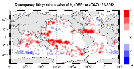
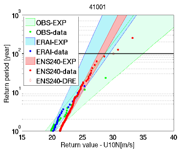
Because the ENS240 dataset is larger than the return period sought, it is possible to avoid extreme value analysis altogether and compute a non-parametric direct return estimate (DRE) from the tail of the empirical distribution function (see Appendix). Figs 1a and 2a show maps of the 100-yr return values of and , respectively. Estimates of and based on GP and the special case of the exponential distribution (EXP) closely resemble DRE in the extratropics (see Fig 3 and Fig 16), with estimates about 1.0 m s-1 below . Similarly, estimates are found to be within m of for most of the extratropics (Fig 3b). However, in the tropics the parametric estimates deviate significantly from DRE. The differences match closely areas visited by tropical cyclones, see eg Oouchi et al. (2006). EXP will yield significantly lower estimates compared with DRE while GP does the opposite. This is illustrated by Fig 4 where the confidence interval of fails to encompass the extremal values for a location in the subtropics. Tropical cyclones are underestimated in global numerical weather prediction models (Magnusson et al., 2014), thus the GP estimates come closer to the real return values in the affected areas, albeit still with large uncertainties and a large negative bias. It is interesting to note in passing that the highest wind speed found throughout the entire ensemble is close to 50 m s-1 while comes close to 25 m (see Fig 11).
3 Comparison With Traditional Return Estimates
Because ERA-I and the in situ observational time series are substantially shorter than the return period sought, we compare with ENS240 in terms of parametric return value estimates. ERA-I EXP estimates tend to exhibit a more stable behavior than GP estimates, and will be used in the following (see also Supplementary Material, Appendix B). In the extratropics the ENS240 estimates are 2-4 m s-1 higher than ERA-I (Fig 1b) while estimates are 1-3 m higher (Fig 2b). The situation is quite different in areas with tropical cyclones. Here we find much larger differences (more than 14 m s-1 for , see Fig 1b, and more than 6 m for , see Fig 2b). However, it is clear that the coarse resolution of the atmospheric model still renders tropical cyclones much too weak (Magnusson et al., 2014) compared to the maximum sustained wind speed observed under such weather systems (Elsner et al., 2008). This means that our wind speed estimates in the subtropics and the tropics should be considered lower bounds. It is worth remembering at this point, though, that the winds reported here must be considered averages over much longer periods (6 h) than the 10 minutes typically investigated in relation to tropical cyclones (Bidlot et al., 2002) (see Supplementary Material, Appendix B).
ENS240 is assumed to represent the equivalent of approximately 229 yrs. The size of the dataset reduces the confidence intervals to less than one third the width of ERA-I confidence intervals (34-yr dataset), see Figs 5 and 6. In general, ENS240 and compare reasonably well with POT estimates (see Appendix) of in situ observations (less than 10% difference except in areas with tropical cyclones, see Supplementary Material, Appendix B). These differences are within the expected uncertainties since return value estimates from observational time series of relatively short length (10-30 yrs) come with large confidence intervals. This is clearly seen for buoy 41001 east of Cape Hatteras (Fig 4), where estimates from ENS240 reveal yields 95% confidence intervals of 1 m s-1 while ERA-I has a width of about 4 m s-1 and the observations (1980-2012 with some gaps) in excess of 6 m s-1.
How do our return values compare with previous investigations? and exhibit the same geographical features as found by Caires and Sterl (2005) who calibrated the earlier ERA-40 reanalysis (Uppala et al., 2005) to in situ measurements of and . However, their fields are up to 6 m higher in the storm tracks in the North Atlantic and the North Pacific compared to what we find. No confidence intervals are provided, but a comparison of decadalwise return values shows approximately 10% spread in and in the extratropical storm tracks. Estimates of and based on aggregated altimeter measurements from satellite missions over the past 30 yrs (Vinoth and Young, 2011; Young et al., 2012) also yield much higher return values for wind speed in the extratropics. Wind speeds in excess of 52 m s-1 in the North Atlantic and the North Pacific are reported (Vinoth and Young, 2011; Young et al., 2012) using IDM. This is almost 50% higher than what we find and is likely to be an artefact of IDM, something which is also hinted at by the fact that the GP estimates (Vinoth and Young, 2011) fail to reproduce these extremes. For the results are much closer to our estimates. Since in the extratropics ENS240 compares well with in situ observations (both and ) and altimeter wind speed, we conclude that previous estimates (Caires and Sterl, 2005; Vinoth and Young, 2011; Young et al., 2012) are probably too high outside the subtropics and much too low in the tropics and subtropics (as are our estimates). Note that Caires and Sterl (2005) calibrated against 3-h averaged observations whereas Vinoth and Young (2011) and Young et al. (2012) assumed that the altimeter observations represented 3-h averages. This will lead to somewhat higher return values since we assume that the values are representative of 6-h interval. However, this can only explain a small fraction of the discrepancy (see Fig 10).
We note also that the investigation of 20-yr return values of from altimeter measurements by Izaguirre et al. (2011) yielded a positive shape parameter (unbounded extreme values) in areas with tropical cyclones, but a negative shape parameter (bounded extremes) in the extratropics. Their Fig 1 yields a map which is qualitatively very similar to Fig 3a.
4 Discussion
Implicit in the term “return value” lies the tacit assumption that the probability of non-exceedance is drawn from a long, stationary time series (Coles, 2001). In practice, observed and modeled time series vary in length from 30-100 yrs and are thus much shorter than the period over which stationarity is assumed, and with the exceptions of Compo et al. (2011), Wang et al. (2012) and Hersbach et al. (2013), the time series are also substantially shorter than the 100-yr return period. Decadal variations in storminess may affect these estimates (Caires and Sterl, 2005; Young et al., 2012) and climate projections of future wind and wave climate (Wang and Swail, 2006; Debernard and Røed, 2008; Hemer et al., 2013) suggest that nonstationary methods must be applied to assess future return values (see Kharin and Zwiers (2005), Izaguirre et al. (2010) and Izaguirre et al. (2011) for examples of nonstationary extreme value analysis). There is disagreement about the presence of trends in wave extremes in the extratropics (Wang and Swail, 2002; Caires and Sterl, 2005; Young et al., 2012), but there is some evidence (Young et al., 2012) that over the past three decades there has been a positive trend in extreme wind speed globally as well as in the intensity of tropical cyclones (Elsner et al., 2008). The trends in extreme wind speed (Young et al., 2012) are, however, based on 10-yr chunks of altimeter measurements and the uncertainties are very high. This is one of the strengths of using large aggregates of ensemble forecasts. These will by construct not exhibit long-term trends and low frequency oscillations since the initial conditions cover a period of 9 yrs. Stationarity is thus not an issue, suggesting that a similar approach could be used on short time slices (about 10 yrs) from ensembles covering several decades to avoid the complicating factors of using nonstationary methods. Candidate datasets that approach the size required would be reforecast ensembles (Hagedorn et al., 2012) and the recently completed 20th century model 10-member ensemble integrations (Hersbach et al., 2013). For climate projections multi-model ensembles (Hemer et al., 2013) could provide the amount of data necessary for extreme trend estimates.
Very large ensembles allow us to sidestep the choice of parametric distribution as we can compute direct 100-yr non-parametric return estimates. In principle, by looking at forecast ranges (briefly investigated by B13) instead of a fixed lead time it would be possible to perform a peaks-over-threshold analysis and increase the dataset by an order of magnitude. This would also remove any ambiguity concerning the representative interval of forecasts as the forecast range would determine the equivalent length of the dataset. Candidates for such an analysis would be for example the ECMWF monthly forecast system (Vitart et al., 2008), the extended forecast range of IFS from day 10 to day 15 and the seasonal forecast system (Stockdale et al., 2011; Molteni et al., 2011).
Using very large ensembles at advanced lead times is a novel method previously only explored for in the Northeast Atlantic (see B13). The method, like any method employing modeled fields, is sensitive to tail biases in the numerical model (Magnusson et al., 2014). These biases must be assessed for each new parameter, but in our case we find that they are moderate outside areas with tropical cyclones and significantly lower than those found for ERA-I. On the other hand, the unsystematic error associated with the parameter fitting to an extreme value distribution (Coles, 2001) is directly related to the size of the dataset and thus benefits immediately from an increase in size. The method is general and holds the promise of making much larger datasets available for a wide range of oceanographic, hydrological and meteorological parameters that are routinely forecast and archived.
Appendix A Methods Summary
The ENS240 forecasts were interpolated onto a regular grid. All +240-h forecasts (two per day, 00 and 12 UTC, 51 ensemble members in each) between 26 March 2003 and 25 March 2012 were used. ERA-I analyses (1979-2012) were interpolated onto the same grid. The current spectral truncation of ENS240 is T639 for the atmospheric model, corresponding to approximately 32 km, whereas the wave model ECWAM is run at approximately 55 km. Previous model cycles had coarser resolution, see Supplementary Material, Appendix B and B13. The 10-m neutral wind speed was extracted for both ENS240 and ERA-I. This is the field used to force the wave model and is thus consistent with the fields investigated. Grid points that are ice-covered in more than 20% of the forecasts were censored from the analysis of . No such censoring is required for .
We compared GP and EXP estimates and decided to use EXP for our comparison of ENS240 return values with ERA-I and in situ observations (see Supplementary Material, Appendix B). The threshold was set to the 1000th highest forecast, corresponding to . This choice (see Supplementary Material, Appendix B) was made after investigating the stability of EXP and GP estimates as a function of the threshold. Since ensemble forecasts are assumed uncorrelated, all values exceeding the threshold were used. For ERA-I and the in situ observations, the threshold was also set to and a POT technique applied where peaks must be separated by 48 h to ensure all entries are independent (Lopatoukhin et al., 2000; Coles, 2001). The distribution fitting was done with the maximum likelihood method and confidence intervals were estimated by bootstrapping. We found that 500 resamples were sufficient to yield a stable mean and a stable 95% confidence interval (see Supplementary Material, Appendix B). The threshold was set high enough to avoid summertime values. This means that in locations with strong seasonality in wind speed and direction our estimates should be interpreted as wintertime return values. We make no attempt to stratify the dataset by season or direction.
Under the assumption that the collection of +240-h forecast members are equivalent to a temporal period (each forecast representative of a 6-h interval, see Supplementary Material, Appendix B) we may convert our collection of ensemble forecasts into an equivalent time series. The two daily ensembles of +240-h forecasts from 50 perturbed ensemble members plus the unperturbed control member aggregated over 9 yrs can be considered to represent
| (1) |
We can therefore make non-parametric direct return estimates from the ensemble of the 100-yr return value, , without invoking a theoretical extreme value distribution (see Supplementary Material, Appendix B).
The assumption that the modeled wind and wave fields are representative of a 6-h interval is based on considerations of the horizontal model resolution (Bidlot et al., 2002). To test the sensitivity of the return value estimates to this assumption we have reduced the interval to 4 h, which is close to the averaging period used for the observations ( h). This reduction leads to an increase of at most 0.6 m for and 1.2 m s-1 for using the EXP distribution (Fig 10). This suggests that the method is reasonably insensitive to the choice of interval, but a little conservative.
All return estimates were computed marginally, i.e., per grid point. After that all fields were smoothed using a two-dimensional box-car filter after applying a smaller () MAX filter which selects the highest value from the nearest neighbours. This counters the tendency of the smoothing to lower the highest return values.
Appendix B Supplementary Material
The Supplementary Material is only available online in the article in Geophys Res Lett. Here, we include it as Appendix B. The figures thus form part of the manuscript and are numbered differently from the final version.
B.1 The ECMWF Integrated Forecast System (IFS) Ensemble
Since March 2003 IFS has been run twice daily to 10 days with 51 ensemble members (Buizza et al., 2007). As discussed by Breivik et al. (2013) (see their Fig 1), the resolution and the model physics of both the atmosphere and the wave components have undergone many revisions. The main changes in terms of resolution were upgrades to T399 from T255 in February 2006 and a further upgrade to T639 in February 2010. WAM followed this general increase in resolution with increases in spatial resolution from to in February 2010. The same subgrid scheme for unresolved bathymetry as was used for the ERA-I implementation was implemented in March 2004. For this investigation we have interpolated to the same regular longitude-latitude grid of as has been employed for the investigation of the ERA-I reanalysis.
B.2 ERA-Interim
ERA-Interim (ERA-I) is a global coupled atmosphere-wave ocean reanalysis starting in 1979 (Simmons et al., 2007; Uppala et al., 2008; Dee et al., 2011) based on Cycle 31r2 of IFS. The archive is extended in time regulary to be up to date. In this study the period covered is 1979-2012 (34 yrs). The archive has a resolution of for the wave model at the equator. An irregular latitude-longitude grid ensures relative constancy in grid resolution towards the poles. The atmospheric spectral truncation is T255 ( km), but atmospheric parameters are archived on a Gaussian grid of approximately . Both significant wave height and wind speed are interpolated to a regular longitude-latitude grid of resolution for this study. ERA-I employs a four-dimensional variational assimilation scheme. The ERA-I WAM model is coupled to the atmospheric model through exchange of the Charnock parameter (Janssen, 1989, 1991, 2004). The model incorporates shallow-water effects important in areas like the southern North Sea (Komen et al., 1994). ERA-I uses a subgrid scheme to represent the downstream impact of unresolved islands (Bidlot, 2012).
B.3 Model Tail Bias Assessed with In Situ and Altimeter Observations
To assess the tail behavior of the data sets we compare against 24 quality-controlled time series (Bidlot et al., 2002) of in situ measurements of 10-m wind speed, , and significant wave height, , in the northern hemisphere (Bidlot et al., 2002). To make the observations comparable with model output the observations are averaged over 5 h centered on the synoptic times. ENS240 wave fields are relatively coarse (approximately 50 km for T639 resolution) and should be considered representative of intervals of 4-6 h. We find good agreement at the 99.7% percentile () level for both and [see Fig 7, locations indicated in Fig 8]. ENVISAT RA2 altimeter observations of surface wind speed covering the period 2002-2012 were averaged into along-track “super-observations” (Janssen et al., 2007) of a resolution similar to the WAM model grid (Abdalla and Hersbach, 2004; Dragani et al., 2014). This procedure makes data and model values more comparable and serves the same purpose as the temporal averaging of in situ observations. Fig 8 shows that ERA-I is typically biased low by more than m s-1 in certain regions and about m s-1 globally. This is in contrast to ENS240 which is virtually unbiased when averaged globally and rarely deviates more than m s-1 locally.
As a further test of the tail behavior we have compared return values computed with the exponential distribution from in situ measurements (identical to how the ERA-I estimates were computed) to the ENS return estimates. As Fig 9 shows, the estimates match well, with less than 15% deviation in both wind speed and significant wave height except for in situ locations in the Gulf of Mexico exposed to tropical cyclones. As the time series for the in situ observations range from 10-30 yrs, there is large uncertainty in the estimates based on the observations. We would like to emphasize, as we do in the article, that tail (upper-percentile) biases may seriously affect the return value estimates. However, this is a problem always present when using model data for extreme value estimation, and is if anything less of a problem with the ENS240 dataset than with ERA-I, which tends to be biased low.
B.4 Estimating Return Values From Ensembles
Breivik et al (Breivik et al., 2013) laid down four criteria for using ensembles for extreme value estimation, restated slightly here as
-
1.
No significant correlation between ensemble members at advanced lead times
-
2.
The model climatology is comparable to the observed climatology distribution
-
3.
No spurious trend due to model updates
-
4.
Forecasts are representative of a time interval (e.g. 6 h)
Comparison with reforecast ensembles (Hagedorn et al., 2012) found (see Breivik et al. (2013)) no spurious trend in the mean and the variance of due to model upgrades.
As outlined by Breivik et al. (2013), converting ensemble forecasts with ensemble members each into the equivalent of a time period is necessary to go from probability of exceedance to return periods. We have assumed that each forecast represents a six-hour interval. The justification for this is firstly that matches the temporal resolution of ERA-I, hence making it easy to compare the results. Secondly, model fields are smoothly varying in time, making them representative of averages over typically 4-6 h at the resolution of ERA-I and ENS240. This allows us to treat the collection of ensemble forecasts as an equivalent time period . This averaging period coincides well with that used for the smoothing of the wave and wind observations (Bidlot et al., 2002), which is h. However, there is some arbitrariness in our choice of .
Parametric return estimates from ENS240 were found using the GP distribution for values exceeding a threshold such that , . The distribution can be written (Coles, 2001) as
| (2) |
Here is the shape parameter and is a scale parameter. In the limit as , , i.e., an exponential distribution (EXP) with parameter . We follow Coles (2001) and estimate return values with
| (3) |
| (4) |
| (5) |
Here represents the total number of data, is the total number of data per year, is total number of peaks above the threshold , is an estimate of the proportion of peaks above the threshold , is the -year return period, and and are the scale and shape parameter estimates obtained with the Maximum Likelihood Method (Coles, 2001). Assuming the reference period to be 6 hours
| (6) |
To investigate the impact of our choice of reference interval we recomput the return values using ,
| (7) |
In the extratropics the impact is modest (Fig 10) with at most an increase in of 0.6 m s-1 and 0.5 m for for EXP estimates. Areas prone to tropical cyclones east of Madagascar and in the South China Sea see an increase in of up to 1.2 m s-1. For the GP distribution (not shown) the discrepancy in will be larger in areas of , i.e. in areas visited by tropical cyclones, and smaller in areas with , i.e. in the extratropics, see Izaguirre et al. (2011).
It is also of interest to look at the absolute maxima obtained from the ensemble. Fig 11 shows that comes close to 50 m s-1 and reaches almost 25 m. The filtering effect of ocean waves is evident from the fact that the max field is spatially much smoother for than for .
B.5 Direct Return Estimates from Order Statistics
Consider a stationary time series of length where is the return period. By definition the highest entries are greater than the return value . Thus each of the periods contains on average one entry at least as large as . These highest entries are independent and spread randomly over the entire domain . Let represent the period of interest. Now is time measured in units of the return period. There is a probability that a randomly chosen interval of length does not contain a given entry . As becomes infinitely large the probability that the interval contains neither of the highest values is [Abramowitz and Stegun (1972), Eq (4.2.21)]
| (8) |
Here denotes the highest entry in . This result is independent of the underlying probability distribution as only the rank of the highest is of interest. It is now clear that some care has to be taken when interpreting the upper percentiles of even quite large datasets since according to Eq (8) the probability of exceeding the return value in any given return period is . Conversely, there is still a certain probability () that the 100-yr return value does not appear in our dataset of magnitude equivalent to 229 yrs ().
Our direct 100-yr estimate (DRE) taken from the order statistics of a dataset of this length is a linear interpolation between the second and third highest values [denoted and ] in the ordered sequence. The interpolation weight is found through the relation
| (9) |
where the fractions represent frequencies of occurrence of the second and third highest events as well as the 100-yr return event. Thus
| (10) |
B.6 Bootstrapping Confidence Intervals
Confidence intervals have been computed for ENS240 Generalized Pareto (GP) and exponential (EXP) distributions. It is interesting to compare the width of confidence intervals with those derived from ERA-I. With ERA-I we must perform a peaks-over-threshold (POT) selection of storm events, which is not applicable to the uncorrelated ENS240 data set. We have chosen in the main article to compare EXP return value estimates and used bootstraps of 500 resamples for the computation of the confidence intervals. The same relative differences are found for GP confidence intervals, although much wider in absolute terms (Fig 12b).
The bootstrap size must be large enough to provide a stable estimate of the return value but also of the confidence intervals. Efron (1987) demonstrated that in general bias-corrected accelerated (BCa) confidence intervals are preferable. We find that beyond a size of 500 the bootstrap yields very stable estimates of confidence intervals and average return values. Fig 13 demonstrates this clearly for the case with GP estimates (Panel a) and EXP estimates (Panel b) for a location in the Norwegian Sea.
B.7 Threshold Selection
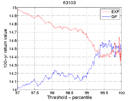
The threshold should ideally be chosen individually for each location (Aarnes et al., 2012), but this is clearly not feasible with a global dataset. We have chosen the level 99.7% after studying the behavior of both the GP and EXP estimates for a selection of locations. Fig 14 shows the behavior of the GP (blue) and EXP (red) estimates. The two estimates start to converge above 99% and are quite stable around 99.7%. This behavior with some variation is found throughout the extratropics. Selecting a threshold of 99.7% also means that the dataset contains only winter time storms in the extratropics and as such the estimates should clearly be seen as winter time return estimates. We make (as we stress in the main article) no attempt at stratifying our data by season or wind direction. To further investigate the impact of our choice of threshold we plot the global difference map between EXP estimates at and in Fig 15. As can be seen the estimates are not extremely sensitive to the choice of threshold except in areas with tropical cyclones. Given what we know from Fig 14 about the behavior of the return values for locations in the extratropics the threshold seems a reasonable choice.
B.8 Influence of the Shape Parameter
The shape parameter [see Eq (1)] is highly sensitive to the tail of the empirical distribution function. This can lead to spatially highly variable fields of return values. With data sets shorter than the return period, which is normally the case with observational records and model reanalyses, it may be difficult to find the shape parameter which best represents the conditions in a large geographical domain. Comparing the EXP distribution (, Fig 16) and the GP distribution (, see Fig 3) with the direct return estimates (DRE) reveals that for wind speed outside the tropics both EXP and GP agree well with DRE. However, in areas with tropical cyclones EXP tends to underestimate while GP yields return values substantially above DRE. GP may be a sensible choice for winds since our model results will tend to be biased low in the tropics as IFS is unable to capture the severity of tropical cyclones (Magnusson et al., 2014). For the picture is not quite so clear (contrast Fig 3b with Panel b of Fig 16), but the same general tendency for EXP to underestimate in areas with tropical cyclones lead us to conclude that GP is a better choice.
Acknowledgment
This work has been supported by the Research Council of Norway through the project “Wave Ensemble Prediction for Offshore Operations” (WEPO, grant no 200641) and through the European Union FP7 project MyWave (grant no 284455). SA was funded by the European Space Agency (contract 21519/08/I-OL, “Technical support for global validation of Envisat data products”). This study has also been part of a PhD program for OJA, partially funded by the Norwegian Centre for Offshore Wind Energy (NORCOWE). All datasets presented in this study are archived in ECMWF’s MARS database.
References
- Aarnes et al. (2012) Aarnes, O. J., Breivik, Ø., Reistad, M., 2012. Wave Extremes in the Northeast Atlantic. J Climate 25, 1529–1543.
- Abdalla and Hersbach (2004) Abdalla, S., Hersbach, H., 2004. The technical support for global validation of ERS Wind and Wave Products at ECMWF. ESA Contract Report 15988/02/I-LG, European Centre for Medium-Range Weather Forecasts.
- Abramowitz and Stegun (1972) Abramowitz, M., Stegun, I. A. (Eds.), 1972. Handbook of Mathematical Functions, with Formulas, Graphs, and Mathematical Tables. Dover, New York.
- Bidlot et al. (2002) Bidlot, J., Holmes, D., Wittmann, P., Lalbeharry, R., Chen, H., 2002. Intercomparison of the performance of operational ocean wave forecasting systems with buoy data. Wea Forecasting 17 (2), 287–310.
- Bidlot (2012) Bidlot, J.-R., 2012. Present status of wave forecasting at ECMWF. In: Workshop on Ocean Waves, 25-27 June 2012. Available online at http://www.ecmwf.int/publications/. p. 15.
- Breivik et al. (2013) Breivik, Ø., Aarnes, O. J., Bidlot, J.-R., Carrasco, A., Saetra, Ø., 2013. Wave Extremes in the North East Atlantic from Ensemble Forecasts. J Climate 26, 7525–7540, arXiv:1304.1354.
- Breivik et al. (2009) Breivik, Ø., Gusdal, Y., Furevik, B. R., Aarnes, O. J., Reistad, M., 2009. Nearshore wave forecasting and hindcasting by dynamical and statistical downscaling. J Marine Syst 78 (2), S235–S243, arXiv:1206.3055.
- Buizza et al. (2007) Buizza, R., Bidlot, J.-R., Wedi, N., Fuentes, M., Hamrud, M., Holt, G., Vitart, F., 2007. The new ECMWF VAREPS (Variable Resolution Ensemble Prediction System). Q J R Meteorol Soc 133 (624), 681–695.
- Caires and Sterl (2005) Caires, S., Sterl, A., 2005. 100-year return value estimates for ocean wind speed and significant wave height from the ERA-40 data. J Climate 18 (7), 1032–1048.
- Coles (2001) Coles, S., 2001. An introduction to statistical modeling of extreme values. Springer Verlag.
- Compo et al. (2011) Compo, G. P., Whitaker, J. S., Sardeshmukh, P. D., Matsui, N., Allan, R. J., Yin, X., Gleason, B. E., Vose, R. S., Rutledge, G., Bessemoulin, P., Brönnimann, S., Brunet, M., Crouthamel, R. I., Grant, A. N., Groisman, P. Y., Jones, P. D., Kruk, M. C., Kruger, A. C., Marshall, G. J., Maugeri, M., Mok, H. Y., Nordli, Ø., Ross, T. F., Trigo, R. M., Wang, X. L., Woodruff, S. D., Worley, S. J., 2011. The Twentieth Century Reanalysis Project. Q J R Meteorol Soc 137 (654), 1–28.
- Debernard and Røed (2008) Debernard, J., Røed, L. P., 2008. Future wind, wave and storm surge climate in the Northern Seas: a revisit. Tellus A 60, 427–438.
- Dee et al. (2011) Dee, D., Uppala, S., Simmons, A., Berrisford, P., Poli, P., Kobayashi, S., Andrae, U., Balmaseda, M., Balsamo, G., Bauer, P., P, B., Beljaars, A., van de Berg, L., Bidlot, J., Bormann, N., et al., 2011. The ERA-Interim reanalysis: Configuration and performance of the data assimilation system. Q J R Meteorol Soc 137 (656), 553–597.
- Dragani et al. (2014) Dragani, R., Abdalla, S., Engelen, R. J., Inness, A., Thépaut, J.-N., 2014. Ten years of ENVISAT observations at ECMWF: a review of activities and lessons learnt. Q J R Meteorol Soc, 23.
- Efron (1987) Efron, B., 1987. Better bootstrap confidence intervals. Journal of the American statistical Association 82 (397), 171–185.
- Elsner et al. (2008) Elsner, J. B., Kossin, J. P., Jagger, T. H., 2008. The increasing intensity of the strongest tropical cyclones. Nature 455 (7209), 92–95.
- Hagedorn et al. (2012) Hagedorn, R., Buizza, R., Hamill, T., Leutbecher, M., Palmer, T., 2012. Comparing TIGGE multimodel forecasts with reforecast-calibrated ECMWF ensemble forecasts. Q J R Meteorol Soc 138, 14.
- Hemer et al. (2013) Hemer, M. A., Fan, Y., Mori, N., Semedo, A., Wang, X. L., 2013. Projected changes in wave climate from a multi-model ensemble. Nature Climate Change 3 (5), 471–476.
- Hersbach et al. (2013) Hersbach, H., Peubey, C., Simmons, A., Poli, P., Dee, D., Berrisford, P., 2013. ERA-20CM: a twentieth century atmospheric model ensemble. ERA Report Series 16, European Centre for Medium-Range Weather Forecasts, http://www.ecmwf.int/publications.
- Izaguirre et al. (2011) Izaguirre, C., Méndez, F. J., Menéndez, M., Losada, I. J., 2011. Global extreme wave height variability based on satellite data. Geophys Res Lett 38 (10), 6.
- Izaguirre et al. (2010) Izaguirre, C., Mendez, F. J., Menendez, M., Luce o, A., Losada, I. J., 2010. Extreme wave climate variability in southern Europe using satellite data. J Geophys Res 115 (C4), 13.
- Janssen (1989) Janssen, P., 1989. Wave-induced stress and the drag of air flow over sea waves. J Phys Oceanogr 19 (6), 745–754, doi:10/fsz7vd.
- Janssen (1991) Janssen, P., 1991. Quasi-linear theory of wind-wave generation applied to wave forecasting. J Phys Oceanogr 21 (11), 1631–1642.
- Janssen (2004) Janssen, P., 2004. The interaction of ocean waves and wind. Cambridge University Press, Cambridge, UK.
- Janssen et al. (2007) Janssen, P. A., Abdalla, S., Hersbach, H., Bidlot, J.-R., 2007. Error estimation of buoy, satellite, and model wave height data. J Atmos Ocean Tech 24 (9), 1665–1677.
- Kalnay et al. (1996) Kalnay, E., Kanamitsu, M., Kistler, R., Collins, W., Deaven, D., Gandin, L., Iredell, M., Saha, S., White, G., Woollen, J., et al., 1996. The NCEP/NCAR 40-Year Reanalysis Project. Bull Am Meteor Soc 77, 437–472.
- Kharin and Zwiers (2005) Kharin, V., Zwiers, F., 2005. Estimating extremes in transient climate change simulations. J Climate 18 (8), 1156–1173.
- Komen et al. (1994) Komen, G. J., Cavaleri, L., Donelan, M., Hasselmann, K., Hasselmann, S., Janssen, P. A. E. M., 1994. Dynamics and Modelling of Ocean Waves. Cambridge University Press, Cambridge.
- Lopatoukhin et al. (2000) Lopatoukhin, L., Rozhkov, V., Ryabinin, V., Swail, V., Boukhanovsky, A., Degtyarev, A., 2000. Estimation of extreme wind wave heights. Tech. Rep. JCOMM Technical Report No 9, World Meteorological Organization.
- Magnusson et al. (2014) Magnusson, L., Bidlot, J.-R., Lang, S., Thorpe, A., Wedi, N., Yamaguchi, M., 2014. Evaluation of medium-range forecasts for hurricane Sandy. Mon Wea Rev, 48.
- Magnusson and Källén (2013) Magnusson, L., Källén, E., 2013. Factors Influencing Skill Improvements in the ECMWF Forecasting System. Mon Wea Rev, 3142–3153.
- Molteni et al. (2011) Molteni, F., Stockdale, T., Balmaseda, M. A., Balsamo, G., Buizza, R., Ferranti, L., Magnusson, L., Mogensen, K., Palmer, T. N., Vitart, F., 2011. The new ECMWF seasonal forecast system (System 4). ECMWF Technical Memorandum 656, European Centre for Medium-Range Weather Forecasts.
- Onogi et al. (2007) Onogi, K., Tsutsui, J., Koide, H., Sakamoto, M., Kobayashi, S., Hatsushika, H., Matsumoto, T., Yamazaki, N., Kamahori, H., Takahashi, K., et al., 2007. The JRA-25 reanalysis. J Meteorol Soc Jpn 85 (3), 369–432.
- Oouchi et al. (2006) Oouchi, K., Yoshimura, J., Yoshimura, H., Mizuta, R., Kusunoki, S., Noda, A., 2006. Tropical cyclone climatology in a global-warming climate as simulated in a 20 km-mesh global atmospheric model: Frequency and wind intensity analyses. Journal of the Meteorological Society of Japan 84 (2), 259–276.
- Reistad et al. (2011) Reistad, M., Breivik, Ø., Haakenstad, H., Aarnes, O. J., Furevik, B. R., Bidlot, J.-R., 2011. A high-resolution hindcast of wind and waves for the North Sea, the Norwegian Sea, and the Barents Sea. J Geophys Res 116, 18 pp, C05019.
- Rienecker et al. (2011) Rienecker, M. M., Suarez, M. J., Gelaro, R., Todling, R., Bacmeister, J., Liu, E., Bosilovich, M. G., Schubert, S. D., Takacs, L., Kim, G.-K., et al., 2011. MERRA: NASA’s Modern-Era Retrospective Analysis for Research and Applications. J Climate 24 (14), 3624–2648.
- Saha et al. (2013) Saha, S., Moorthi, S., Wu, X., Wang, J., Nadiga, S., Tripp, P., Behringer, D., Hou, Y.-T., Chuang, H.-y., Iredell, M., et al., 2013. The NCEP climate forecast system version 2. J Climate 27, 2185–2208.
- Simmons et al. (2007) Simmons, A., Uppala, S., Dee, D., Kobayashi, S., 2007. ERA-Interim: New ECMWF reanalysis products from 1989 onwards. ECMWF newsletter 110, 25–35.
- Stockdale et al. (2011) Stockdale, T., Anderson, D., Balmaseda, M., Doblas-Reyes, F., Ferranti, L., Mogensen, K., Palmer, T., Molteni, F., Vitart, F., 2011. ECMWF seasonal forecast system 3 and its prediction of sea surface temperature. Climate dynamics, 455–471, doi:10.1007/s00382–010–0947–3.
- Uppala et al. (2008) Uppala, S., Dee, D., Kobayashi, S., Berrisford, P., Simmons, A., 2008. Towards a climate data assimilation system: Status update of ERA-Interim. Ecmwf newsletter, European Centre for Medium-Range Weather Forecasts.
- Uppala et al. (2005) Uppala, S., Kållberg, P., Simmons, A., et al., 2005. The ERA-40 Re-analysis. Q J R Meteorol Soc 131, 2961–3012.
- Vinoth and Young (2011) Vinoth, J., Young, I., 2011. Global Estimates of Extreme Wind Speed and Wave Height. J Climate 24 (6), 1647–1665, doi:10.1175/2010JCLI3680.1.
- Vitart et al. (2008) Vitart, F., Balmaseda, R. B. M. A., Balsamo, G., Bidlot, J.-R., Bonet, A., Fuentes, M., Hofstadler, A., Molteni, F., Palmer, T. N., 2008. The new VarEPS-monthly forecasting system: A first step towards seamless prediction. Q J R Meteorol Soc 134 (636), 1789–1799.
- Wang et al. (2012) Wang, X., Feng, Y., Swail, V., 2012. North Atlantic wave height trends as reconstructed from the 20th Century Reanalysis. Geophys Res Lett 39, L18705, 6 pp.
- Wang and Swail (2001) Wang, X., Swail, V., 2001. Changes of extreme wave heights in Northern Hemisphere oceans and related atmospheric circulation regimes. J Climate 14 (10), 2204–2221.
- Wang and Swail (2002) Wang, X., Swail, V., 2002. Trends of Atlantic wave extremes as simulated in a 40-yr wave hindcast using kinematically reanalyzed wind fields. J Climate 15 (9), 1020–1035.
- Wang and Swail (2006) Wang, X., Swail, V., 2006. Climate change signal and uncertainty in projections of ocean wave heights. Climate Dynamics 26 (2), 109–126.
- Weisse and Günther (2007) Weisse, R., Günther, H., 2007. Wave climate and long-term changes for the Southern North Sea obtained from a high-resolution hindcast 1958–2002. Ocean Dynam 57 (3), 161–172.
- World Meteorological Organization (1998) World Meteorological Organization, 1998. Guide to wave analysis and forecasting. World Meteorological Organization, Geneva, Switzerland, 2nd Edition.
- Young et al. (2012) Young, I., Vinoth, J., Zieger, S., Babanin, A., 2012. Investigation of trends in extreme value wave height and wind speed. J Geophys Res 117 (C3), 13.
(a)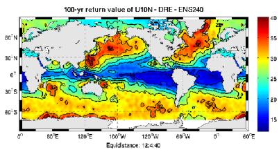
(b)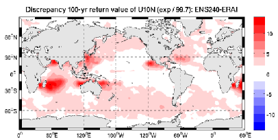
(a)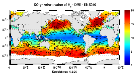
(b)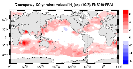
(a)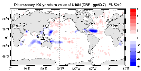
(b)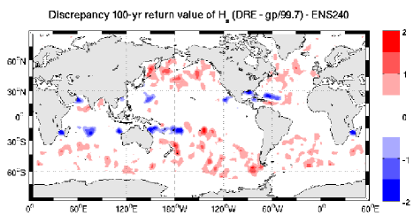
(a)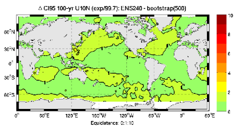
(b)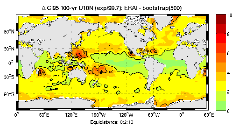
(a)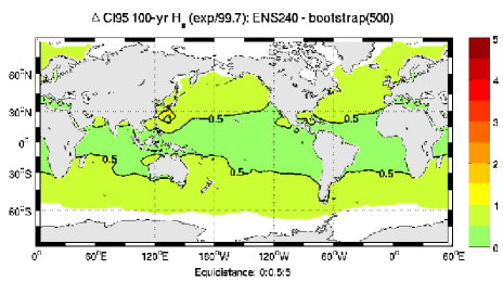
(b)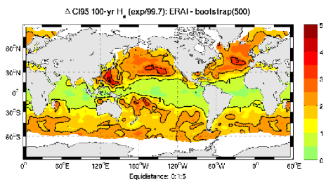
(a)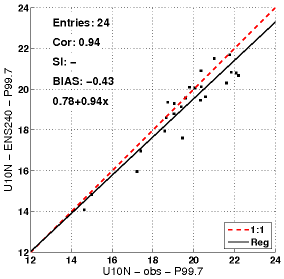
(b)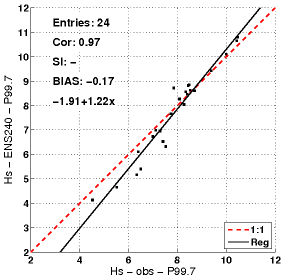
(a)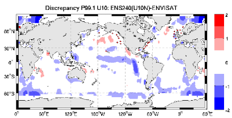
(b)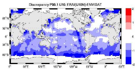
(a)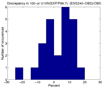
(b)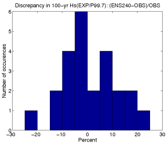
(a)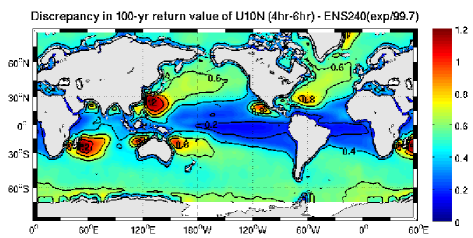
(b)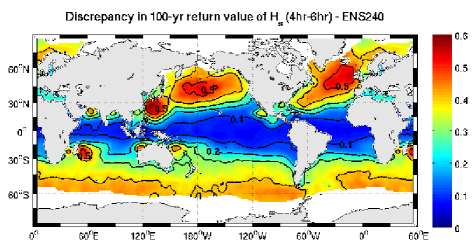
(a)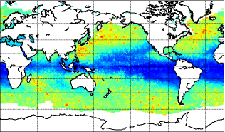
(b)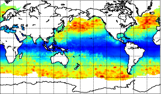
(a)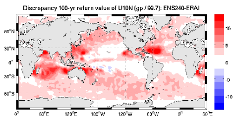
(b)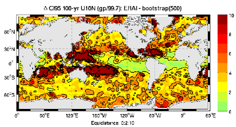
(a)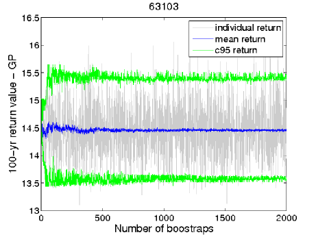
(b)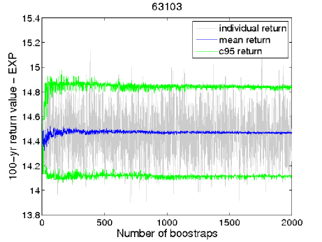
(a)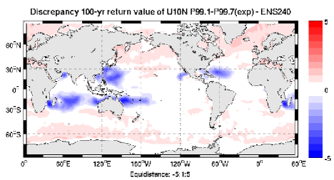
(b)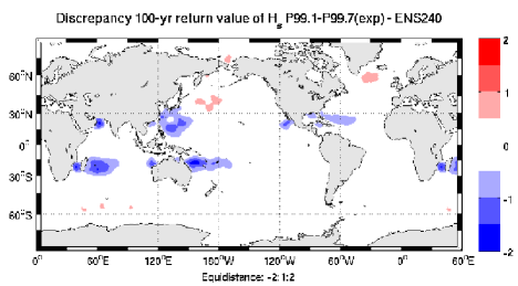
(a)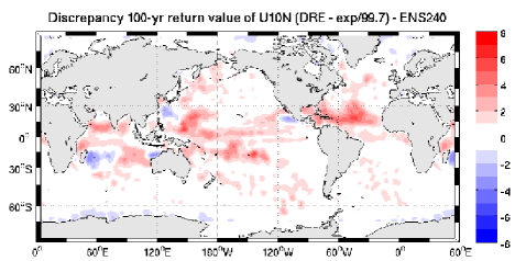
(b)