Equivalence between formulations in Cosmological Perturbation Theory: The primordial magnetic fields as an example.

Abstract

Nowdays, Cosmological Perturbation Theory is a standard and useful tool in theoretical cosmology. In this work, we compare the 1+3 covariant formalism in perturbation theory (Ellis et al.) to the gauge invariant approach (Bruni et al.), and we show the equivalence of these formalisms to fix the choice of the perturbed variables (gauge choice) in magnetogenesis. We analyze the evolution of primordial magnetic fields through perturbation theory and we discuss the similarities and differences between these two approaches. We get the Maxwell’s equations and show a cosmic dynamo like equation written in Poisson gauge, computing the evolution of primordial magnetic fields. Finally, prospects around these formalisms in the study of magnetogenesis are discussed.

La Teoría de Perturbaciones Cosmológicas es actualmente una herramienta estándar y útil en la cosmología teórica. En este trabajo se compara el formalismo covariante 1+3 de la teoría de perturbaciones (Ellis et al.) con la approximación invariante gauge (Bruni et al.), y mostramos la equivalencia de estos formalismos al fijar la escogencia de las variables perturbadas vía magnetogénesis. Se analiza la evolución de los campos magnéticos primordiales a través de la teoría de perturbaciones y se discuten las similitudes y diferencias entre estos dos enfoques. También se muestra las ecuaciones de Maxwell y la ecuación tipo dinamo cósmico escrita en el gauge Poisson el cual da cuenta de la evolución de los campos magnéticos primordiales. Por último, las perspectivas en torno a estos formalismos en el estudio de magnetogenesis son discutidos.

primordial magnetic fields Cosmological Perturbation Theory

0.1 Introduction

The origin of large scale magnetic fields is nowdays one of the major unsolved mysteries in cosmology. These fields are assumed to be increased and maintained by dynamo mechanism, but it needs a seed for the mechanism takes place (Widrow, 2002). Astrophysical mechanisms, as the Biermann battery have been used to explain how the magnetic field is mantained in objects as galaxies, stars and supernova remnants, but they are not likely correlated beyond galactic sizes making difficult to use astrophysical mechanisms to explain the origin of magnetic fields on cosmological scales (Kulsrun & Zweibel, 2008). In order to overcome this problem, the primordial origin should be found in other scenarios from which the astrophysical mechanism start. For example, magnetic fields could be generated during primordial phase transitions (such as QCD, the electroweak or GUT), parity-violating processes which generates magnetic helicity or during inflation (Grasso & Rubinstein, 2001). The advantage of these primordial processes is that they offer a wide range of coherence lengths many of which are strongly constrained by Nucleosynthesis, while the astrophysical mechanisms produce fields at the same order of the astrophysical size of the object (Kahniashvili et al., 2011). One way for describe the evolution of magnetic fields is through Cosmological Perturbation Theory. This theory is a powerful tool to understand the present properties of the large-scale structure of the Universe and their origin (for a review, see (Tsagas, 2002)). The main goal in this paper is to study the late evolution of magnetic fields which were generated in early stages of the universe. We use the cosmological perturbation theory following the Gauge Invariant formalism to find the perturbed Maxwell equations and also we obtain a dynamo like equation written in terms of gauge invariant variables. Futhermore, we discuss the importance that both curvature and the gravitational potential play in the evolution of these fields. The paper is organized as follows: in the next section § 0.2 we briefly give an introduction of cosmological perturbation theory and we address the gauge problem in this theory. In the section § 0.3 we consider the perturbed FLRW and we found the conservation equations at first order written in terms of gauge invariant quantities and the section § 0.5 a magnetic field in the FLRW background is introduced. Also a discussion between 1+3 covariant (Ellis et al., 1989) to the gauge invariant (Bruni et al., 1997) approaches is done in § 0.5. The final section § 0.6 is devoted to discuss the main results and the connection with future works.

0.2 The gauge problem in perturbation theory

Cosmological perturbation theory help us to find approximated solutions of the Einstein field equations through small desviations from an exact solution. The gauge invariant formalism is developed into two space-times, one is the real space-time $(\mathcal{M},g_{\alpha\beta})$ which describes the perturbed universe and the other one is the background space-time $(\mathcal{M}_{0},g_{\alpha\beta}^{(0)})$ which is an idealization and is taken as reference to generate the real space-time. A mapping between these space-times called gauge choice given by a function $\mathcal{X}:\>\mathcal{M}_{0}(p)\longrightarrow\mathcal{M}(\bar{p})$ for any point $p\in\mathcal{M}_{0}$ and $\bar{p}\in\mathcal{M}$, which generates a pull-back

$$\begin{array}[]{c}\mathcal{X}^{*}:\\ \\ \end{array}\;\begin{array}[]{c}\mathcal{M}\\ T^{*}(\overline{p})\end{array}\longrightarrow\begin{array}[]{c}\mathcal{M}_{0}\\ T^{*}(p)\end{array},$$ (1)

thus, points on the real and background space-time can be compared through of $\mathcal{X}$. General covariance states that there is no preferred coordinate system in nature and it introduce a gauge in perturbation theory. This gauge is an unphysical degree of freedom and we have to fix the gauge or to extract some invariant quantities to have physical results (Nakamura, 2009). Then, the perturbation for $\varGamma$ is defined as

$$\delta\varGamma(p)=\varGamma(\bar{p})-\varGamma^{(0)}(p).$$ (2)

We see that the perturbation $\delta\varGamma$ is completely dependent of the gauge choice because the mapping determines the representation on $\mathcal{M}_{0}$ of $\varGamma(\bar{p})$. However, one can also choice another correspondence $\mathcal{Y}$ between these space-times (see Figure 1) so that $\mathcal{Y}:\,\mathcal{M}_{0}(q)\rightarrow\mathcal{M}(\overline{p})$, ($p\neq q$). The freedom to choose different correspondences generate an arbitrariness in the value of $\delta\varGamma$ at any space-time point $p$, which is called gauge problem (Bardeen, 1980). Given a tensor field $\varGamma$ , the relations between first and second order perturbations of $\varGamma$ in two different gauges are

$$\delta^{(1)}_{\mathcal{Y}}\varGamma-\delta^{(1)}_{\mathcal{X}}\varGamma =\mathcal{L}_{\xi_{1}}\varGamma_{0},$$ (3)

$$\delta^{(2)}_{\mathcal{Y}}\varGamma-\delta^{(2)}_{\mathcal{X}}\varGamma =2\mathcal{L}_{\xi_{1}}\delta^{(1)}_{\mathcal{X}}\varGamma_{0}+\left(\mathcal{L}_{\xi_{1}}^{2}+\mathcal{L}_{\xi_{2}}\right)\varGamma_{0},$$ (4)

where the generators of the gauge transformation $\Phi$ are

$$\xi_{1}=Y-X\quad\text{and}\quad\xi_{2}=\left[X,Y\right].$$ (5)

This vector field can be split in their time and space part

$$\xi^{(r)}_{\mu}\rightarrow\left(\alpha^{(r)},\partial_{i}\beta^{(r)}+d_{i}^{(r)}\right),$$ (6)

here $\alpha^{(r)}$ and $\beta^{(r)}$ are arbitrary scalar functions, and $\partial^{i}d_{i}^{(r)}=0$. The function $\alpha_{(r)}$ determines the choice of constant time hypersurfaces, while $\partial_{i}\beta^{(r)}$ and $d_{i}^{(r)}$ fix the spatial coordinates within these hypersurfaces. The choice of coordinates is arbitrary and the definitions of perturbations are thus gauge dependent.

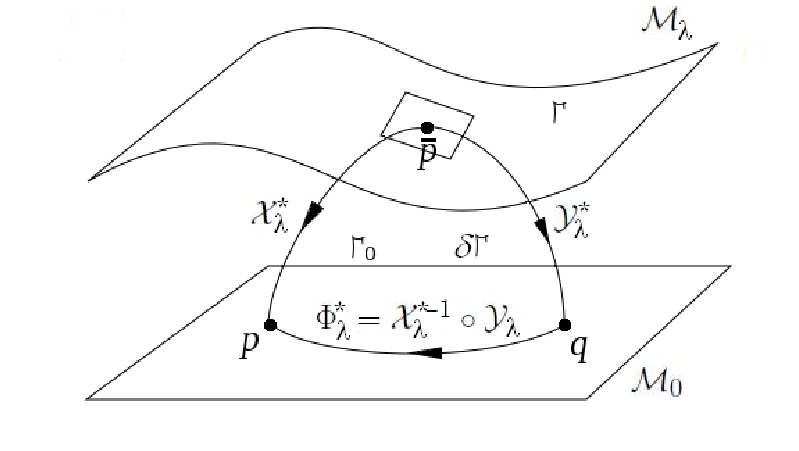
Figure 1: Gauge Transformation.

The gauge transformation given by the equations (3) and (4) are quite general. To first order $\varGamma$ is gauge invariant if $\mathcal{L}_{\xi_{1}}\varGamma_{0}=0$, while to second order one must have another conditions $\mathcal{L}_{\xi_{1}}\delta^{(1)}_{\mathcal{X}}\varGamma_{0}=\mathcal{L}_{\xi_{1}}^{2}\varGamma_{0}=0$ and $\mathcal{L}_{\xi_{2}}\varGamma_{0}=0$, and so on at high orders (Stewart & Walker, 1974). We will apply the formalism described above to the Robertson-Walker metric, where $k$ does mention the expansion order.

0.3 Gauge invariant variables at first order

We consider the perturbations about a FLRW background, so the metric tensor is given by :

$$g_{00} =-a^{2}(\tau)\left(1+2\sum_{k=1}^{\infty}\frac{1}{k!}\psi^{(k)}\right),$$ (7)

$$g_{0i} =a^{2}(\tau)\sum_{k=1}^{\infty}\frac{1}{k!}\omega_{i}^{(k)},$$ (8)

$$g_{ij} =a^{2}(\tau)\left[\left(1-2\sum_{k=1}^{\infty}\frac{1}{k!}\phi^{(k)}\right)\delta_{ij}\right.\left.+\sum_{k=1}^{\infty}\frac{\chi_{ij}^{(k)}}{k!}\right].$$ (9)

The perturbations are splitting into scalar, transverse vector part, and transverse trace-free tensor

$$\omega_{i}^{(k)}=\partial_{i}\omega^{(k)\|}+\omega_{i}^{(k)\bot},$$ (10)

with $\partial^{i}\omega_{i}^{(k)\bot}=0$. Similarly we can split $\chi_{ij}^{(k)}$ as

$$\chi_{ij}^{(k)}=D_{ij}\chi^{(k)\|}+\partial_{i}\chi_{j}^{(k)\bot}+\partial_{j}\chi_{i}^{(k)\bot}+\chi_{ij}^{(k)\top},$$ (11)

for any tensor quantity. Following, one can find the scalar gauge invariant variables at first order given by

$$\Psi^{(1)} \equiv \psi^{(1)}+\frac{1}{a}\left(\mathcal{S}_{(1)}^{||}a\right)^{\prime},$$ (12)

$$\Phi^{(1)} \equiv \phi^{(1)}+\frac{1}{6}\nabla^{2}\chi^{(1)}-H\mathcal{S}_{(1)}^{||},$$ (13)

$$\Delta^{(1)} \equiv \mu_{(1)}+\left(\mu_{(0)}\right)^{\prime}\mathcal{S}_{(1)}^{||},$$ (14)

$$\Delta^{(1)}_{P} \equiv P_{(1)}+\left(P_{(0)}\right)^{\prime}\mathcal{S}_{(1)}^{||},$$ (15)

with $\mathcal{S}_{(1)}^{||}\equiv\left(\omega^{||(1)}-\frac{\left(\chi^{||(1)}\right)^{\prime}}{2}\right)$ the scalar contribution of the shear. The vector modes are

$${\upsilon}_{(1)}^{i} \equiv v_{(1)}^{i}+\left(\chi_{\bot(1)}^{i}\right)^{\prime},$$ (16)

$$\vartheta_{i}^{(1)} \equiv \omega_{i}^{(1)}-\left(\chi_{i}^{\bot(1)}\right)^{\prime},$$ (17)

$$\mathcal{V}_{(1)}^{i} \equiv \omega_{(1)}^{i}+v_{(1)}^{i}.$$ (18)

$$\mu=\mu_{0}+\sum_{r=1}^{\infty}\frac{1}{r!}\delta^{r}\mu,\,u^{\alpha}=\frac{1}{a}\left(\delta_{0}^{\alpha}+\sum_{r=1}^{\infty}\frac{1}{r!}v_{(r)}^{\alpha}\right)$$ (19)

with $\mathcal{S}_{(1)}^{||}\equiv\left(\omega^{||(1)}-\frac{\left(\chi^{||(1)}\right)^{\prime}}{2}\right)$ the scalar contribution of the shear (associated with $\alpha^{(1)}$). Using the Einstein’s equation at first order, it is expressed the evolution of geometrical variables $\phi$ and $\psi$, and the conservation’s equations entails the evolution of energy density $\Delta^{(1)}$

$$\left(\Delta^{(1)}\right)^{\prime}+3H\left(\Delta_{P}^{(1)}+\Delta^{(1)}\right)$$ (20)

$$- 3\left(\Phi^{(1)}\right)^{\prime}\left(P_{(0)}+\mu_{(0)}\right)+\left(P_{(0)}+\mu_{(0)}\right)\nabla^{2}\upsilon^{(1)}$$

$$- 3H\left(P_{(0)}+\mu_{(0)}\right)^{\prime}\mathcal{S}_{(1)}^{||}-\left(\left(\mu_{(0)}\right)^{\prime}\mathcal{S}_{(1)}^{||}\right)^{\prime}$$

$$+ \left(P_{(0)}+\mu_{(0)}\right)\left(-\frac{1}{2}\nabla^{2}\chi^{(1)}+3H\mathcal{S}_{(1)}^{||}\right)^{\prime}$$

$$- \left(P_{(0)}+\mu_{(0)}\right)\nabla^{2}\left(\frac{1}{2}\chi^{||(1)}\right)^{\prime}=0,$$

and peculiar velocity $\mathcal{V}_{(1)}$ given by

$$\left(\mathcal{V}_{i}^{(1)}\right)^{\prime}+\frac{\left(\mu_{(0)}+P_{(0)}\right)^{\prime}}{\left(\mu_{(0)}+P_{(0)}\right)}\mathcal{V}_{i}^{(1)}-4H\mathcal{V}_{i}^{(1)}+\partial_{i}\Psi^{(1)}$$ (21)

$$- \frac{{}_{\partial_{i}\left(\Delta_{P}^{(1)}-\left(P_{(0)}\right)^{\prime}\mathcal{S}_{(1)}^{||}\right)+\partial_{l}\Pi_{(fl)i}^{(1)l}}}{\left(\mu_{(0)}+P_{(0)}\right)}=\frac{\partial_{i}\left(\mathcal{S}_{(1)}^{||}a\right)^{\prime}}{a}.$$

0.4 Specifying to Poisson gauge

It is possible to fix the four degrees of freedom by imposing gauge conditions. If we impose the gauge restrictions given in (Bertschinger, 1995) we can removing the degrees of freedom, we fix the gauge conditions as

$$\partial^{i}\omega_{i}^{(r)}=\partial^{i}\chi_{ij}^{(r)}=0,$$ (22)

this lead to some functions are dropped

$$\omega^{\parallel(r)}=\chi^{(r)\bot}_{i}=\chi^{(r)\parallel}=0,$$ (23)

with the functions defined in equations (10) and (11). Using the last constraints together with equations (5.18)-(5.21) in (Bruni et al., 1997) and following the procedure made in (Malik & Wands, 2009), the vector which determines the gauge transformation at first order $\xi_{i}^{(1)}=\left(\alpha^{(1)},\partial_{i}\beta^{(1)}+d^{(1)}_{i}\right)$ is given by,

$$\alpha^{(1)}\rightarrow\omega_{(1)}^{\parallel}+\beta^{\prime}_{(1)},\quad\beta^{(1)}\rightarrow-\frac{\chi^{\parallel(1)}}{2},\quad d_{i}^{(1)}\rightarrow-\chi^{\bot(1)}_{i}.$$ (24)

0.5 Weakly magnetized FLRW-background

We allow the presence of a weak magnetic field into our FLRW space-time with the property $B_{(0)}^{2}\ll\mu_{(0)}$ and must be sufficiently random to satisface $\left\langle B_{i}\right\rangle=0$ and $\left\langle B_{(0)}^{2}\right\rangle\neq 0$ to ensure that symmetries and the evolution of the background remain unaffected (we assume that at zero order the magnetic field has been generated by some random process which is statistically homogeneous so that $B_{(0)}^{2}$ just time depending and $\left\langle..\right\rangle$ denotes the expectation value) (Barrow et al., 2007). We work under MHD approximation, thus, in large scales the plasma is globally neutral, charge density is neglected and the electric field with the current should be zero, thus the only zero order magnetic variable is $B_{(0)}^{2}$. At first order it is obtained a gauge invariant term which describes the magnetic energy density

$$\Delta^{(1)}_{mag}\equiv\ B_{(1)}^{2}+\left(B_{(0)}^{2}\right)^{\prime}\alpha^{(1)}.$$ (25)

Another gauge invariant variables are the 3-current $J$, the charge density $\varrho$ and the electric and magnetic fields, because they vanish in the background.
At first order, the electric field and the current become nonzero and assuming the ohmic current is not neglected, we find the Ohm’s law

$$J_{i}^{(1)}=\sigma\left[E_{i}^{(1)}+\left(\mathcal{V}^{(1)}\times B^{(0)}\right)_{i}\right].$$ (26)

The perturbed equations for the metric and electromagnetic fields are given by

$$\partial_{i}E_{(1)}^{i}=a\varrho_{(1)},\quad\epsilon^{ilk}\partial_{l}B^{(1)}_{k}=\left(a^{2}E_{(1)}^{i}\right)^{\prime}+a^{3}J_{(1)}^{i},$$

$$\partial^{i}B_{i}^{(1)}=0,\quad\left(a^{2}B_{k}^{(1)}\right)^{\prime}+a^{2}\epsilon_{\>k}^{ij}\partial_{i}E_{j}^{(1)}=0.$$ (27)

Now using equation (27) together with the Ohm’s law, we get a cosmic dynamo like equation which describes the evolution of density magnetic field at first order in the Poisson gauge

$$\frac{d\Delta_{(mag)}^{(2)}}{dt}+4H\Delta_{(mag)}^{(2)}+2\eta\mathcal{\epsilon}^{(2)}$$

$$+\frac{2}{3}\Delta_{(mag)}^{(1)}\partial_{l}\mathcal{V}_{(1)}^{l}=-2\Pi^{(1)}_{ij(em)}\sigma^{ij}_{(1)},$$ (28)

with $\mathcal{\epsilon}^{(2)}$ given by

$$\mathcal{\epsilon}^{(2)}=-B^{(1)}\cdot\nabla^{2}B^{(1)}$$

$$-B^{(1)}_{k}\left(\nabla\times\left(\frac{dE_{(1)}}{dt}+2HE_{(1)}\right)\right)^{k}$$

$$-\frac{\Delta_{(mag)}^{(1)}}{2}\nabla^{2}\left(\Psi^{(1)}-3\Phi^{(1)}\right)$$

$$+B^{k}_{(1)}\left(B^{(0)}\cdot\nabla\right)\partial_{k}\left(\Psi^{(1)}-3\Phi^{(1)}\right),$$ (29)

where we use the Lagrangian coordinates which are comoving with the local Hubble flow and magnetic field lines are frozen into the fluid ($\dfrac{d}{dt}=\dfrac{\partial}{\partial t}+\mathcal{V}_{(1)}^{i}\partial_{i}$), $\sigma$ and $\Pi$ are the shear and stress Maxwell tensor respectively. Thus, the perturbations in the space-time play an important role in the evolution of primordial magnetic fields (Hortúa et al., 2011). In the case of a homogeneous collapse, $B\sim\mathcal{V}^{-\frac{2}{3}}$ there is an amplification of the magnetic field in places where gravitational collapse take place. In equation (28), the energy density magnetic field at second order transforms as

$$\Delta_{(mag)}^{(2)}=B^{2}_{(2)}+\alpha_{(1)}\left(B^{2\prime\prime}_{(0)}\alpha_{(1)}+B^{2\prime}_{(0)}\alpha_{(1)}^{\prime}+2B^{2\prime}_{(1)}\right)$$

$$+\xi^{i}_{(1)}\left(B^{2\prime}_{(0)}\partial_{i}\alpha^{(1)}+2\partial_{i}B^{2}_{(1)}\right)+B^{2\prime}_{(0)}\alpha_{(2)}.$$ (30)

Finally, we relate quantities in the 1+3 covariant formalism and in the invariant approach showed above. In the covariant formalism quantities are projected down onto spatial $h_{\alpha\beta}$, relative to the 4-velocity of the fluid. With this choice, we expect that covariant formalism could be equivalent to comoving gauge (Tsagas et al., 2000). The comoving magnetic density gradient is defined as

$${\cal B}_{\mu}\equiv\frac{a}{B^{2}}h^{\lambda}_{\mu}\nabla_{\lambda}B^{2},\quad\text{with}\quad h_{\mu\nu}\equiv g_{\mu\nu}+u_{\mu}u_{\nu}\,.$$ (31)

Now, following (Malik et al., 2012) we substitute the 4-velocity at first order found in gauge invariant approach $u_{\mu}=a\left(-(1+\psi),\ \partial_{i}(v^{\parallel}+\omega^{\parallel})\right)\,$, obtaining the following relation

$$h^{\lambda}_{\mu}\nabla_{\lambda}B^{2}=\partial_{i}\left(B^{2}_{(1)}+B^{2\prime}_{(0)}\left(v^{\parallel}+\omega^{\parallel}\right)\right)\,.$$ (32)

If the comoving gauge is used (which introduces a family of world lines orthogonal to the 3-D spatial sections) given by $\alpha\rightarrow v^{\parallel}+\omega^{\parallel}$ in equation (25), is derived a similar to expression as it was found in 1+3 covariant formalism in equation (32), implying an equivalence in both formalisms at linear order. Now, if we study this equivalence at second order, we must impose $u_{i}^{(2)}=0$ to provide a covariant description (due to we must ensure 4-velocity orthogonal to 3D spatial sections). In this case the 4-velocity at second order is

$$\frac{u_{i}^{(2)}}{a}=\left[\frac{(v_{i}^{(2)}+\omega_{i}^{(2)})}{2}-2v_{i}^{(1)}\phi^{(1)}-\omega^{(1)}_{i}\psi_{(1)}+v^{j}_{(1)}\chi_{ij}^{(1)}\right]\,$$ (33)

in (Hortúa, 2012) is shown vector field that determines the gauge comoving at second order. In this case one must take into account that 4-velocity must be zero and choose appropriately the 3D spatial section through of $\beta^{(2)}$ and $d_{i}^{(2)}$.

0.6 discussion

A problem in modern cosmology is to explain the origin of cosmic magnetic fields. The origin of these fields is still in debate but they must affect the formation of large scale structure and the anisotropies in the cosmic microwave background radiation (CMB) (Giovannini et al., 2008). We observe that essentially, the functional form are the same in the two approaches, the coupling between geometrical perturbations and fields variables appear as sources in the magnetic field evolution giving a new possibility to explain the amplification of primordial cosmic magnetic fields. Thus the perturbations in the space-time play an important role in the evolution of primordial magnetic fields. The equation (28) is dependent on geometrical quantities (perturbation in the gravitational potential, curvature, velocity …). These quantities evolve according to the Einstein field equations (the Einstein field equation to second order are given in (Nakamura, 2007)). In this way, the equation equation (28) tell us how the magnetic field evolves according to scale of the perturbation. In sub-horizon scale, the contrast density and the geometrical quantities grow. Hence, is expected that naturally the dynamo term should amplify the magnetic field.

References

- Widrow (2002) Widrow, L. M. 2006, Reviews of Modern Physics, 74, 775
- Kulsrun & Zweibel (2008) Kulsrud, R. M., & Zweibel, E. G. 2008, Reports on Progress in Physics , 71, 4
- Grasso & Rubinstein (2001) Grasso, D., & Rubinstein, H. R. 2001, Phys. Rep., 348, 163
- Kahniashvili et al. (2011) Kahniashvili, T., Tevzadze, A. G., & Ratra, B. 2011, ApJ, 726, 78
- Tsagas (2002) Tsagas, C. G. 2002, Lecture Notes in Physics, Berlin Springer Verlag, 592, 223
- Ellis et al. (1989) Ellis, G. F. R., & Bruni, M. 1989, Phys. Rev. D, 40, 1804
- Bruni et al. (1997) Bruni, M., Matarrese, S., Mollerach, S., & Sonego, S. 1997,Classical and Quantum Gravity, 14, 2585
- Nakamura (2009) Nakamura, K. 2009, Phys. Rev. D, 80, 124021
- Bardeen (1980) Bardeen, J. M. 1980, Phys. Rev. D, 22, 1882
- Stewart & Walker (1974) Stewart J. M., & Walker M. 1974, Proc. R. Soc. London, A471, 49
- Bertschinger (1995) Bertschinger, E. 1995, NASA STI/Recon Technical Report N, 96, 22249
- Malik & Wands (2009) Malik, K. A., & Wands, D. 2009, Phys. Rep., 475, 1
- Tsagas et al. (2000) Tsagas, C., & Maartens, R. 2000, Phys. Rev. D, 61, 083519
- Hortúa et al. (2011) Hortúa, H. J., Castañeda, L., & Tejeiro, J. M. 2011, in press (arXiv:1104.0701v3)
- Hortúa (2012) Hortúa, H. J. 2012, Tesís de Maestría (Generation of primordial magnetic fields) http://www.bdigital.unal.edu.co/7747/)
- Barrow et al. (2007) Barrow, J. D., Maartens, R., & Tsagas, C. G. 1954, Phys. Rep., 449, 131
- Malik et al. (2012) Malik, K. A., & Matravers, D. R. 2012, in press (arXiv:1206.1478v3)
- Nakamura (2007) Nakamura, K. 2007, Progress of Theoretical Physics, 117, 17
- Giovannini et al. (2008) Giovannini, M., & Kunze, K. E. 2008, Phys. Rev. D, 77, 6