Tractable Model for Rate in Self-Backhauled Millimeter Wave Cellular Networks

Abstract

Millimeter wave (mmWave) cellular systems will require high gain directional antennas and dense base station (BS) deployments to overcome high near field path loss and poor diffraction. As a desirable side effect, high gain antennas offer interference isolation, providing an opportunity to incorporate self-backhauling–BSs backhauling among themselves in a mesh architecture without significant loss in throughput–to enable the requisite large BS densities. The use of directional antennas and resource sharing between access and backhaul links leads to coverage and rate trends that differ significantly from conventional ultra high frequency (UHF) cellular systems. In this paper, we propose a general and tractable mmWave cellular model capturing these key trends and characterize the associated rate distribution. The developed model and analysis is validated using actual building locations from dense urban settings and empirically-derived path loss models. The analysis shows that in sharp contrast to the interference-limited nature of UHF cellular networks, the spectral efficiency of mmWave networks (besides total rate) also increases with BS density particularly at the cell edge. Increasing the system bandwidth, although boosting median and peak rates, does not significantly influence the cell edge rate. With self-backhauling, different combinations of the wired backhaul fraction (i.e. the fraction of BSs with a wired connection) and BS density are shown to guarantee the same median rate (QoS).

I Introduction

The scarcity of “beachfront” UHF ($300$ MHz- $3$ GHz) spectrum and surging wireless traffic demands has made going higher in frequency for terrestrial communications inevitable. The capacity boost provided by increased Long Term Evolution (LTE) deployments and aggressive small cell, particularly Wi-Fi, offloading has, so far, been able to cater to the increasing traffic demands, but to meet the projected [2] traffic needs of $2020$ (and beyond) availability of large amounts of new spectrum would be indispensable. The only place where a significant amount of unused or lightly used spectrum is available is in the millimeter wave (mmWave) bands ($20-100$ GHz). With many GHz of spectrum to offer, mmWave bands are becoming increasingly attractive as one of the front runners for the next generation (a.k.a. “$5$G”) wireless cellular networks [3, 4, 5].

I-A Background and recent work

Feasibility of mmWave cellular. Although mmWave based indoor and personal area networks have already received considerable traction [6, 7], such frequencies have long been deemed unattractive for cellular communications primarily due to the large near-field loss and poor penetration (blocking) through concrete, water, foliage, and other common material. Recent research efforts [8, 4, 9, 10, 11, 12, 13, 14] have, however, seriously challenged this widespread perception. In principle, the smaller wavelengths associated with mmWave allow placing many more miniaturized antennas in the same physical area, thus compensating for the near-field path loss [8, 9]. Communication ranges of 150-200m have been shown to be feasible in dense urban scenarios with the use of such high gain directional antennas [4, 10, 9]. Although mmWave signals do indeed penetrate and diffract poorly through urban clutter, dense urban environments offer rich multipath (at least for outdoor) with strong reflections; making non-line-of-sight (NLOS) communication feasible with familiar path loss exponents in the range of $3$-$4$ [4, 9]. Dense and directional mmWave networks have been shown to exhibit a similar spectral efficiency to $4$G (LTE) networks (of the same density) [11, 12], and hence can achieve an order of magnitude gain in throughput due to the increased bandwidth.

Coverage trends in mmWave cellular. With high gain directional antennas and newfound sensitivity to blocking, mmWave coverage trends will be quite different from previous cellular networks. Investigations via detailed system level simulations [11, 12, 15, 13, 14, 16] have shown large bandwidth mmWave networks in urban settings tend to be noise limited–i.e. thermal noise dominates interference–in contrast to $4$G cellular networks, which are usually strongly interference limited. As a result, mmWave outages are mostly due to a low signal-to-noise-ratio ($\mathtt{SNR}$) instead of low signal-to-interference-ratio ($\mathtt{SIR}$). This insight was also highlighted in an earlier work [17] for directional mmWave ad hoc networks. Because cell edge users experience low $\mathtt{SNR}$ and are power limited, increased bandwidth leads to little or no gain in their rates as compared to the median or peak rates [12]. Note that rates were compared with a $4$G network in [12], however, in this paper we also investigate the effect of bandwidth on rate in mmWave regime.

Density and backhaul. As highlighted in [13, 11, 12, 8, 15, 14], dense BS deployments are essential for mmWave networks to achieve acceptable coverage and rate. This poses a particular challenge for the backhaul network, especially given the huge rates stemming from mmWave bandwidths on the order of GHz. However, the interference isolation provided by narrow directional beams provides a unique opportunity for scalable backhaul architectures [8, 18, 19]. Specifically, self-backhauling is a natural and scalable solution [18, 19, 20], where BSs with wired backhaul provide for the backhaul of BSs without it using a mmWave link. This architecture is quite different from the mmWave based point-to-point backhaul [21] or the relaying architecture [22] already in use, as (a) the BS with wired backhaul serves multiple BSs, and (b) access and backhaul links share the total pool of available resources at each BS . This results in a multihop network, but one in which the hops need not interfere, which is what largely doomed previous attempts at mesh networking. However, both the load on the backhaul and access link impact the eventual user rate, and a general and tractable model that integrates the backhauling architecture into the analysis of a mmWave cellular network seems important to develop. The main objective of this work is to address this. As we show, the very notion of a coverage/association cell is strongly questionable due to the sensitivity of mmWave to blocking in dense urban scenarios. Characterizing the load and rate in such networks, therefore, is non-trivial due to the formation of irregular and “chaotic” association cells (see Fig. 3).

Relevant models. Recent work in developing models for the analysis of mmWave cellular networks (ignoring backhaul) includes [23, 24, 25], where the downlink $\mathtt{SINR}$ distribution is characterized assuming BSs to be spatially distributed according to a Poisson point process (PPP). No blockages were assumed in [23], while [24] proposed a framework to derive $\mathtt{SINR}$ distribution with an isotropic blockage model, and derived the expressions for a line of sight (LOS) ball based blockage model in which all nearby BSs were assumed LOS and all BSs beyond a certain distance from the user were ignored. This LOS ball blockage model can be interpreted as a step function approximation of the exponential blockage model proposed in [26] and used in [25]. The randomness in the distance-based path loss (shown to be quite significant in empirical studies [14]), was however ignored in prior analytical works. Coverage was shown [24] to exhibit a non-monotonic trend with BS density. In this work, however, we show that if the finite user population is taken into account (ignored in [24]), $\mathtt{SINR}$ coverage may increase monotonically with density. Although characterizing $\mathtt{SINR}$ is important, rate is the key metric, and can follow quite different trends [27, 28] than $\mathtt{SINR}$ because the user load is essentially a pre-log factor whereas $\mathtt{SINR}$ is inside the log in the Shannon capacity formula.

I-B Contributions

The major contributions of this paper can be categorized broadly as follows:
Tractable mmWave cellular model. A tractable and general model is proposed in Sec. II for characterizing coverage and rate distribution in self-backhauled mmWave cellular networks. The proposed blockage model allows for an adaptive fraction of area around each user to be LOS. Assuming the BSs are distributed according to a PPP, the analysis, developed in Sec. III, accounts for different path losses (both mean and variance) of LOS/NLOS links for both access and backhaul–consistent with empirical studies [4, 14]. We identify and characterize two types of association cells in self-backhauled networks: (a) user association areaof a BS which impacts the load on the access link, and (b) BS association areaof a BS with wired backhaul required for quantifying the load on the backhaul link. The rate distribution across the entire network, accounting for the random backhaul and access link capacity, is then characterized in Sec III. Further, the analysis is extended to derive the rate distribution with offloading to and from a co-existing UHF macrocellular network.
Validation of model and analysis. In Sec. III-E, the analytical rate distribution derived from the proposed model is compared with that obtained from simulations employing actual building locations in dense urban regions of New York and Chicago [16], and empirically measured path loss models [14]. The demonstrated close match between the analysis and simulation validates the proposed blockage model and our analytical approximation of the irregular association areas and load.
Performance insights. Using the developed framework, it is demonstrated in Sec. IV that:

• MmWave networks in dense urban scenarios employing high gain narrow beam antennas tend to be noise-limited for “moderate” BS densities. Consequently, densification of the network improves the $\mathtt{SINR}$ coverage, especially for uplink. Incorporating the impact of finite user density, $\mathtt{SINR}$ coverage can possibly increase with density even in the very large density regime.

• Cell edge users experience poor $\mathtt{SNR}$ and hence are particularly power limited. Increasing the air interface bandwidth, as a result, does not significantly improve the cell edge rate, in contrast to the cell median or peak rates. Improving the density, however, improves the cell edge rate drastically. Assuming all users to be mmWave capable, cell edge rates are also shown to improve by reverting users to the UHF network whenever reliable mmWave communication is unfeasible.

• Self-backhauling is attractive due to the diminished effect of interference in such networks. Increasing the fraction of BSs with wired backhaul, obviously, improves the peak rates in the network. Increasing the density of BSs while keeping the density of wired backhaul BSs constant in the network, however, leads to saturation of user rate coverage. We characterize the corresponding saturation density as the BS density beyond which marginal improvement in rate coverage would be observed without further wired backhaul provisioning. The saturation density is shown to be proportional to the density of BSs with wired backhaul.

• The same rate coverage/median rate is shown to be achievable with various combinations of (i) the fraction of wired backhaul BSs and (ii) the density of BSs. A rate-density-backhaul contour is characterized, which shows, for example, that the same median rate can be achieved through a higher fraction of wired backhaul BSs in sparse networks or a lower fraction of wired backhaul BSs in dense deployments.

II System Model

II-A Spatial locations

The BSs in the network are assumed to be distributed uniformly in $2$ as a homogeneous PPP of density (intensity) ${\lambda}_{t}$. The PPP assumption is adopted for tractability, however other spatial models can be expected to exhibit similar trends due to the nearly constant $\mathtt{SINR}$ gap over that of the PPP [29]. A fraction $\frac{\mu}{{\lambda}_{t}}$ and $\frac{{\lambda}}{{\lambda}_{t}}$ (assigned by independent marking, with $\mu+{\lambda}={\lambda}_{t}$) of the BSs are assumed to form the UHF macrocellular and mmWave network respectively, and thus the corresponding (independent) PPPs are: $\Phi_{\mu}$ with density $\mu$ and $\Phi$ with density $\lambda$ respectively. The users are also assumed to be uniformly distributed as a PPP $\Phi_{u}$ of density (intensity) $\lambda_{u}$ in $2$. A fraction $\omega$ of the mmWave BSs (called anchored BS or A-BS henceforth) have wired backhaul and the rest of mmWave BSs backhaul wirelessly to A-BSs. So, the A-BSs serve the rest of the BSs in the network resulting in two-hop links to the users associated with the BSs. Independent marking assigns wired backhaul (or not) to each mmWave BS and hence the resulting independent point process of A-BSs $\Phi_{w}$ is also a PPP with density ${\lambda}\omega$.

Notation is summarized in Table I. Capital roman font is used for parameters and italics for random variables.

II-B Propagation assumptions

For mmWave transmission, the power received at $y\in 2$ from a transmitter at $x\in 2$ transmitting with power $\mathrm{P}(x)$ is given by $\mathrm{P}(x)\psi(x,y)L(x,y)^{-1}$, where $\psi$ is the combined antenna gain of the receiver and transmitter and $L$ (dB)$=\beta+10\alpha\log_{10}\|x-y\|+\chi$ is the associated path loss in dB, where $\chi\sim\mathcal{N}(0,\xi^{2})$. Different strategies can be adopted for formulating the path loss model from field measurements. If $\beta$ is constrained to be the path loss at a close-in reference distance, then $\alpha$ is physically interpreted as the path loss exponent. But if these parameters are obtained by a best linear fit, then $\beta$ is the intercept and $\alpha$ is the slope of the fit, and no physical interpretation may be ascribed. The deviation in fitting (in dB scale) is modeled as a zero mean Gaussian (Lognormal in linear scale) random variable $\chi$ with variance $\xi^{2}$. Motivated by the studies in [14, 4], which point to different LOS and NLOS path loss parameters for access (BS-user) and backhaul (BS-A-BS) links, the analytical model in this paper accommodates distinct $\beta$, $\alpha$, and $\xi^{2}$ for each. Each mmWave BS and user is assumed to transmit with power $\mathrm{P}_{b}$ and $\mathrm{P}_{u}$, respectively, over a bandwidth $\mathrm{B}$. The transmit power and bandwidth for UHF BS is denoted by $\mathrm{P}_{\mu}$ and $\mathrm{B}_{\mu}$ respectively.

All mmWave BSs are assumed to be equipped with directional antennas with a sectorized gain pattern. Antenna gain pattern for a BS as a function of angle $\theta$ about the steering angle is given by

$$\mathrm{G}_{b}(\theta)=\begin{cases}\mathrm{G}_{\mathrm{max}}&\text{if $|\theta|\leq\theta_{b}$}\\ \mathrm{G}_{\mathrm{min}}&\text{otherwise.}\end{cases},$$

where $\theta_{b}$ is the beam-width or main lobe width. Similar abstractions have been used in the prior study of directional ad hoc networks [30] and recently mmWave networks [23, 24]. The user antenna gain pattern $G_{u}(\theta)$ can be modeled in the same manner; however, in this paper we assume omnidirectional antennas for the users. The beams of all non-intended links are assumed to be randomly oriented with respect to each other and hence the effective antenna gains (denoted by $\psi$) on the interfering links are random. The antennas beams of the intended access and backhaul link are assumed to be aligned, i.e., the effective gain on the desired access link is $\mathrm{G}_{\mathrm{max}}$ and on the desired backhaul link is $\mathrm{G}_{\mathrm{max}}^{2}$. Analyzing the impact of alignment errors on the desired link is beyond the scope of the current work, but can be done on the lines of the recent work [31]. It is worth pointing out here that since our analysis is restricted to $2$-D, the directivity of the antennas is modeled only in the azimuthal plane, whereas in practice due to the $3$-D antenna gain pattern [14, 9], the RF isolation to the unintended receivers would also be provided by differences in elevation angles.

TABLE I: Notation and simulation parameters

Notation	Parameter	Value (if applicable)
$\Phi$, ${\lambda}$	mmWave BS PPP and density
$\omega$	Anchor BS (A-BS) fraction
$\Phi_{u}$, $\lambda_{u}$	user PPP and density	$\lambda_{u}=1000$ per sq. km
$\Phi_{\mu}$, $\mu$	UHF BS PPP and density	$\mu=5$ per sq. km
$\mathrm{B}$	mmWave bandwidth	$2$ GHz
$\mathrm{B}_{\mu}$	UHF bandwidth	$20$ MHz
$\mathrm{P}_{b}$	mmWave BS transmit power	$30$ dBm
$\mathrm{P}_{u}$	user transmit power	$20$ dBm
$\xi$	standard deviation of path loss	Access: LOS $=5.2$, NLOS = $7.6$
		Backhaul: LOS = $4.2$, NLOS = $7.9$
$\alpha$	path loss exponent	Access: LOS $=2.0$, NLOS $=3.3$
		Backhaul: LOS $=2.0$, NLOS $=3.5$ [14]
$\nu$	mmWave carrier frequency	$73$ GHz
$\beta$	path loss at $1$ m	$70$ dB
$\mathrm{G}_{\mathrm{max}}$, $\mathrm{G}_{\mathrm{min}}$, $\theta_{b}$	main lobe gain, side lobe gain, beam-width	$\mathrm{G}_{\mathrm{max}}=18$ dB, $\mathrm{G}_{\mathrm{min}}=-2$ dB, $\theta_{b}=10^{o}$
$\mathrm{C},\mathrm{D}$	fractional LOS area $\mathrm{C}$ in corresponding ball of radius $\mathrm{D}$	$0.11$, $200$ m
$\sigma^{2}_{N}$	noise power	$-174$ dBm/Hz + $10\log_{10}(\mathrm{B})$ + noise figure of $10$ dB

$$\mathtt{Rate}=\begin{cases}\frac{\mathrm{B}}{{N}_{u,w}+\kappa{N}_{b}}\log(1+\mathtt{SINR}_{a})&\text{if associated with an A-BS,}\\ \frac{\mathrm{B}}{{N}_{u}}\min\left(\left(1-\frac{\kappa}{\kappa{N}_{b}+{N}_{u,w}}\right)\log(1+\mathtt{SINR}_{a}),\frac{\kappa}{\kappa{N}_{b}+{N}_{u,w}}\log(1+\mathtt{SINR}_{b})\right)&\text{otherwise,}\end{cases}$$ (1)

II-C Blockage model

Each access link of separation $d$ is assumed to be LOS with probability $\mathrm{C}$ if $d\leq\mathrm{D}$ and $0$ otherwise. The parameter $\mathrm{C}$ should be physically interpreted as the average fraction of LOS area in a circular ball of radius $\mathrm{D}$ around the point under consideration. The proposed approach is simple yet flexible enough to capture blockage statistics of real settings as shown in Sec. III-E. The insights presented in this paper corroborate those from other blockage models too [12, 14, 24]. The parameters ($\mathrm{C},\mathrm{D}$) are geography and deployment dependent (low for dense urban, high for semi-urban). The analysis in this paper allows for different ($\mathrm{C}$, $\mathrm{D}$) pairs for access and backhaul links.

II-D Association rule

Users are assumed to be associated (or served) by the BS offering the minimum path loss. Therefore, the BS serving the user at origin is $X^{*}(0)\triangleq\arg\min_{X\in\Phi}L_{a}(X,0)$, where ‘a’ (‘b’) is for access (backhaul).

The index $0$ is dropped henceforth wherever implicit. The analysis in this paper is done for the user located at the origin referred to as the typical user and its serving BS is the tagged BS. Further, each BS (with no wired backhaul) is assumed to be backhauled over the air to the A-BS offering the lowest path loss to it. Thus, the A-BS (tagged A-BS) serving the tagged BS at $X^{*}$ (if not an A-BS itself) is $Y^{*}(X^{*})\triangleq\arg\min_{Y\in\Phi_{w}}L_{b}(Y,X^{*})$, with $X^{*}\notin\Phi_{w}$. This two-hop setup is demonstrated in Fig. 1. As a result, the access (downlink and uplink), and backhaul link $\mathtt{SINR}$ are

$$\mathtt{SINR}_{d} =\frac{\mathrm{P}_{b}\mathrm{G_{max}}L_{a}(X^{*})^{-1}}{I_{d}+\sigma^{2}_{N}},\,\,\mathtt{SINR}_{u}=\frac{\mathrm{P}_{u}\mathrm{G_{max}}L_{a}(X^{*})^{-1}}{I_{u}+\sigma^{2}_{N}},$$

$$\mathtt{SINR}_{b} =\frac{\mathrm{P}_{b}\mathrm{G}^{2}_{\mathrm{max}}L_{b}(X^{*},Y^{*})^{-1}}{I_{b}+\sigma^{2}_{N}},$$

respectively, where $\sigma^{2}_{N}\triangleq\mathrm{N_{0}}\mathrm{B}$ is the thermal noise power and $I_{(.)}$ is the corresponding interference.

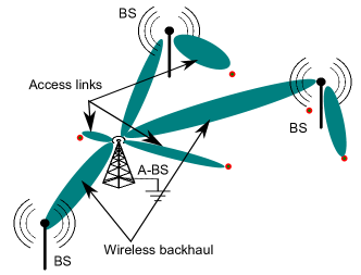
(a)

Figure 1: Self-backhauled network with the A-BS providing the wireless backhaul to the associated BSs and access link to the associated users (denoted by circles).

II-E Validation methodology

The analytical model and results presented in this paper are validated using Monte Carlo simulations employing actual building topology of two major metropolitan areas, Manhattan and Chicago [16]. The polygons representing the buildings in the corresponding regions are shown in Fig. 2. These regions represent dense urban settings, where mmWave networks are most attractive. In each simulation trial, users and BSs are dropped randomly in these geographical areas as per the corresponding densities. Users are dropped only in the outdoor regions, whereas the BSs landing inside a building polygon are assumed to be NLOS to all users. A BS-user link is assumed to be NLOS if a building blocks the line segment joining the two, and LOS otherwise. The association and propagation rules are assumed as described in the earlier sections. The specific path loss parameters used are listed in Table I and are from empirical measurements [14]. The association cells formed by two different placements of mmWave BSs in downtown Manhattan with this methodology are shown in Fig. 3.

II-F Access and backhaul load

Access and backhaul links are assumed to share (through orthogonal division) the same pool of radio resources and hence the user rate depends on the user load at BSs and BS load at A-BSs. Let ${N}_{b}$, ${N}_{u,w}$, and ${N}_{u}$ denote the number of BSs associated with the tagged A-BS, number of users served by the tagged A-BS, and the number of users associated with the tagged BS respectively. By definition, when the typical user associates with an A-BS, ${N}_{u,w}={N}_{u}$. Since an A-BS serves both users and BSs, the resources allocated to the associated BSs (which further serve their associated users) are assumed to be proportional to their average user load. Let the average number of users per BS be denoted by $\kappa\triangleq\lambda_{u}/{\lambda}$, and then the fraction of resources $\eta_{b}$ available for all the associated BSs at an A-BS are $\frac{\kappa{N}_{b}}{\kappa{N}_{b}+{N}_{u,w}}$, and those for the access link with the associated users are then $\eta_{a,w}=1-\eta_{b}=\frac{{N}_{u,w}}{\kappa{N}_{b}+{N}_{u,w}}$. The fraction of resources reserved for the associated BSs at an A-BS are assumed to be shared equally among the BSs and hence the fraction of resources available to the tagged BS from the tagged A-BS are $\eta_{b}/{N}_{b}$, which is equivalent to the resource fraction used for backhaul by the corresponding BS. The access and backhaul capacity at each BS is assumed to be shared equally among the associated users. Furthermore, the rate of a user is assumed to equal the minimum of the access link rate and backhaul link rate.

With the above described resource allocation model the rate/throughput of a user is given by (1) (at top of the page), where $\mathtt{SINR}_{a}$ corresponds to the $\mathtt{SINR}$ of the access link: $a\equiv d$ for downlink and $a\equiv u$ for uplink.

$$\Lambda_{a}((0,t])={\lambda}\pi\mathrm{C}\bigg{\{}\mathrm{D}^{2}\left[\mathrm{Q}\left(\frac{\ln(\mathrm{D}^{\alpha_{l}}/t)-m_{l}}{\sigma_{l}}\right)-\mathrm{Q}\left(\frac{\ln(\mathrm{D}^{\alpha_{n}}/t)-m_{n}}{\sigma_{n}}\right)\right]+t^{2/{\alpha_{l}}}\exp\left(2\frac{\sigma_{l}^{2}}{\alpha_{l}^{2}}+2\frac{m_{l}}{\alpha_{l}}\right)\\ \times\mathrm{Q}\left(\frac{\sigma_{l}^{2}(2/\alpha_{l})-\ln(\mathrm{D}^{\alpha_{l}}/t)+m_{l}}{\sigma_{l}}\right)+t^{2/{\alpha_{n}}}\exp\left(2\frac{\sigma_{n}^{2}}{\alpha_{n}^{2}}+2\frac{m_{n}}{\alpha_{n}}\right)\left[\frac{1}{\mathrm{C}}-\mathrm{Q}\left(\frac{\sigma_{n}^{2}(2/\alpha_{n})-\ln(\mathrm{D}^{\alpha_{n}}/t)+m_{n}}{\sigma_{n}}\right)\right]\bigg{\}}$$ (2)

II-G Hybrid networks

Co-existence with conventional UHF based $3$G and $4$G networks could play a key role in providing wide coverage, particularly in sparse deployment of mmWave networks, and reliable control channels. In this paper, a simple offloading technique is adopted wherein a user is offloaded to the UHF network if it’s $\mathtt{SINR}$ on the mmWave network drops below a threshold $\tau_{\mathrm{min}}$. Since it was shown in [27] that the aggressiveness of offloading (or the offloading bias) is proportional to the bandwidth of the orthogonal band of small cells, the proposed $\mathtt{SINR}$-based association technique is arguably reasonable for large bandwidth mmWave networks. A similar technique was also used in [32] for energy efficiency analysis.

III Rate Distribution: Downlink and Uplink

This is the main technical section of the paper, which characterizes the user rate distribution across the network in a self-backhauled mmWave network co-existing with a UHF macrocellular network.

III-A $\mathtt{SNR}$ distribution

For characterizing the downlink $\mathtt{SNR}$ distribution, the point process formed by the path loss of each BS to the typical user at origin defined as $\mathcal{N}_{a}\coloneqq\left\{L_{a}(X)=\frac{\|X\|^{\alpha}}{S}\right\}_{X\in\Phi}$, where $S\triangleq 10^{-(\chi+\beta)/10}$, on is considered. Using the displacement theorem, $\mathcal{N}_{a}$ is a Poisson process and let the corresponding intensity measure be denoted by $\Lambda_{a}(.)$.

Lemma 1.

The distribution of the path loss from the user to the tagged base station is such that ${\mathbb{P}}(L_{a}(X^{*})>t)=\exp\left(-\Lambda_{a}((0,t])\right)$, where the intensity measure is given by (2) (at top of the page), where $m_{j}=-0.1\beta_{j}\ln 10$, $\sigma_{j}=0.1\xi_{j}\ln 10$, with $j\equiv l$ for LOS and $j\equiv n$ for NLOS, and $\mathrm{Q}(.)$ is the Q-function (Standard Gaussian CCDF).

Proof.

See Appendix A. ∎

The above lemma simplifies to the scenario considered in [33] with uniform path loss exponents (i.e. no blockage) and uniform shadowing variance.

The path loss distribution for a typical backhaul link can be similarly obtained by considering the propagation process [33] $\mathcal{N}_{b}$ from A-BSs to the BS at the origin. The corresponding intensity measure $\Lambda_{b}$ is then obtained by replacing ${\lambda}$ by ${\lambda}\omega$ and replacing the access link parameters with that of backhaul link in (2).

Under the assumptions of stationary PPP for both users and BSs, considering the typical link for analysis allows characterization of the corresponding network-wide performance metric. Therefore, the $\mathtt{SNR}$ coverage defined as the distribution of $\mathtt{SNR}$ for the typical link $\mathcal{S}_{(.)}(\tau)\triangleq{\mathbb{P}^{o}}_{\Phi_{u}}(\mathtt{SNR}_{(.)}>\tau)$ is also the complementary cumulative distribution function (CCDF) of $\mathtt{SNR}$ across the entire network. The same holds for $\mathtt{SINR}$ and $\mathtt{Rate}$ coverage.

Lemma 1 enables the characterization of $\mathtt{SNR}$ distribution in a closed form in the following theorem.

Theorem 1.

The $\mathtt{SNR}$ distribution for the typical downlink, uplink, and backhaul link are respectively

$$\mathcal{S}_{d}(\tau)\triangleq{\mathbb{P}}(\mathtt{SNR}_{d}>\tau) =1-\exp\left(-{\lambda}\mathrm{M}_{a}\left(\frac{\mathrm{P}_{b}\mathrm{G_{max}}}{\tau\sigma^{2}_{N}}\right)\right)$$

$$\mathcal{S}_{u}(\tau)\triangleq{\mathbb{P}}(\mathtt{SNR}_{u}>\tau) =1-\exp\left(-{\lambda}\mathrm{M}_{a}\left(\frac{\mathrm{P}_{u}\mathrm{G_{max}}}{\tau\sigma^{2}_{N}}\right)\right)$$

$$\mathcal{S}_{b}(\tau)\triangleq{\mathbb{P}}(\mathtt{SNR}_{b}>\tau) =1-\exp\left(-{\lambda}\omega\mathrm{M}_{b}\left(\frac{\mathrm{P}_{b}\mathrm{G}^{2}_{\mathrm{max}}}{\tau\sigma^{2}_{N}}\right)\right),$$

where $\mathrm{M}_{a}(t)\triangleq\frac{\Lambda_{a}((0,t])}{{\lambda}}$ and $\mathrm{M}_{b}(t)\triangleq\frac{\Lambda_{b}((0,t])}{{\lambda}\omega}$.

Proof.

For the downlink case,

$${\mathbb{P}}(\mathtt{SNR}_{d}>\tau) ={\mathbb{P}}\left(\frac{\mathrm{P}_{b}\mathrm{G_{max}}L_{a}(X^{*})^{-1}}{\sigma^{2}_{N}}>\tau\right)$$

$$=1-\exp\left(-{\lambda}\mathrm{M}_{a}\left(\frac{\mathrm{P}_{b}\mathrm{G_{max}}}{\tau\sigma^{2}_{N}}\right)\right),$$

where the last equality follows from Lemma 1. Uplink and backhaul link coverage follow similarly. ∎

Noting the dependence of $\Lambda_{(.)}(t)$ on $t$ and ${\lambda}$, the $\mathtt{SNR}$ coverage (both access and backhaul) are directly proportional to the densities, power, and antenna gain of the respective links.

As it can be noted, users are assumed to be transmitting with maximum power in the uplink (without power control) in the above derivation. This is arguably reasonable as the uplink $\mathtt{SNR}$ is already problematic in mmWave networks, even with max power transmission. However, the uplink $\mathtt{SNR}$ derivation above can be extended to incorporate uplink fractional power control employed in LTE networks, as shown in Appendix B.

III-B Interference in mmWave networks

This section provides an analytical treatment of interference in mmWave networks. In particular, the focus of this section is to upper bound the interference-to-noise ($\mathtt{INR}$) distribution (hence provide more insight into an earlier comment of noise-limited nature ($\mathtt{SNR}\approx\mathtt{SINR}$) of mmWave networks), and quantify the impact of key design parameters on this upper bound. Without any loss of generality, each BS is assumed to be an A-BS (i.e. $\omega=1$) in this section and hence the subscript ‘a’ for access is dropped.

$$\mathrm{M}^{\prime}(t)\triangleq\frac{\mathrm{d}\mathrm{M}(t)}{\mathrm{d}t}=\pi\mathrm{C}\Bigg{\{}\frac{\mathrm{D}^{2}}{\sqrt{2\pi}t}\left[\frac{1}{\sigma_{l}}\exp\left(-\left(\frac{\ln(\mathrm{D}^{\alpha_{l}}/t)-m_{l}}{\sqrt{2\sigma_{l}^{2}}}\right)^{2}\right)-\frac{1}{\sigma_{n}}\exp\left(-\left(\frac{\ln(\mathrm{D}^{\alpha_{n}}/t)-m_{n}}{\sqrt{2\sigma_{n}^{2}}}\right)^{2}\right)\right]+\\ \exp\left(2\frac{\sigma_{l}^{2}}{\alpha_{l}^{2}}+2\frac{m_{l}}{\alpha_{l}}\right)t^{\frac{2}{\alpha_{l}}-1}\left[\frac{2}{\alpha_{l}}\mathrm{Q}\left(\frac{\sigma_{l}^{2}(2/\alpha_{l})-\ln(\mathrm{D}^{\alpha_{l}}/t)+m_{l}}{\sigma_{l}}\right)-\frac{1}{\sqrt{2\pi\sigma_{l}^{2}}}\exp\left(-\left(\frac{\sigma_{l}^{2}(2/\alpha_{l})-\ln(\mathrm{D}^{\alpha_{l}}/t)+m_{l}}{\sqrt{2\sigma_{l}^{2}}}\right)^{2}\right)\right]+\\ \exp\left(2\frac{\sigma_{n}^{2}}{\alpha_{n}^{2}}+2\frac{m_{n}}{\alpha_{n}}\right)t^{\frac{2}{\alpha_{n}}-1}\left[\frac{2}{\mathrm{C}\alpha_{n}}-\frac{2}{\alpha_{n}}\mathrm{Q}\left(\frac{\sigma_{n}^{2}(2/\alpha_{n})-\ln(\mathrm{D}^{\alpha_{n}}/t)+m_{n}}{\sigma_{n}}\right)+\frac{1}{\sqrt{2\pi\sigma_{n}^{2}}}\exp\left(-\left(\frac{\sigma_{n}^{2}(2/\alpha_{n})-\ln(\mathrm{D}^{\alpha_{n}}/t)+m_{n}}{\sqrt{2\sigma_{n}^{2}}}\right)^{2}\right)\right]\Bigg{\}}.$$ (4)

Consider the sum over the earlier defined PPP $\mathcal{N}$

$$I_{t}\triangleq\sum_{Y\in\mathcal{N}}Y^{-1}K_{Y},$$ (3)

where $K_{Y}$ are i.i.d. marks associated with $Y\in\mathcal{N}$. For example, if $K_{Y}=\mathrm{P}_{b}\psi_{Y}$ with $\psi_{Y}$ being the random antenna gain on the link from $Y$, then $I_{t}$ denotes the total received power from all BSs at the typical user. The following proposition provides an upper bound to downlink $\mathtt{INR}$ in mmWave networks.

Proposition 1.

The CCDF of $\mathtt{INR}$ is upper bounded as

$${\mathbb{P}}(\mathtt{INR}>y)\leq\frac{2e^{a\sigma^{2}_{N}y}}{\pi}\int_{0}^{\infty}\mathrm{Re}(\bar{\mathcal{L}_{I_{t}}}(a+iu))\cos(u\sigma^{2}_{N}y)\mathrm{d}u,$$

where $\bar{\mathcal{L}_{I_{t}}}(z)=1/z-\mathcal{L}_{I_{t}}(z)/z$ with

$$\mathcal{L}_{I_{t}}(z)=\exp\left(-{\lambda}{\mathbb{E}\left[{zK\int_{u>0}\frac{1-\exp(-u)}{u^{2}}\mathrm{M}^{\prime}\left(\frac{zK}{u}\right)\mathrm{d}u}\right]}\right)$$

and $\mathrm{M}^{\prime}$ is given by (4) (at top of the page).

Proof:

The downlink interference $I_{d}=I_{t}-K_{X^{*}}/X^{*}$ is clearly upper bounded by $I_{t}$ and hence $\mathtt{INR}\triangleq I_{d}/\sigma^{2}_{N}$ has the property: ${\mathbb{P}}(\mathtt{INR}>y)\leq{\mathbb{P}}(I_{t}>\sigma^{2}_{N}y)$. The sum in (3) is the shot noise associated with $\mathcal{N}$ and the corresponding Laplace transform is represented as the Laplace functional of the shot noise of $\mathcal{N}$, $\mathcal{L}_{I_{t}}(z)\triangleq{\mathbb{E}\left[{\exp(-zI_{t})}\right]}$

$$=\exp\left(-{\mathbb{E}_{K}\left[{\int_{y>0}\left\{1-\exp(-zK/y)\right\}\Lambda(\mathrm{d}y)}\right]}\right),$$

and the Laplace transform associated with the CCDF of the shot noise is $\bar{\mathcal{L}_{I_{t}}}(z)=1/z-\mathcal{L}_{I_{t}}(z)/z$. The CCDF of the shot noise can then be obtained from the corresponding Laplace transform using the Euler characterization [34]

$$\bar{F}_{I_{t}}(y)\triangleq{\mathbb{P}}(I_{t}>y)=\frac{2e^{ay}}{\pi}\int_{0}^{\infty}\mathrm{Re}(\bar{\mathcal{L}_{I_{t}}}(a+iu))\cos uy\mathrm{d}u.$$

∎

The interference on the uplink is generated by users transmitting on the same radio resource as the typical user. Assuming each BS gives orthogonal resources to users associated with it, one user per BS would interfere with the uplink transmission of the typical user. The point process of the interfering users, for the analysis in this section, is assumed to be a PPP $\Phi_{u,b}$ of intensity same as that of BSs, i.e., ${\lambda}$. In the same vein as the above discussion, the propagation process $\mathcal{N}_{u}\coloneqq\{L_{a}(X)\}_{X\in\Phi_{u,b}}$ captures the propagation loss from users to the BS under consideration at origin. The shot noise $I_{t}\triangleq\sum_{U\in\mathcal{N}_{u}}U^{-1}K_{U}$ then upper bounds the uplink interference with $K_{U}=\mathrm{P}_{u}\psi_{U}$.

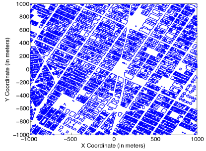
(a) Manhattan

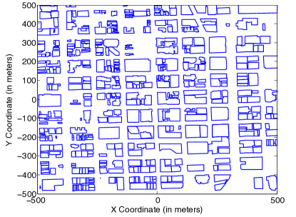
(b) Chicago

Figure 2: Building topology of Manhattan and Chicago used for validation.

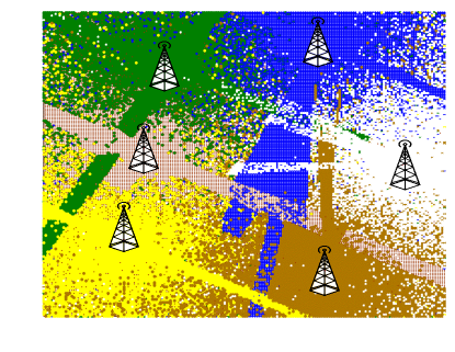
(a)

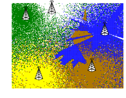
(b)

Figure 3: Association cells in different shades and colors for two different BS placement in Manhattan region. Noticeable discontinuity and irregularity of the cells show the sensitivity of path loss to blockages and the dense building topology (shown in Fig. 2a).

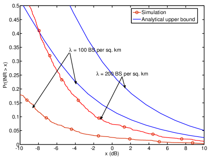
(a)

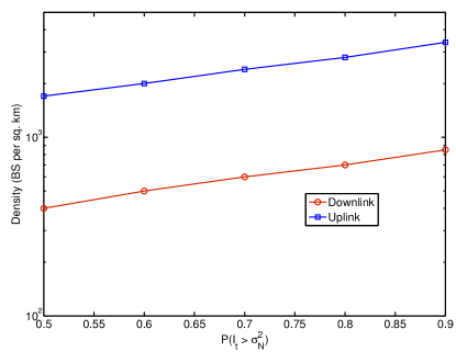
(b)

Figure 4: (a) Total power to noise ratio and $\mathtt{INR}$ for the proposed model, and (b) the variation of the density required for the total power to exceed noise with a given probability.

The analytical total power to noise ratio bound for the downlink with the parameters of Table I is shown in Fig. 4a. The Matlab code for computing the upper bound is available online [35]. Also shown is the corresponding $\mathtt{INR}$ obtained through simulations. As can be observed from the analytical upper bounds and simulation, the interference power does not dominate noise power for the large bandwidth and narrow beam-width network considered here. In fact, $\mathtt{INR}>0$ dB is observed in less than $20\%$ of the cases even at high base station densities of about $200$ per sq. km. As a consequence of the stochastic dominance, the distribution of the total power (derived above) can be used to lower bound the density required for interference to dominate noise. The minimum BS density required for achieving a given ${\mathbb{P}}(I_{t}>\sigma^{2}_{N})$ for uplink and downlink is shown in Fig. 4b. As can be seen, a density of at least $500$ and $2000$ BS per sq. km is required for guaranteeing downlink and uplink interference to exceed noise power with $0.7$ probability, respectively. In general, the $\mathtt{INR}$ distribution depends on the bandwidth, antenna directivity (beam-width), carrier frequency, and density. The following corollary quantifies this effect.

Corollary 1.

Density-Directivity-Bandwidth-Frequency Equivalence. In the case of uniform path loss exponent ($\alpha_{l}=\alpha_{n}=\alpha$) and shadowing variance for all links, the upper bound to the $\mathtt{INR}$ is proportional to $\frac{{\lambda}\mathrm{P}^{2/\alpha}{\mathbb{E}\left[{\psi^{2/\alpha}}\right]}}{\nu^{4/\alpha}\mathrm{B}^{2/\alpha}}.$

Proof.

For the special case of uniform path loss exponent and shadowing variance for all links, $\mathrm{M}(u)=\pi{\mathbb{E}\left[{S^{2/\alpha}}\right]}u^{2/\alpha}$ and $\mathrm{M}^{\prime}(u)=\frac{2\pi}{\alpha}{\mathbb{E}\left[{S^{2/\alpha}}\right]}u^{2/\alpha-1}$, the Laplace transform of $I_{t}$ is

$$\mathcal{L}_{I_{t}}(z) =\exp\left(2\pi\frac{{\lambda}}{\alpha}z^{2/\alpha}\mathrm{P}^{2/\alpha}{\mathbb{E}\left[{S^{2/\alpha}}\right]}{\mathbb{E}\left[{\psi^{2/\alpha}}\right]}\Gamma\left(\frac{-2}{\alpha}\right)\right),$$

and the Laplace transform of $I_{t}/\sigma^{2}_{N}$ is

$$\exp\left(2\pi\frac{{\lambda}}{\alpha}\left(\frac{z}{\sigma^{2}_{N}}\right)^{2/\alpha}\mathrm{P}^{2/\alpha}{\mathbb{E}\left[{S^{2/\alpha}}\right]}{\mathbb{E}\left[{\psi^{2/\alpha}}\right]}\Gamma\left(\frac{-2}{\alpha}\right)\right).$$

Noting the dependence of thermal noise power $\sigma^{2}_{N}$ on bandwidth and that of ${\mathbb{E}\left[{S^{2/\alpha}}\right]}$ on free space path loss (and thus on the carrier frequency) leads to the final result. ∎

From the above corollary, it can be noted that the upper bound on the $\mathtt{INR}$ distribution is invariant with increase in BS density or beam-width if the bandwidth and/or carrier frequency also scale appropriately.

The $\mathtt{SINR}$ distribution of the typical link defined as $\mathcal{P}_{(.)}(\tau)\triangleq{\mathbb{P}^{o}}_{\Phi_{u}}(\mathtt{SINR}_{(.)}>\tau)$ can be derived using the intensity measure of Lemma 1 and is delegated to Appendix C. However, as shown in this section, $\mathtt{SNR}$ provides a good approximation to $\mathtt{SINR}$ for directional large bandwidth mmWave networks in densely blocked settings (typical for urban settings), and hence the following analysis will, deliberately, ignore interference (i.e. $\mathcal{P}\approx\mathcal{S}$). However, the corresponding simulation results include interference, thereby validating this assumption. For an interference-limited setting, the analytical rate distribution results can be obtained by replacing $\mathcal{S}$ with $\mathcal{P}$.

III-C Load characterization

As mentioned earlier, throughput on access and backhaul link depends on the number of users sharing the access link and the number of BSs backhauling to the same A-BS respectively. Hence there are two types of association cells in the network: 1. user association cell of a BS – the region in which all users are served by the corresponding BS, and 2. BS association cell of an A-BS – the region in which all BSs are served by that A-BS. Formally, the user association cell of a BS (or an A-BS) located at $X\in 2$ is

$$\mathcal{C}_{X}\triangleq\left\{Y\in 2:L_{a}(X,Y)<L_{a}(T,Y)\,\,\forall\,T\in\Phi\right\}$$

and the BS association cell of an A-BS located at $Z\in 2$

$$\mathcal{C}_{w,Z}\triangleq\left\{Y\in 2:L_{b}(Z,Y)<L_{b}(T,Y)\,\,\forall\,T\in\Phi_{w}\right\}.$$

Due to the complex associations cells in such networks, the resulting distribution of the association areas (required for characterizing load distribution) is highly non-trivial to characterize exactly. The corresponding means, however, are characterized exactly by the following remark.

Remark 1.

Mean Association Areas. Under the modeling assumptions of Sec. II, the minimum path loss association rule corresponds to a stationary (translation invariant) association [36], and consequently the mean user association area of a typical BS equals the inverse of the corresponding density, i.e., $\mathbb{E}^{o}_{\Phi}\left[|\mathcal{C}_{0}|\right]=\frac{1}{{\lambda}}$, and the mean BS association area of a typical A-BS equals $\mathbb{E}^{o}_{\Phi_{w}}\left[|\mathcal{C}_{w,0}|\right]=\frac{1}{{\lambda}\omega}$. Furthermore, the area distribution of the tagged BS and A-BS follow an area biased distribution as compared to that of the corresponding typical areas resulting in the corresponding means to be ${\lambda}\mathbb{E}^{o}_{\Phi}\left[|\mathcal{C}_{0}|^{2}\right]$ and ${\lambda}\omega\mathbb{E}^{o}_{\Phi_{w}}\left[|\mathcal{C}_{w,0}|^{2}\right]$ respectively.

The above remark highlights that, although association regions are structurally very different from a distance-based Poisson-Voronoi (PV), they have the same mean areas as that of the PV with regards to the typical cell. This leads to the next approximation.

Assumption 1.

Association area distribution. The association area distribution of a typical BS and that of a typical A-BS is assumed to be same as that of the area distribution of a typical PV with the same mean area (i.e. same density).

The above approximation was proposed in [27] for approximating area distribution of weighted PV and was verified through simulations. This approximation is validated in subsequent sections using simulations in the context of rate distribution in mmWave networks. The probability mass function (PMF) of the resulting loads based on the above discussion are stated below. The proofs follow along the similar lines of [27, 37] and are thus omitted.

Proposition 2.

1. The PMF of the number of users ${N}_{u}$ associated with the tagged BS is

   $$\mathsf{K}_{t}(\lambda_{u},{\lambda},n)={\mathbb{P}}\left({N}_{u}=n\right),\,\,\,\\ n\geq 1,$$

   where

   $$\mathsf{K}_{t}(c,d,n)=\frac{3.5^{3.5}}{(n-1)!}\frac{\Gamma(n+3.5)}{\Gamma(3.5)}\left(\frac{c}{d}\right)^{n-1}\left(3.5+\frac{c}{d}\right)^{-(n+3.5)},$$

   and $\Gamma(x)=\int_{0}^{\infty}\exp(-t)t^{x-1}\mathrm{d}t$ is the gamma function. The corresponding mean is $\bar{N}_{u}\triangleq{\mathbb{E}\left[{{N}_{u}}\right]}=1+1.28\frac{\lambda_{u}}{{\lambda}}$ [27]. When the user associates with an A-BS ${N}_{u,w}={N}_{u}$. Otherwise, the number of users ${N}_{u,w}$ served by the tagged A-BS follow the same distribution as those in a typical BS given by

   $$\mathsf{K}(\lambda_{u},{\lambda},n)={\mathbb{P}}\left({N}_{u,w}=n\right),\,\,\,\\ n\geq 0,$$

   where

   $$\mathsf{K}(c,d,n)=\frac{3.5^{3.5}}{n!}\frac{\Gamma(n+3.5)}{\Gamma(3.5)}\left(\frac{c}{d}\right)^{n}\left(3.5+\frac{c}{d}\right)^{-(n+3.5)}.$$

   The corresponding mean is $\bar{N}_{u,w}\triangleq{\mathbb{E}\left[{{N}_{u,w}}\right]}=\frac{\lambda_{u}}{{\lambda}}$.

2. The number of BSs ${N}_{b}$ served by the tagged A-BS, when the typical user is served by the A-BS, has the same distribution as the number of BSs associated with a typical A-BS and hence

   $$\mathsf{K}({\lambda}(1-\omega),{\lambda}\omega,n)={\mathbb{P}}\left({N}_{b}=n\right),\,\,\\ n\geq 0.$$

   The corresponding mean is $\bar{N}_{b}\triangleq{\mathbb{E}\left[{{N}_{b}}\right]}=\frac{1-\omega}{\omega}$. In the scenario where the typical user associates with a BS, the number of BSs ${N}_{b}$ associated with the tagged A-BS is given by

   $$\mathsf{K}_{t}({\lambda}(1-\omega),\omega{\lambda},n)={\mathbb{P}}\left({N}_{b}=n\right),\,\,\\ n\geq 1.$$

   The corresponding mean is $\bar{N}_{b}=1+1.28\frac{1-\omega}{\omega}$.

$$\mathcal{R}(\rho)\triangleq{\mathbb{P}}(\mathtt{Rate}>\rho)=\omega\sum_{n\geq 0,m\geq 1}\mathsf{K}({\lambda}(1-\omega),{\lambda}\omega,n)\mathsf{K}_{t}(\lambda_{u},{\lambda},m)\mathcal{S}_{d}\left(v\{\hat{\rho}(\kappa n+m)\}\right)$$

$$+(1-\omega)\sum_{l\geq 1,n\geq 1,m\geq 0}\mathsf{K}_{t}(\lambda_{u},{\lambda},l)\mathsf{K}_{t}({\lambda}(1-\omega),\omega{\lambda},n)\mathsf{K}(\lambda_{u},{\lambda},m)\mathcal{S}_{b}\left(v\left\{\hat{\rho}l(n+m/\kappa)\right\}\right)\mathcal{S}_{d}\left(v\left\{\hat{\rho}l\frac{n+m/\kappa}{n+m/\kappa-1}\right\}\right)$$ (5)

$$\bar{\mathcal{R}}(\rho)=\omega\mathcal{S}_{d}\left(v\left\{\hat{\rho}\left(\frac{\lambda_{u}(1-\omega)}{{\lambda}\omega}+1+1.28\frac{\lambda_{u}}{{\lambda}}\right)\right\}\right)\\ +(1-\omega)\mathcal{S}_{b}\left(v\left\{\hat{\rho}\left(1+1.28\frac{\lambda_{u}}{{\lambda}}\right)\left(2+1.28\frac{1-\omega}{\omega}\right)\right\}\right)\mathcal{S}_{d}\left(v\left\{\hat{\rho}\left(1+1.28\frac{\lambda_{u}}{{\lambda}}\right)\frac{2+1.28(1-\omega)/\omega}{1+1.28(1-\omega)/\omega}\right\}\right)$$ (6)

III-D Rate coverage

As emphasized in the introduction, the rate distribution (capturing the impact of loads on access and backhaul links) is vital for assessing the performance of self-backhauled mmWave networks. The lemmas below characterize the downlink rate distribution for a mmWave and a hybrid network employing the following approximations. Corresponding results for the uplink are obtained by replacing $\mathcal{S}_{d}$ with $\mathcal{S}_{u}$.

Assumption 2.

The number of users ${N}_{u}$ served by the tagged BS and the number of BSs ${N}_{b}$ served by the tagged A-BS are assumed independent of each other and the corresponding link $\mathtt{SINR}$s/$\mathtt{SNR}$s.

Assumption 3.

The spectral efficiency of the tagged backhaul link is assumed to follow the same distribution as that of the typical backhaul link.

Lemma 2.

The rate coverage of a typical user in a self backhauled mmWave network, described in Sec. II, for a rate threshold $\rho$ is given by (III-C) (at top of the page), where $\hat{\rho}=\rho/\mathrm{B}$, $v(x)=2^{x}-1$, and $\mathcal{S}_{(.)}$ are from Theorem 1.

Proof.

Let $\mathcal{A}_{w}$ denote the event of the typical user associating with an A-BS, i.e., ${\mathbb{P}}(\mathcal{A}_{w})=\omega$. Then, using (1), the rate coverage is

$$\mathcal{R}(\rho)=\omega{\mathbb{P}}\left(\frac{\eta_{a,w}}{{N}_{u,w}}\log(1+\mathtt{SINR}_{d})>\hat{\rho}|\mathcal{A}_{w}\right)+(1-\omega)\times$$

$${\mathbb{P}}\left(\frac{1}{{N}_{u}}\min\left(\left(1-\frac{\eta_{b}}{{N}_{b}}\right)\log(1+\mathtt{SINR}_{d}),\frac{\eta_{b}}{{N}_{b}}\log(1+\mathtt{SINR}_{b})\right)>\hat{\rho}|\bar{\mathcal{A}_{w}}\right)$$

$$=\omega{\mathbb{E}\left[{\mathcal{S}_{d}(v(\hat{\rho}\left\{{N}_{u,w}+\kappa{N}_{b}\right\}))}\right]}+(1-\omega)\times$$

$${\mathbb{E}\left[{\mathcal{S}_{d}\left(v\left\{\hat{\rho}{N}_{u}\frac{{N}_{b}+{N}_{u,w}/\kappa}{{N}_{b}+{N}_{u,w}/\kappa-1}\right\}\right)\mathcal{S}_{b}(v\{\hat{\rho}{N}_{u}({N}_{b}+{N}_{u,w}/\kappa)\})}\right]}.$$

The rate coverage expression then follows by invoking the independence among various loads and $\mathtt{SNR}$s. ∎

In case the different loads in the above lemma are approximated with their respective means, the rate coverage expression is simplified as in the following corollary.

Corollary 2.

The rate coverage with mean load approximation using Proposition 2 is given by (6) (at top of the page).

As can be observed from the above corollary, increasing the fraction of A-BSs $\omega$ in the network increases the probability of being served by an A-BS (the weight of the first term). The rate from an A-BS ($\mathcal{S}_{d}(.)$ in the first term) also increases with $\omega$, as user and BS load per A-BS decreases. Furthermore, increasing $\omega$ also increases the backhaul rate ($\mathcal{S}_{b}(.)$ in the second term) of a user associated with a BS. Further investigation into the interplay of ${\lambda}$, $\omega$, and rate is deferred to Sec. IV-D.

Remark 2.

In practical communications systems, it might be unfeasible to transmit reliably with any modulation and coding (MCS) below a certain $\mathtt{SNR}$: $\tau_{0}$ (say), and in that case $\mathtt{Rate}=0$ for $\mathtt{SNR}<\tau_{0}$. Such a constraint can be incorporated in the above analysis by replacing $v\to\max(v,\tau_{0})$.

The following lemma characterizes the rate distribution in a hybrid network with the association technique of Sec. II-G.

Lemma 3.

The rate distribution in a hybrid mmWave network (with $\omega=1$) co-existing with a UHF macrocellular network, described in Sec. II-G, is

$$\mathcal{R}_{H}(\rho)=\mathcal{R}_{1}(\rho)+(1-\mathcal{S}_{d}(\tau_{\mathrm{min}}))\\ \times\sum_{n\geq 1}\mathsf{K}_{t}(\lambda_{u}-\lambda_{u,m},\mu,n)\mathcal{P}_{\mu}(v\left\{\rho n/\mathrm{B}_{\mu}\right\}),$$

where $\mathcal{R}_{1}(\rho)$ is obtained from Lemma 2 by replacing $\lambda_{u}\to\lambda_{u,m}\triangleq\lambda_{u}\mathcal{S}_{d}(\tau_{\mathrm{min}})$ (the effective density of users associated with mmWave network) and $v\to v_{1}\triangleq\max(v,\tau_{\mathrm{min}})$, $\mathcal{P}_{\mu}$ is the $\mathtt{SINR}$ coverage on UHF network, and $\mathsf{K}_{t}(\lambda_{u}-\lambda_{u,m},\mu,n)$ is the PMF of the number of users ${N}_{\mu}$ associated with the tagged UHF BS.

Proof.

Under the association method of Sec. II-G, the rate coverage in the hybrid setting is

$${\mathbb{P}}(\mathtt{Rate}>\rho) ={\mathbb{P}}(\mathtt{Rate}>\rho\cap\mathtt{SINR}_{d}>\tau_{\mathrm{min}})$$

$$+{\mathbb{P}}(\mathtt{Rate}>\rho\cap\mathtt{SINR}_{d}<\tau_{\mathrm{min}})$$

$$=\mathcal{R}_{1}(\rho)+(1-\mathcal{S}_{d}(\tau_{\mathrm{min}})){\mathbb{E}\left[{\mathcal{P}_{\mu}(v\left\{\rho/\mathrm{B}_{\mu}{N}_{\mu}\right\})}\right]},$$

where the first term on the RHS is the rate coverage when associated with the mmWave network and hence $\mathcal{R}_{1}$ follows from the previous Lemma 2 by incorporating the offloading $\mathtt{SINR}$ threshold and reducing the user density to account for the users offloaded to the macrocellular network (fraction $1-\mathcal{S}_{d}(\tau_{\mathrm{min}})$). The second term is the rate coverage when associated with the UHF network and ${N}_{\mu}$ is the load on the tagged UHF BS, whose distribution can be expressed as in [27] noting the mean association cell area of a UHF BS is $\frac{1-\mathcal{S}_{d}(\tau_{\mathrm{min}})}{\mu}$. The UHF network’s $\mathtt{SINR}$ coverage $\mathcal{P}_{\mu}$ can be derived as in earlier work [33, 38]. ∎

III-E Validation

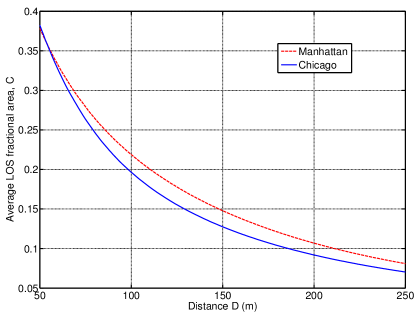
Figure 5: Average LOS fractional area as a function of radius $\mathrm{D}$ averaged over the respective geographical regions.

In the proposed model, the primary geography dependent parameters are $\mathrm{C}$ and $\mathrm{D}$. As mentioned earlier, for a given $\mathrm{D}$, the parameter $\mathrm{C}$ is the average LOS fractional area in a disk of radius $\mathrm{D}$. In order to fit the proposed model to a particular geographical region, the following methodology is adopted. Using Monte Carlo simulations in the setup of Sec. II-E, the average fraction of LOS area in a disk of radius $\mathrm{D}$ around randomly dropped users is obtained as a function of the radius $\mathrm{D}$. Fig. 5 shows the empirical $\mathrm{C}$ obtained by averaging over the Manhattan and Chicago regions of Fig. 2.

TABLE II: Values of $\mathrm{D}$ and $\mathrm{C}$

Urban area	$\mathrm{D}$ (m)	$\mathrm{C}$
Chicago	250	0.07
Manhattan	200	0.11

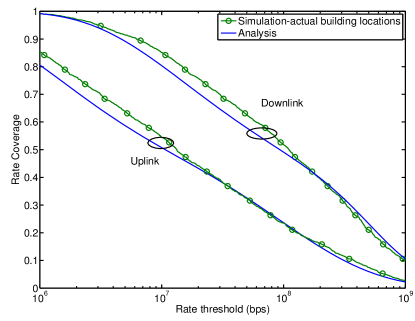
(a) Manhattan

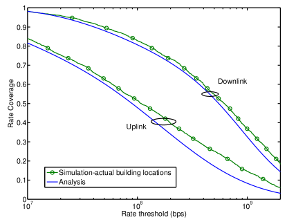
(b) Chicago

Figure 6: Downlink rate distribution comparison from simulation and analysis for BS density $30$ per sq. km in Manhattan (a) and $60$ per sq. km in Chicago (b) with user density of $200$ per sq. km.

The downlink rate distribution (both uplink and downlink) obtained from simulations (as per Sec. II-E) and analysis (Lemma 2) is shown in Fig. 6 for the two cities with two different different BS densities and user density of $200$ per sq. km. The parameters ($\mathrm{C}$, $\mathrm{D}$) used in analysis for the specific geography are obtained using Fig. 5 and are given in Table II. The closeness of the analytical results to those of the simulations validates (a) the ability of the proposed simple blockage model to capture the blockage characteristics of dense urban settings, and (b) the load characterization for irregular association cells (Fig. 3) in a mmWave network. The closeness of the match builds confidence in the model and the derived design insights.

In the above plots any ($\mathrm{C}$, $\mathrm{D}$) pair from Fig. 5 can be used. However, it is observed that the match is better for the ($\mathrm{C}$, $\mathrm{D}$) pair with larger $\mathrm{D}$ ($200$-$250$m, see [16] for robustness analysis). This is due to the fact that the LOS fractional area ($\mathrm{C}_{\bar{\mathrm{D}}}$, say) beyond distance $\mathrm{D}$ is ignored, which is a better approximation for larger $\mathrm{D}$. It is straightforward to allow LOS area outside $\mathrm{D}$ in the analysis (as shown in Appendix A) but estimating the same using actual building locations is quite computationally intensive and tricky, as averaging needs to be done over a considerably larger area. The fit procedure is simplified, though not sacrificing the accuracy of the fit much (as seen), by setting $\mathrm{C}_{\bar{\mathrm{D}}}=0$ in the model.

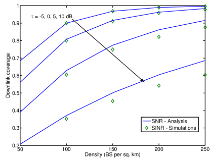
(a) Downlink

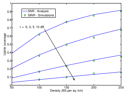
(b)

Figure 7: Comparison of $\mathtt{SINR}$ (analysis) and $\mathtt{SINR}$ (simulation) coverage with varying BS density.

IV Performance analysis and trends

IV-A Coverage and density

The downlink and uplink coverage for various thresholds and density of BSs is shown in Fig. 7. There are two major observations:

• The analytical $\mathtt{SNR}$ tracks the $\mathtt{SINR}$ obtained from simulation quite well for both downlink and uplink. A small gap ($<10\%$) is observed for an example downlink case with larger BS density ($250$ per sq. km) and a higher threshold of $10$ dB.

• Increasing the BS density improves both the downlink and uplink coverage and hence the spectral efficiency – a trend in contrast to conventional interference-limited networks, which are nearly invariant in $\mathtt{SINR}$ to density.

As seen in Sec. III-B, interference is expected to dominate the thermal noise for very large densities. The trend for downlink $\mathtt{SINR}$ coverage (derived in Appendix C assuming exponential fading power gain) for such densities is shown in Fig. 8 for lightly ($\mathrm{C}=0.5$) and densely blocked ($\mathrm{C}=0.11$) scenarios. All BSs are assumed to be transmitting in Fig. 8a, whereas BSs only with a user in the corresponding association cell are assumed to be transmitting in Fig. 8b. The coverage for the latter case is obtained by thinning the interference field by probability $1-\mathsf{K}(\lambda_{u},{\lambda},0)$ (details in Appendix C). As can be seen, ignoring the finite user population, the $\mathtt{SINR}$ coverage saturates, where that saturation is achieved quickly for lightly blocked scenarios–a trend corroborated by the observations of [24]. However, accounting for the finite user population leads to a different trend, as the increasing density monotonically improves the path loss to the tagged BS, but the interference is (implicitly) capped by the finite user density of $1000$ per sq. km.

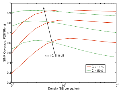
(a) All BSs transmit

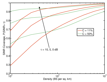
(b) BSs with an active user transmit

Figure 8: $\mathtt{SINR}$ coverage variation with large densities for different blockage densities.

IV-B Rate coverage

The variation of downlink and uplink rate distribution with the density of infrastructure for a fixed A-BS fraction $\omega=0.5$ is shown in Fig 9. Reducing the cell size by increasing density boosts the coverage and decreases the load per base station. This dual benefit improves the overall rate drastically with density as shown in the plot. Further, the good match of analytical curves to that of simulation also validates the analysis for uplink and downlink rate coverage.

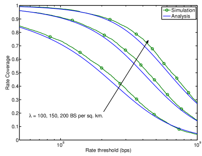
(a) Downlink

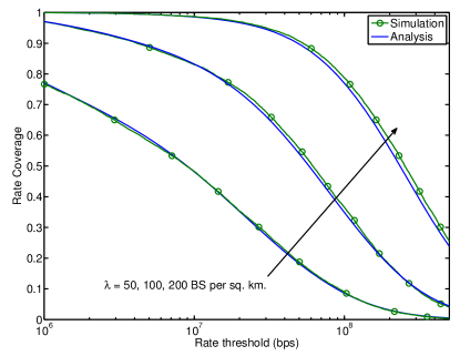
(b) Uplink

Figure 9: Downlink and uplink rate coverage for different BS densities and fixed $\omega=0.5$.

The variation in rate distribution with bandwidth is shown in Fig. 10 for a fixed BS density ${\lambda}=100$ BS per sq. km and $\omega=1$. Two observations can be made here: 1) median and peak rate increase considerably with the availability of larger bandwidth, whereas 2) cell edge rates exhibit a non-increasing trend. The latter trend is due to the low $\mathtt{SNR}$ of the cell edge users, where the gain from bandwidth is counterbalanced by the loss in $\mathtt{SNR}$. Further, if the constraint of $\mathtt{Rate}=0$ for $\mathtt{SNR}<\tau_{0}$ is imposed, cell edge rates would actually decrease as shown in Fig. 10b due to the increase in ${\mathbb{P}}(\mathtt{SNR}<\tau_{0})$, highlighting the impossibility of increasing rates for power-limited users in mmWave networks by just increasing the system bandwidth. In fact, it may be counterproductive.

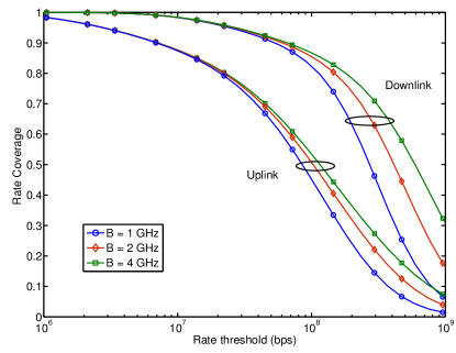
(a) $\tau_{0}=0$

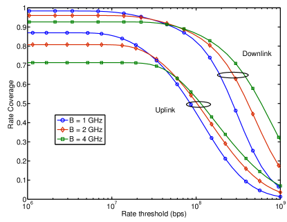
(b) $\tau_{0}=0.1$

Figure 10: Effect of bandwidth and min $\mathtt{SNR}$ constraint ($\mathtt{Rate}=0$ for $\mathtt{SNR}<\tau_{0}$) on rate distribution for BS density $100$ per sq. km.

IV-C Impact of co-existence

The rate distribution of a mmWave only network and that of a mmWave-UHF hybrid network is shown in Fig. 11 for different mmWave BS densities and fixed UHF network density of $\mu=5$ BS per sq. km. The path loss exponent for the UHF link is assumed to equal $4$ with lognormal shadowing of $8$ dB standard deviation. Offloading users from mmWave to UHF, when the link $\mathtt{SNR}$ drops below $\tau_{\mathrm{min}}=-10$ dB improves the rate of edge users significantly, when the min $\mathtt{SNR}$ constraint ($\tau_{0}=-10$ dB) is imposed. Such gain from co-existence, however, reduces with increasing mmWave BS density, as the fraction of “poor” $\mathtt{SNR}$ users reduces. Without any such minimum $\mathtt{SNR}$ consideration, i.e., $\tau_{0}=0$, mmWave is preferred due to the $100$x larger bandwidth. So the key takeaway here is that users should be offloaded to a co-existing UHF macrocellular network only when reliable communication over the mmWave link is unfeasible.

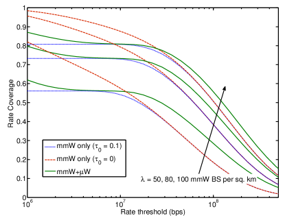
Figure 11: Downlink rate distribution for mmWave only and hybrid network for different mmWave BS density and fixed UHF density of 5 BS per sq. km.

IV-D Impact of self-backhauling

The variation of downlink rate distribution with the fraction of A-BSs $\omega$ in the network with BS density of $100$ and $150$ per sq. km is shown in Fig. 12. As can be seen, providing wired backhaul to increasing fraction of BSs improves the overall rate distribution. However “diminishing return” is seen with increasing $\omega$ as the bottleneck shifts from the backhaul to the air interface rate. Further, it can be observed from the plot that different combinations of A-BS fraction and BS density, e.g. ($\omega=0.25$, $\lambda=150$) and ($\omega=0.5$, $\lambda=100$) lead to similar rate distribution. This is investigated further using Lemma 2 in Fig. 13, which characterizes the different contours of ($\omega$, ${\lambda}$) required to guarantee various median rates $\rho_{50}$ ($\mathcal{R}(\rho_{50})=0.5$) in the network. For example, a median rate of $400$ Mbps in the network can be provided by either $\omega=0.9,{\lambda}=110$ or $\omega=0.3,{\lambda}=200$. Thus, the key insight from these results is that it is feasible to provide the same QoS (median rate here) in the network by either providing wired backhaul to a small fraction of BSs in a dense network, or by increasing the corresponding fraction in a sparser network.

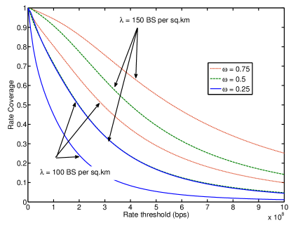
Figure 12: Rate distribution with variation in $\omega$

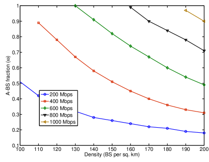
Figure 13: The required $\omega$ for achieving different median rates with varying density

In the above plots, the actual number of A-BSs in a given area increased with increasing density for a fixed $\omega$, but if the density of A-BSs is fixed ($\gamma$, say) while increasing the density of BSs, i.e., $\omega=\frac{\gamma}{{\lambda}}$ for some constant $\gamma$, would a similar trend as the earlier plot be seen? This can be answered by a closer look at Lemma 2. With increasing ${\lambda}$, the rate coverage of the access link increases shifting the bottleneck to backhaul link, which in turn is limited by the A-BS density. This notion is formalized in the following proposition.

Proposition 3.

We define the saturation density ${\lambda}_{\mathrm{sat}}^{\delta}(\gamma)$ as the density beyond which only marginal ($\delta\%$ at most) gain in rate coverage can be obtained with A-BS density fixed at $\gamma$, and characterized as

$$\arg\inf_{{\lambda}}\left\{\|\mathcal{S}_{d}\left(v\left\{\hat{\rho}1.28\frac{\lambda_{u}}{{\lambda}}\right\}\right)-1\|\leq\delta/\mathcal{S}_{b}\left(v\left\{\hat{\rho}1.28^{2}\frac{\lambda_{u}}{\gamma}\right\}\right)\right\}.$$ (7)

Proof.

As the contribution from the access rate coverage can be at most $1$, the saturation density is characterized from Corollary 2 as

$${\lambda}_{\mathrm{sat}}^{\delta}(\gamma): \arg\inf_{{\lambda}}\Bigg{\{}|\mathcal{S}_{d}\left(v\left\{\hat{\rho}\left(1+1.28\frac{\lambda_{u}}{{\lambda}}\right)\frac{2\gamma+1.28({\lambda}-\gamma)}{\gamma+1.28({\lambda}-\gamma)}\right\}\right)-1|$$

$$\leq\delta\mathcal{S}_{b}\left(v\left\{\hat{\rho}\left(1+1.28\frac{\lambda_{u}}{{\lambda}}\right)\left(2+1.28\frac{{\lambda}-\gamma}{\gamma}\right)\right\}\right)^{-1}\Bigg{\}}.$$

Noticing ${\lambda}>>\gamma$ and $\lambda_{u}>>{\lambda}$ leads to the result. ∎

From (7), it is clear that ${\lambda}_{\mathrm{sat}}^{\delta}(\gamma)$ increases with $\gamma$, as RHS decreases. For various values of A-BS density, Fig. 14 shows the variation in rate coverage with BS density for a rate threshold of $100$ Mbps. As postulated above, the rate coverage saturates with increasing density for each A-BS density. Also shown is the saturation density obtained from (7) for a margin $\delta$ of $2\%$. Further, saturation density is seen to be increasing with the A-BS density, as more BSs are required for access rate to dominate the increasing backhaul rate.

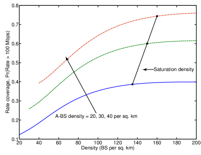
Figure 14: Rate distribution with variation in BS density but fixed A-BS density.

V Conclusion and future challenges

A baseline model and analytical framework is presented for characterizing the rate distribution in mmWave cellular networks. To the best of authors’ knowledge, the presented work is the first to integrate self-backhauling among BSs and co-existence with a conventional macrocellular network into the analysis of mmWave networks. We show that bandwidth plays minimal impact on the rate of power and noise-limited cell edge users, whereas increasing the BS density improves the corresponding rates drastically. This paper also further establishes the noise-limited nature of large bandwidth narrow beam-width mmWave networks. With self-backhauling, the rate saturates with increasing BS density for fixed A-BS density, where the corresponding saturation density is directly proportional to the A-BS density. The explicit characterization of the rate distribution as a function of key system parameters, which we provide, should help advance further the understanding of such networks and benchmark their performance.

The presented work can be extended in a number of directions. Offloading of indoor users, which may not even receive the signal from outdoor mmWave BSs, to more stable networks like $4$G or WiFi could be further investigated. Allowing multihop backhaul in sparser deployment of A-BSs could also be investigated in future work. The developed analytical framework also provides tools to analyze other network architectures like device-to-device (D2D) and ad hoc mmWave networks.

Appendix A

Proof:

We drop the subscript ‘a’ for access in this proof. The propagation process $\mathcal{N}\coloneqq L(X)=S(X)^{-1}\|X\|^{\alpha(X)}$ on for $X\in\Phi$, where $S\triangleq 10^{-(\chi+\beta)/10}$, has the intensity measure

$$\Lambda((0,t])=\int_{2}{\mathbb{P}}(L(X)<t)\mathrm{d}X=2\pi{\lambda}\int_{+}{\mathbb{P}}\left(\frac{r^{\alpha(r)}}{S(r)}<t\right)r\mathrm{d}r.$$

Denote a link to be of type $j$, where $j=l$ (LOS) and $j=n$ (NLOS) with probability $\mathrm{C}_{j,\mathrm{D}}$ for link length less than $\mathrm{D}$ and $\mathrm{C}_{j,\bar{\mathrm{D}}}$ otherwise. Note by construction $\mathrm{C}_{l,\mathrm{D}}+\mathrm{C}_{n,\mathrm{D}}=1$ and $\mathrm{C}_{l,\bar{\mathrm{D}}}+\mathrm{C}_{n,\bar{\mathrm{D}}}=1$. The intensity measure is then

$$\Lambda((0,t])=2\pi{\lambda}\sum_{j\in\{l,n\}}\mathrm{C}_{j,\mathrm{D}}\int_{+}{\mathbb{P}}\left(\frac{r^{\alpha_{j}}}{S_{j}}<t\right)\mathbbm{1}(r<\mathrm{D})r\mathrm{d}r$$

$$+\mathrm{C}_{j,\bar{\mathrm{D}}}\int_{+}{\mathbb{P}}\left(\frac{r^{\alpha_{j}}}{S_{j}}<t\right)\mathbbm{1}(r>\mathrm{D})r\mathrm{d}r$$

$$=2\pi{\lambda}\,\mathbb{E}\Bigg{[}\sum_{j\in\{l,n\}}(\mathrm{C}_{j,\mathrm{D}}-\mathrm{C}_{j,\bar{\mathrm{D}}})\frac{\mathrm{D}^{2}}{2}\mathbbm{1}(S_{j}>\mathrm{D}^{\alpha_{j}}/t)$$

$$+\mathrm{C}_{j,\mathrm{D}}\frac{(tS_{j})^{2/\alpha_{j}}}{2}\mathbbm{1}(S_{j}<\mathrm{D}^{\alpha_{j}}/t)+\mathrm{C}_{j,\bar{\mathrm{D}}}\frac{(tS_{j})^{2/\alpha_{j}}}{2}\mathbbm{1}(S_{j}>\mathrm{D}^{\alpha_{j}}/t)\Bigg{]}$$

$$={\lambda}\pi\sum_{j\in\{l,n\}}(\mathrm{C}_{j,\mathrm{D}}-\mathrm{C}_{j,\bar{\mathrm{D}}})\mathrm{D}^{2}\bar{F}_{S_{j}}(\mathrm{D}^{\alpha_{j}}/t)$$

$$+t^{2/{\alpha_{j}}}\left(\mathrm{C}_{j,\mathrm{D}}{\bar{\zeta}}_{S_{j},2/{\alpha_{j}}}(\mathrm{D}^{\alpha_{j}}/t)+\mathrm{C}_{j,\bar{\mathrm{D}}}{\underline{\zeta}}_{S_{j},2/\alpha_{j}}(\mathrm{D}^{\alpha_{j}}/t)\right),$$

where $\bar{F}_{S}$ denotes the CCDF of $S$, and ${\bar{\zeta}}_{S,n}(x),{\underline{\zeta}}_{S,n}(x)$ denote the truncated $n^{\text{th}}$ moment of $S$ given by $\bar{\zeta}_{S,n}(x)\triangleq\int_{0}^{x}s^{n}f_{S}(s)\mathrm{d}s$ and $\underline{\zeta}_{S,n}(x)\triangleq\int_{x}^{\infty}s^{n}f_{S}(s)\mathrm{d}s$. Since $S$ is a Lognormal random variable $\sim\mathrm{ln}\mathcal{N}(m,\sigma^{2})$, where $m=-0.1\beta\ln 10$ and $\sigma=0.1\xi\ln 10$. The intensity measure in Lemma 1 is then obtained by using

$$\bar{F}_{S}(x) =\mathrm{Q}\left(\frac{\ln x-m}{\sigma}\right),$$

$$\bar{\zeta}_{S,n}(x) ={\exp(\sigma^{2}n^{2}/2+mn)}\mathrm{Q}\left(\frac{\sigma^{2}n-\ln x+m}{\sigma}\right)$$

$$\underline{\zeta}_{S,n}(x) ={\exp(\sigma^{2}n^{2}/2+mn)}\mathrm{Q}\left(-\frac{\sigma^{2}n-\ln x+m}{\sigma}\right).$$

Now, since $\mathcal{N}$ is a PPP, the distribution of path loss to the tagged BS is then ${\mathbb{P}}(\inf_{X\in\Phi}L(X)>t)=\exp(-\Lambda((0,t]))$. ∎

Appendix B

Proof:

With fractional power control, a user transmits with a power $\mathrm{P}_{u}=\mathrm{P}_{0}L_{a}^{\epsilon}$ that partially compensates for path loss $L$, where $0\leq\epsilon\leq 1$ is the power control fraction (PCF) and $\mathrm{P}_{0}$ is the open loop power parameter. In this case, the uplink $\mathtt{SNR}$ CCDF is

$${\mathbb{P}}(\mathtt{SNR}_{u}>\tau) ={\mathbb{P}}\left(\frac{\mathrm{P}_{0}\mathrm{G_{max}}L_{a}(X^{*})^{\epsilon-1}}{\sigma^{2}_{N}}>\tau\right)$$

$$=1-\exp\left(-{\lambda}\mathrm{M}_{a}\left(\left(\frac{\mathrm{P}_{0}\mathrm{G_{max}}}{\tau\sigma^{2}_{N}}\right)^{1/(1-\epsilon)}\right)\right).$$

∎

Appendix C

Proof:

Having derived the intensity measure of $\mathcal{N}$ in Lemma 1, the distribution of $\mathtt{SINR}$ can be characterized on the same lines as [33]. The key steps are highlighted below for completeness.

$${\mathbb{P}}(\mathtt{SINR}>\tau)= {\mathbb{P}}\left(\frac{\mathrm{P}_{b}\mathrm{G_{max}}L(X^{*})^{-1}}{\sum_{X\in\Phi\setminus\{X^{*}\}}\mathrm{P}_{b}\psi_{X}L(X)^{-1}+\sigma^{2}_{N}}>\tau\right)$$

$$= {\mathbb{P}}\left(J+\frac{\sigma^{2}_{N}L(X^{*})}{\mathrm{P}_{b}\mathrm{G_{max}}}<\frac{1}{\tau}\right)$$

$$=\int_{l>0} {\mathbb{P}}\left(J+\frac{\sigma^{2}_{N}l}{\mathrm{P}_{b}\mathrm{G_{max}}}<\frac{1}{\tau}|L(X^{*})=l\right)f_{L(X^{*})}(l)\mathrm{d}l$$

where $J=\frac{L(X^{*})}{\mathrm{G_{max}}}\sum_{X\in\Phi\setminus\{X^{*}\}}\psi_{X}L(X)^{-1}$ and the distribution of $L(X^{*})$ is derived as

$$f_{L(X^{*})}(l)=-\frac{\mathrm{d}}{\mathrm{d}l}{\mathbb{P}}(L(X^{*})>l)={\lambda}\exp(-{\lambda}\mathrm{M}(l))\mathrm{M}^{{}^{\prime}}(l).$$ (8)

The conditional CDF required for the above computation is derived from the the conditional Laplace transform given below using the Euler’s characterization [34]

$$\mathcal{L}_{J,l}(z) ={\mathbb{E}\left[{\exp(-zJ)|L(X^{*})=l)}\right]}$$

$$=\exp\left(-{\mathbb{E}_{\psi}\left[{\int_{u>l}(1-\exp(-zl\psi/u))\Lambda(\mathrm{d}u)}\right]}\right),$$

where $\Lambda(\mathrm{d}u)$ is given by (4).

The inverse Laplace transform calculation required in the above derivation could get computationally intensive in certain cases and may render the analysis intractable. However, introducing Rayleigh small scale fading $H\sim\exp(1)$, on each link improves the tractability of the analysis as shown below. Coverage with fading is

$${\mathbb{P}}\left(\frac{\mathrm{P}_{b}\mathrm{G_{max}}H_{X^{*}}L(X^{*})^{-1}}{\sum_{X\in\Phi\setminus\{X^{*}\}}\mathrm{P}_{b}\psi_{X}H_{X}L(X)^{-1}+\sigma^{2}_{N}}>\tau\right)$$

$$= {\mathbb{E}\left[{\exp\left(-\frac{\tau\sigma^{2}_{N}}{\mathrm{P}_{b}\mathrm{G_{max}}}L(X^{*})-\tau L_{X^{*}}\sum_{X\in\Phi\setminus\{X^{*}\}}\frac{\psi_{X}}{\mathrm{G_{max}}}H_{X}L(X)^{-1}\right)}\right]}$$

$$\overset{(a)}{=} \int_{l>0}\exp\left(-\frac{\tau\sigma^{2}_{N}}{\mathrm{P}_{b}\mathrm{G_{max}}}l-{\lambda}{\mathbb{E}_{z}\left[{\int_{u>l}\frac{\mathrm{M}^{{}^{\prime}}(u)\mathrm{d}u}{u(zl)^{-1}+1}}\right]}\right)f_{L_{X^{*}}}(l)\mathrm{d}l$$

$$\overset{(b)}{=} {\lambda}\int_{l>0}\exp\left(-\frac{\tau\sigma^{2}_{N}}{\mathrm{P}_{b}\mathrm{G_{max}}}l-{\lambda}\mathrm{M}(l){\mathbb{E}_{\psi}\left[{\frac{1}{1+z}}\right]}\right)$$ (9)

$$\times\left(-{\lambda}{\mathbb{E}_{\psi}\left[{\int_{0}^{\frac{z}{z+1}}\mathrm{M}\left\{zl\left(\frac{1}{u}-1\right)\right\}\mathrm{d}u}\right]}\right)\mathrm{M}^{{}^{\prime}}(l)\mathrm{d}l,$$ (10)

where $z=\frac{\tau\psi}{\mathrm{G_{max}}}$, (a) follows using the Laplace functional of point process $\mathcal{N}$, (b) follows using integration by parts along with (8).

The above derivation assumed all BSs to be transmitting, but since user population is finite, certain BSs may not have a user to serve with probability $1-\mathsf{K}(\lambda_{u},{\lambda},0)$. This is incorporated in the analysis by modifying ${\lambda}\to{\lambda}(1-\mathsf{K}(\lambda_{u},{\lambda},0))$ in (a) above. ∎

Sarabjot Singh (S’09, M’15) received the B. Tech. in Electronics and Communication Engineering from Indian Institute of Technology Guwahati, India, in 2010 and the M.S.E and Ph.D. in Electrical Engineering from University of Texas at Austin. He is currently a Senior Researcher at Nokia Technologies, Berkeley, USA, where he is involved in the research and standardization of the next generation Wi-Fi systems. He has held industrial internships at Alcatel-Lucent Bell Labs in Crawford Hill, NJ; Intel Corp. in Santa Clara, CA; and Qualcomm Inc. in San Diego, CA. Dr. Singh was the recipient of the President of India Gold Medal in 2010 and the ICC Best Paper Award in 2013.

Mandar Kulkarni (S’13) received his B.Tech degree from the Indian Institute of Technology Guwahati in 2013 and was awarded the president of India gold medal for best academic performance. He is currently working towards his PhD in Electrical Engineering at the University of Texas at Austin. His research interests are broadly in the field of wireless communication, with current focus on modeling and analysis of cellular networks operating at millimeter wave frequencies. He has held internship positions at Nokia Networks, Arlington Heights, IL, U.S.A.; Technical University, Berlin, Germany and Indian Institute of Science, Bangalore, India in the years 2014, 2012 and 2011, respectively.

Amitabha Ghosh joined Motorola in 1990 after receiving his Ph.D in Electrical Engineering from Southern Methodist University, Dallas. Since joining Motorola he worked on multiple wireless technologies starting from IS-95, cdma-2000, 1xEV-DV/1XTREME, 1xEV-DO, UMTS, HSPA, 802.16e/WiMAX/802.16m, Enhanced EDGE and 3GPP LTE. Dr. Ghosh has 60 issued patents and numerous external and internal technical papers. Currently, he is Head, North America Radio Systems Research within the Technology and Innovation office of Nokia Networks. He is currently working on 3GPP LTE-Advanced and 5G technologies. His research interests are in the area of digital communications, signal processing and wireless communications. He is a Fellow of IEEE and co-author of the book titled “Essentials of LTE and LTE-A”.

Jeffrey Andrews (S’98, M’02, SM’06, F’13) received the B.S. in Engineering with High Distinction from Harvey Mudd College, and the M.S. and Ph.D. in Electrical Engineering from Stanford University. He is the Cullen Trust Endowed Professor ($\#$1) of ECE at the University of Texas at Austin, Editor-in-Chief of the IEEE Transactions on Wireless Communications, and Technical Program Co-Chair of IEEE Globecom 2014. He developed Code Division Multiple Access systems at Qualcomm from 1995-97, and has consulted for entities including Verizon, the WiMAX Forum, Intel, Microsoft, Apple, Samsung, Clearwire, Sprint, and NASA. He is a member of the Technical Advisory Boards of Accelera and Fastback Networks, and co-author of the books Fundamentals of WiMAX (Prentice-Hall, 2007) and Fundamentals of LTE (Prentice-Hall, 2010). Dr. Andrews received the National Science Foundation CAREER award in 2007 and has been co-author of ten best paper award recipients: ICC 2013, Globecom 2006 and 2009, Asilomar 2008, European Wireless 2014, the 2010 IEEE Communications Society Best Tutorial Paper Award, the 2011 IEEE Heinrich Hertz Prize, the 2014 EURASIP Best Paper Award, the 2014 IEEE Stephen O. Rice Prize, and the 2014 IEEE Leonard G. Abraham Prize. He is an IEEE Fellow and an elected member of the Board of Governors of the IEEE Information Theory Society.

References

- [1] S. Singh, M. N. Kulkarni, and J. G. Andrews, “A tractable model for rate in noise limited mmwave cellular networks,” in Asilomar Conf. on Signals, Systems and Computers, Nov. 2014.
- [2] Cisco, “Cisco visual networking index: Global mobile data traffic forecast update, 2013-2018.” Whitepaper, available at: http://goo.gl/SwuEIc.
- [3] F. Boccardi, R. W. Heath, A. Lozano, T. L. Marzetta, and P. Popovski, “Five disruptive technology directions for 5G,” IEEE Commun. Mag., vol. 52, pp. 74–80, Feb. 2014.
- [4] T. Rappaport et al., “Millimeter wave mobile communications for 5G cellular: It will work!,” IEEE Access, vol. 1, pp. 335–349, May 2013.
- [5] J. G. Andrews et al., “What will 5G be?,” IEEE J. Sel. Areas Commun., vol. 32, pp. 1065–1082, June 2014.
- [6] T. Baykas et al., “IEEE 802.15.3c: The first IEEE wireless standard for data rates over 1 Gb/s,” IEEE Commun. Mag., vol. 49, pp. 114–121, July 2011.
- [7] R. C. Daniels, J. N. Murdock, T. S. Rappaport, and R. W. Heath, “60 GHz wireless: Up close and personal,” IEEE Microw. Mag., vol. 11, pp. 44–50, Dec. 2010.
- [8] Z. Pi and F. Khan, “An introduction to millimeter-wave mobile broadband systems,” IEEE Commun. Mag., vol. 49, pp. 101–107, June 2011.
- [9] W. Roh et al., “Millimeter-wave beamforming as an enabling technology for 5G cellular communications: Theoretical feasibility and prototype results,” IEEE Commun. Mag., vol. 52, pp. 106–113, Feb. 2014.
- [10] T. Rappaport et al., “Broadband millimeter-wave propagation measurements and models using adaptive-beam antennas for outdoor urban cellular communications,” IEEE Trans. Antennas Propag., vol. 61, pp. 1850–1859, Apr. 2013.
- [11] S. Rangan, T. Rappaport, and E. Erkip, “Millimeter-wave cellular wireless networks: Potentials and challenges,” Proceedings of the IEEE, vol. 102, pp. 366–385, Mar. 2014.
- [12] M. R. Akdeniz et al., “Millimeter wave channel modeling and cellular capacity evaluation,” IEEE J. Sel. Areas Commun., vol. 32, pp. 1164–1179, June 2014.
- [13] S. Larew, T. Thomas, and A. Ghosh, “Air interface design and ray tracing study for 5G millimeter wave communications,” IEEE Globecom B4G Workshop, pp. 117–122, Dec. 2013.
- [14] A. Ghosh et al., “Millimeter wave enhanced local area systems: A high data rate approach for future wireless networks,” IEEE J. Sel. Areas Commun., vol. 32, pp. 1152–1163, June 2014.
- [15] M. Abouelseoud and G. Charlton, “System level performance of millimeter-wave access link for outdoor coverage,” in IEEE WCNC, pp. 4146–4151, Apr. 2013.
- [16] M. N. Kulkarni, S. Singh, and J. G. Andrews, “Coverage and rate trends in dense urban mmWave cellular networks,” in IEEE Global Commun. Conf. (GLOBECOM), Dec. 2014.
- [17] S. Singh, R. Mudumbai, and U. Madhow, “Interference analysis for highly directional 60 GHz mesh networks: The case for rethinking medium access control,” IEEE/ACM Trans. Netw., vol. 19, pp. 1513–1527, Oct. 2011.
- [18] Interdigital, “Small cell millimeter wave mesh backhaul,” Feb. 2013. Whitepaper, available at: http://goo.gl/Dl2Z6V.
- [19] R. Taori and A. Sridharan, “In-band, point to multi-point, mm-Wave backhaul for 5G networks,” in IEEE Intl. Workshop on 5G Tech., ICC, pp. 96–101, June 2014.
- [20] J. S. Kim, J. S. Shin, S.-M. Oh, A.-S. Park, and M. Y. Chung, “System coverage and capacity analysis on millimeter-wave band for 5G mobile communication systems with massive antenna structure,” Intl. Journal of Antennas and Propagation, vol. 2014, July 2014.
- [21] M. Coldrey, J.-E. Berg, L. Manholm, C. Larsson, and J. Hansryd, “Non-line-of-sight small cell backhauling using microwave technology,” IEEE Commun. Mag., vol. 51, pp. 78–84, Sept. 2013.
- [22] S. W. Peters, A. Y. Panah, K. T. Truong, and R. W. Heath, “Relay architectures for 3GPP LTE-advanced,” EURASIP Journal on Wireless Communications and Networking, 2009.
- [23] S. Akoum, O. El Ayach, and R. Heath, “Coverage and capacity in mmWave cellular systems,” in Asilomar Conf. on Signals, Systems and Computers, pp. 688–692, Nov. 2012.
- [24] T. Bai and R. W. Heath, “Coverage and rate analysis for millimeter wave cellular networks,” IEEE Trans. Wireless Commun., vol. 14, pp. 1100–1114, Feb. 2015.
- [25] T. Bai and R. W. Heath, “Coverage analysis for millimeter wave cellular networks with blockage effects,” in IEEE Global Conf. on Signal and Info. Processing (GlobalSIP), pp. 727–730, Dec. 2013.
- [26] T. Bai, R. Vaze, and R. W. Heath, “Analysis of blockage effects on urban cellular networks,” IEEE Trans. Wireless Commun., vol. 13, pp. 5070–5083, Sept. 2014.
- [27] S. Singh, H. S. Dhillon, and J. G. Andrews, “Offloading in heterogeneous networks: Modeling, analysis, and design insights,” IEEE Trans. Wireless Commun., vol. 12, pp. 2484–2497, May 2013.
- [28] J. G. Andrews, S. Singh, Q. Ye, X. Lin, and H. S. Dhillon, “An overview of load balancing in HetNets: Old myths and open problems,” IEEE Wireless Commun. Mag., vol. 21, pp. 18–25, Apr. 2014.
- [29] A. Guo and M. Haenggi, “Asymptotic deployment gain: A simple approach to characterize the distribution in general cellular networks,” IEEE Trans. Commun., vol. 63, pp. 962–976, Mar. 2015.
- [30] S. Yi, Y. Pei, and S. Kalyanaraman, “On the capacity improvement of ad hoc wireless networks using directional antennas,” in Intl. Symp. on Mobile Ad Hoc Networking and Computing, MobiHoc, pp. 108–116, 2003.
- [31] J. Wildman, P. H. J. Nardelli, M. Latva-aho, and S. Weber, “On the joint impact of beamwidth and orientation error on throughput in wireless directional Poisson networks,” IEEE Trans. Wireless Commun., vol. 13, pp. 7072–7085, Dec. 2014.
- [32] Q. C. Li, H. Niu, G. Wu, and R. Q. Hu, “Anchor-booster based heterogeneous networks with mmWave capable booster cells,” IEEE Globecom B4G Workshop, pp. 93–98, Dec. 2013.
- [33] B. Blaszczyszyn, M. K. Karray, and H.-P. Keeler, “Using Poisson processes to model lattice cellular networks,” in Proc. IEEE Intl. Conf. on Comp. Comm. (INFOCOM), pp. 773–781, Apr. 2013.
- [34] J. Abate and W. Whitt, “Numerical inversion of Laplace transforms of probability distributions,” ORSA Journal on Computing, vol. 7, no. 1, pp. 36–43, 1995.
- [35] S. Singh, “Matlab code for numerical computation of total power to noise ratio in mmW networks.” [Online]. Available : http://goo.gl/Au30J4.
- [36] S. Singh, F. Baccelli, and J. G. Andrews, “On association cells in random heterogeneous networks,” IEEE Wireless Commun. Lett., vol. 3, pp. 70–73, Feb. 2014.
- [37] S. M. Yu and S.-L. Kim, “Downlink capacity and base station density in cellular networks,” in Intl. Symp. on Modeling Optimization in Mobile Ad Hoc Wireless Networks (WiOpt), pp. 119–124, May 2013.
- [38] J. G. Andrews, F. Baccelli, and R. K. Ganti, “A tractable approach to coverage and rate in cellular networks,” IEEE Trans. Commun., vol. 59, pp. 3122–3134, Nov. 2011.