Spreading of intolerance under economic stress: results from a model with reputation.

Abstract

When a population is engaged in successive prisoner’s dilemmas, indirect reciprocity through reputation fosters cooperation through the emergence of moral and action rules. A simplified model has recently been proposed where individuals choose between helping or not others, and are judged good or bad for it by the rest of the population. The reputation so acquired will condition future actions. In this model, eight strategies (referred to as ‘leading eight’) enforce a high level of cooperation, generate high payoffs and are therefore resistant to invasions by other strategies. Here we show that, by assigning each individual one out of two labels that peers can distinguish (e.g., political ideas, religion, skin colour…) and allowing moral and action rules to depend on the label, intolerant behaviours can emerge within minorities under sufficient economic stress. We analyse the sets of conditions where this can happen and also discuss the circumstances under which tolerance can be restored. Our results agree with empirical observations that correlate intolerance and economic stress, and predict a correlation between the degree of tolerance of a population and its composition and ethical stance.

I Introduction

Different kinds of discriminatory behaviour based on membership to different groups—identified, for example, by visible tags Hamilton (1964)—has been reported both in human Sumner (1906); LeVine and Campbell (1972); Hirschfeld (1996); Bernhard et al. (2006) and in animal societies Haig (1996); Keller and Ross (1998); Queller et al. (2003); Summers and Crespi (2005); Sinervo et al. (2006). They can be broadly classified into two main types: in-group favoritism and out-group hostility Ray and Lovejoy (1986); Struch and Schwartz (1989); Cashdan (2001). Recent studies of in-group and out-group cooperation show that in-group favouritism can emerge in the framework of indirect reciprocity Masuda (2012); Nakamura and Masuda (2012); Oishi et al. (2012).

The concept of indirect reciprocity Sugden (1986); Alexander (1987) has been introduced to explain the emergence of cooperation in society, where many interactions between the same individuals have low chances to be repeated. Contrary to direct reciprocity Trivers (1971), indirect reciprocity implies that individuals receive the consequences of their actions, not directly from their opponents, but indirectly through society. Indirect reciprocity—and its related reputation concept—has proven to be an important mechanism for the emergence and sustainment of cooperation in small-scale human Dufwenberg et al. (2001); Milinski et al. (2002); Panchanathan and Boyd (2004); Semmann et al. (2004); Suzuki and Akiyama (2007) and non-human Bshary and Gutter (2006) societies. It also plays an important role in communication networks Bolton et al. (2005); Keser (2002). In these reputation-based models, individuals have an opinion about every interaction they witness and assign a reputation to the individuals involved accordingly Nowak and Sigmund (1998); Ohtsuki and Iwasa (2004); Brandt and Sigmund (2004); Nowak and Sigmund (2005); Milinski et al. (2002). The nature of their future interactions with those individuals will be determined by the reputation they have assigned to them.

In a stylised model of indirect reciprocity Ohtsuki and Iwasa Ohtsuki and Iwasa (2004) and Brandt and Sigmund Brandt and Sigmund (2004) classified the strategies involved in these games attending to action and assessment modules. The action module prescribes what to do—whether cooperate or not—given the reputations of the individuals involved. The assessment module assigns reputation to the interacting individuals according to a moral code. To do it three elements can be judged: the nature of the interaction, the reputation of the recipient, and the reputation of the donor. Strategies are thus classified as first, second, or third order depending on whether the first, the first and the second, or all the three elements are taken into account to assign a reputation to the donor. Ohtsuki and Iwasa Ohtsuki and Iwasa (2004) studied the evolutionarily stability of third order strategies which share the same moral assessment module, and later Martinez-Vaquero and Cuesta Martinez-Vaquero and Cuesta (2013) extended the study confronting strategies with different moral codes. Among the evolutionary stable strategies (ESS) found, there are eight strategies—the so-called Leading Eight—that are considerably more efficient (get very high payoff) and coherent (in terms of consistency between their moral and action modules) than the rest of them. All these strategies foster cooperation through indirect reciprocity.

This simple model of indirect reciprocity can be readily extended to study the emergence of discriminatory behaviours by introducing different groups of individuals identified by external signs (these may include physical or cultural traits). Our goal in this work is to analyse under which conditions an intolerant strategy (understood as out-group hostility) can invade a tolerant population that follows one of the Leading Eight strategies. Whenever intolerance spreads, we are also interested in whether tolerance can be restored by introducing some kind of external incentives. Our hope is that this study sheds some light into the causes for the emergence of intolerance in societies and the mechanisms to alleviate this social burden.

The paper is structured as follows. In section II we introduce the model, which is mathematically implemented in section III. Our results are shown in section IV and discussed in section V.

II Model

Our model is an extension of that used in a previous work Martinez-Vaquero and Cuesta (2013)—itself a modification of the indirect reciprocity model based on reputation introduced by Brandt and Sigmund Brandt and Sigmund (2004) and later investigated by Ohtsuki and Iwasa Ohtsuki and Iwasa (2004, 2006).

We consider an infinite, well-mixed population, where every individual is aware of every action performed and produces a moral judgment—which leads to a reputation assignment—on it. Each time step a pair of individuals is randomly drawn—with equal probability—from the population. One of them plays as donor and the other one as recipient. The donor can decide to pay a cost $c>0$ to help (C) the recipient or not (D). Any helped recipient gains a payoff $b>c$; otherwise there is no payoff whatsoever.

This action is observed by every individual in the population (including themselves). Thus everyone makes a private judgment of the donor for this action. The observer’s moral assessment will decide the reputation—good (G) or bad (B)—she assigns to the donor. Accordingly, everybody has a private opinion of every other individual—even of herself.

By repeating this process the population eventually reaches a steady state. The average payoff of this repeated game is then computed for every individual. By assuming a very large population we effectively neglect direct reciprocity—the probability that two individuals meet again is very small.

Strategies are defined by two modules: the action rules, which tells the donor how to interact with the recipient, and the moral rules, which prescribe a reputation for the donor of every witnessed action. As in our previous paper Martinez-Vaquero and Cuesta (2013), we will consider third order strategies.

The action rules determine what the donor must do (either help or refuse to help) given the reputation of both players. Specifically, $a_{\alpha\beta}=1$ (C) if a strategist with reputation $\alpha$ helps an individual with reputation $\beta$ and $0$ (D) otherwise.

The moral assessments tell the individual if the action just witnessed should be judged good or bad, hence revising the donor’s reputation. Specifically, $m_{\alpha\beta}(a)=1$ (G) if the observer assigns good reputation to a donor she previously judged $\alpha$, who performs an action $a$ on an recipient she previously judged $\beta$, and is $0$ (B) otherwise.

Thus each strategy is defined by 12 numbers: 4 for the action module and 8 for the moral module. This amounts to 4096 different strategies in total.

Besides, we will assume that players sometimes make errors when trying to help another individual Leimar and Hammerstein (2001); Ohtsuki and Iwasa (2004); Panchanathan and Boyd (2003); Fishman (2003); Lotem et al. (1999). Thus, with a probability $\epsilon$ a donor defects regardless of her action rules and with $1-\epsilon$ she performs the action she planned to. One possible source of this error—which will be important in interpreting the results of this work—is scarcity of resources. Despite her willingness to help, an individual may fail to do it because she cannot afford the cost $c$. Errors due to misjudgements are excluded (see Martinez-Vaquero and Cuesta (2013) for a justification).

Discrimination requires at least two different subpopulations that can be clearly identified by everybody. Thus we divide our population into two classes, A and B. The fraction of A individuals will be denoted $y$. A tolerant player will act disregarding the individuals’ class when deciding her action or judgement. An intolerant individual acts and judges like a tolerant one with the following exceptions:

1. Individuals of the other class are never helped.

2. Donors of the other class are judged bad under any circumstance.

3. Individuals of her own class who do not help individuals of the other class are always judged good.

4. Individuals of her own class who do help individuals of the other class are always judged bad.

III Implementation

Our goal is to determine, with the assumptions of the model, under which conditions a small population of intolerant (tolerant) mutants $M$ can invade a tolerant (intolerant) resident population $R$ made of A-type and B-type individuals in fractions $y$ and $1-y$ respectively. This fraction $y$ will be kept constant and is therefore a parameter of the model. We will only consider scenarios where all individuals of the same class in $R$ show the same kind of behavior—either tolerant or intolerant—toward the other class. Likewise, we will limit ourselves to determine when the resident population can resist the invasion of mutants. Determining the final composition of the population if the invasion succeeds is a more complex problem that we will tackle in this paper.

Without loss of generality, in the following calculations mutants will be assumed to belong to class A. Likewise, we will only need to consider whether A-residents imitate the mutant or not. If a B-resident imitates the A-mutant (its tolerant or intolerant character) this can be treated as an invasion of B-residents by a B-mutant separately—the reason being that mutants are present in so small a fraction that the probability that two mutants interact is negligible.

Accordingly the different invasion scenarios will be denoted $t_{M}|t_{\text{A}}t_{\text{B}}$, where $t_{X}$ can be either T (tolerant individuals) or I (intolerant individuals), $M$ denotes A-type mutants, and A and B the two subpopulations. The four possible scenarios are:

I$|$TT

intolerant A-mutants try to invade a tolerant population;

T$|$IT

tolerant A-mutants try to invade a population made of intolerant A-residents and tolerant B-residents;

I$|$TI

intolerant A-mutants try to invade a population made of tolerant A-residents and intolerant B-residents;

T$|$II

tolerant A-mutants try to invade an intolerant population.

The condition for A-residents to resist the invasion of A-mutants is $W(A|R)>W(M|R)$, where $W(A|R)$ and $W(M|R)$ are the average payoffs received by A-type residents and by mutants, respectively. They can be obtained as

$$\begin{split}W(A|R)&=b\ \Theta_{R,A}-c\ \Theta_{A,R},\\ W(M|R)&=b\ \Theta_{R,M}-c\ \Theta_{M,R},\\ \Theta_{R,A}&=y\ \theta_{A,A}+(1-y)\ \theta_{B,A},\\ \Theta_{A,R}&=y\ \theta_{A,A}+(1-y)\ \theta_{A,B},\\ \Theta_{R,M}&=y\ \theta_{A,M}+(1-y)\ \theta_{B,M},\\ \Theta_{M,R}&=y\ \theta_{M,A}+(1-y)\ \theta_{M,B},\end{split}$$ (1)

where $\theta_{i,j}$ is the probability that an $i$-strategist helps a $j$-strategist. If $i$-strategists are intolerant and $j$-strategists belong to a different class $\theta_{i,j}=0$; otherwise these probabilities can be obtained as

$$\theta_{i,j}=(1-\epsilon)\sum_{\alpha\beta}\chi_{\alpha}(g_{i}^{i})\chi_{\beta}(g_{j}^{i})a_{\alpha\beta},$$ (2)

where $g_{i}^{j}$ is the fraction of $i$-strategists that are considered good by the $j$-strategists. We have introduced the auxiliary function

$$\chi_{\gamma}(x)=\gamma x+(1-\gamma)(1-x).$$ (3)

Thus if $x$ represent the fraction of good individuals, then $\chi_{1}(x)=x$ and $\chi_{0}(x)=1-x$ are the fraction of ‘good’ and ‘bad’ individuals, respectively.

In order to calculate the fractions $g_{i}^{j}$ we first need to compute the fractions $x_{i}^{\Lambda_{A}\Lambda_{B}\Lambda_{M}}$ of $i$-individuals with reputations $\Lambda_{A}$, $\Lambda_{B}$, and $\Lambda_{M}$ according to A-residents, B-residents, and mutants, respectively. Here $\Lambda_{i}$ can be G (for good reputation), B (for bad reputation), or * (for any reputation, G or B). For instance, $x_{i}^{G*B}$ represents the fraction of $i$-type individuals who are considered good by A-residents and bad by mutants, regardless of B-residents’ opinion. Hence $x_{i}^{G*B}=\sum_{\Lambda_{B}}x_{i}^{G\Lambda_{B}B}$. Thus

$$g_{i}^{A}=x_{i}^{G**},\qquad g_{i}^{B}=x_{i}^{*G*},\qquad g_{i}^{M}=x_{i}^{**G}.$$ (4)

It turns out that not all $x_{i}^{\Lambda_{A}\Lambda_{B}\Lambda_{M}}$ are necessary to compute $g_{i}^{j}$ (see Appendix for details). In general, all we need is to obtain $x_{A}^{\Lambda_{A}*\Lambda_{M}}$, $x_{M}^{\Lambda_{A}*\Lambda_{M}}$, and for some scenarios also $x_{B}^{\Lambda_{A}*\Lambda_{M}}$ or $x_{B}^{*\Lambda_{B}\Lambda_{M}}$. Since we are considering an infinite population, self-interactions are negligible. Under the assumption that the rate of mutants is very low, donors will only interact with residents and therefore the dynamics of these fractions will be given by

$$\frac{dx_{A}^{\Lambda_{A}*\Lambda_{M}}}{dt} =y\ T_{A,A}^{\Lambda_{A}\Lambda_{M}}+(1-y)\ F_{A,B}^{\Lambda_{A}\Lambda_{M}}-x_{A}^{\Lambda_{A}*\Lambda_{M}},$$ (5)

$$\frac{dx_{B}^{\Lambda_{A}\Lambda_{B}*}}{dt} =(1-y)\ T_{B,B}^{\Lambda_{A}\Lambda_{B}}+y\ F_{B,A}^{\Lambda_{A}\Lambda_{B}}-x_{B}^{\Lambda_{A}*\Lambda_{B}},$$ (6)

$$\frac{dx_{B}^{*\Lambda_{B}\Lambda_{M}}}{dt} =(1-y)\ T_{B,B}^{\Lambda_{B}\Lambda_{M}}+y\ F_{B,A}^{\Lambda_{B}\Lambda_{M}}-x_{B}^{*\Lambda_{B}\Lambda_{M}},$$ (7)

$$\frac{dx_{M}^{\Lambda_{A}*\Lambda_{M}}}{dt} =y\ T_{M,A}^{\Lambda_{A}\Lambda_{M}}+(1-y)\ F_{M,B}^{\Lambda_{A}\Lambda_{M}}-x_{M}^{\Lambda_{A}*\Lambda_{M}},$$ (8)

where the interactions with recipients of the same and of the opposite class have been split into $T_{i,j}^{\Lambda_{l}\Lambda_{m}}$ and $F_{i,j}^{\Lambda_{l}\Lambda_{m}}$, respectively. Fractions $F_{i,j}^{\Lambda_{l}\Lambda_{m}}$ depend on the scenario we are considering whereas $T_{i,j}^{\Lambda_{l}\Lambda_{m}}$ are common for all of them and can be obtained as

$$T_{i,A}^{\Lambda_{A}\Lambda_{M}}= \sum_{\alpha_{A}\alpha_{M}\beta_{A}\beta_{M}}x_{i}^{\alpha_{A}*\alpha_{M}}x_{A}^{\beta_{A}*\beta_{M}}$$

$$\times R^{\Lambda_{A}\Lambda_{M}}(\alpha_{A}\beta_{A},\alpha_{M}\beta_{M}|\alpha_{i}\beta_{i})$$ (9)

$$T_{B,B}^{\Lambda_{A}\Lambda_{B}}= \sum_{\alpha_{A}\alpha_{B}\beta_{A}\beta_{B}}x_{B}^{\alpha_{A}\alpha_{B}*}x_{B}^{\beta_{A}\beta_{B}*}$$

$$\times R^{\Lambda_{A}\Lambda_{B}}(\alpha_{A}\beta_{A},\alpha_{B}\beta_{B}|\alpha_{B}\beta_{B})$$ (10)

$$T_{B,B}^{\Lambda_{B}\Lambda_{M}}= \sum_{\alpha_{B}\alpha_{M}\beta_{B}\beta_{M}}x_{B}^{*\alpha_{B}\alpha_{B}}x_{B}^{*\beta_{B}\beta_{M}}$$

$$\times R^{\Lambda_{B}\Lambda_{M}}(\alpha_{B}\beta_{B},\alpha_{M}\beta_{M}|\alpha_{B}\beta_{B})$$ (11)

where $R^{\Lambda_{l}\Lambda_{m}}(\alpha_{l}\beta_{l},\alpha_{m}\beta_{m}|\alpha_{i}\beta_{i})$ is the probability that an $i$-type donor with reputation $(\alpha_{l},\alpha_{m})$ acting on a recipient with reputation $(\beta_{l},\beta_{m})$, is assigned a reputation $(\Lambda_{l},\Lambda_{m})$. Reputations are as given by $l$-individuals and $m$-individuals respectively. This probability is obtained as

$$\begin{split}R^{\Lambda_{l}\Lambda_{m}}&(\alpha_{l}\beta_{l},\alpha_{m}\beta_{m}|\alpha_{i}\beta_{i})=\\ &=(1-\epsilon)\,\delta\big{(}\Lambda_{l},m_{\alpha_{l}\beta_{l}}(a_{\alpha_{i}\beta_{i}})\big{)}\delta\big{(}\Lambda_{m},m_{\alpha_{m}\beta_{m}}(a_{\alpha_{i}\beta_{i}})\big{)}\\ &+\,\epsilon\,\delta\big{(}\Lambda_{l},m_{\alpha_{l}\beta_{l}}(D)\big{)}\delta\big{(}\Lambda_{m},m_{\alpha_{m}\beta_{m}}(D)\big{)}.\end{split}$$ (12)

In general, Eqs. (5)–(8) need to be solved numerically. Nevertheless, for the different scenarios that we will consider, some simplifications can be made. The details are deserved to the Appendix.

IV Results

	$m_{GG}(C)$	$m_{GG}(D)$	$m_{GB}(C)$	$m_{GB}(D)$	$m_{BG}(C)$	$m_{BG}(D)$	$m_{BB}(C)$	$m_{BB}(D)$	$a_{GG}$	$a_{GB}$	$a_{BG}$	$a_{BB}$
Ia	G	B	G	G	G	B	G	B	C	D	C	C
Ib	G	B	B	G	G	B	G	B	C	D	C	C
IIa	G	B	G	G	G	B	G	G	C	D	C	D
IIb	G	B	G	G	G	B	B	G	C	D	C	D
IIc	G	B	B	G	G	B	G	G	C	D	C	D
IId	G	B	B	G	G	B	B	G	C	D	C	D
IIIa	G	B	G	G	G	B	B	B	C	D	C	D
IIIb	G	B	B	G	G	B	B	B	C	D	C	D

Table 1: Leading eight strategies. The first eight columns describe the moral assessment; the last four, the action rules. Strategies are classified into three groups (I, II, and III; see text).

We focus our analysis on the leading eight strategies introduced by Ohtsuki and Iwasa Ohtsuki and Iwasa (2004). In a previous paper Martinez-Vaquero and Cuesta (2013) we proved that, for reasonable values of benefit-to-cost and error rates, these eight strategies are evolutionarily stable against the invasion of any other strategy. On the other hand, Ohtsuki and Iwasa Ohtsuki and Iwasa (2004) classified the leading eight in three groups (Table 1), according to their stability against invasions by fully defective action rules (AllD). Neglecting errors in the moral assessment, Groups I and II can be invaded by AllD provided

$$\frac{b}{c}<1+\epsilon+\epsilon^{2}+\dots=\frac{1}{1-\epsilon},$$ (13)

in other words, if the error in the action $\epsilon>(b-c)/b$. Invading Group III requires $b<c$ though.

Therefore, for a given $b>c$, if $\epsilon$ is sufficiently large, any Group I or Group II strategy can be invaded by defectors, whereas Group III strategies always resist invasions. As we will show below, these are the same conditions under which intolerance can spread, but intolerant strategies obtain a higher payoff than AllD because they are indistinguishable from the strategy used by residents of their same group. Accordingly, when two distinguishable groups coexist in a population, intolerant strategies are preferred over AllD.

Figure 1: (Color online.) Values for $\epsilon$ and $y$ indicating the different regions where invasions $I|TT$, $T|IT$ and $IT|I$ are successful for strategy Ia. Above the horizontal line, also AllD can invade a tolerant population.

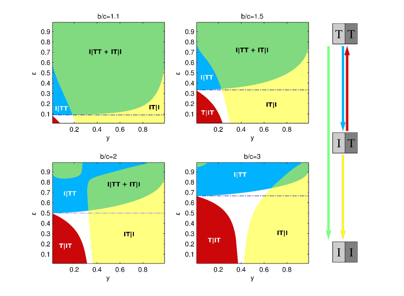
Figure 2: (Color online.) Same as Fig. 1 but for strategy Ib.

Figure 3: (Color online.) Same as Fig. 1 but for strategy IIa.

Figure 4: (Color online.) Same as Fig. 1 but for strategy IIb.

Figure 5: (Color online.) Same as Fig. 1 but for strategy IIc.

Figure 6: (Color online.) Same as Fig. 1 but for strategy IId.

Figure 7: (Color online.) Same as Fig. 1 but for strategy IIIa, with the new invasion scenario $II|T$.

Figure 8: (Color online.) Same as Fig. 7 but for strategy IIIb.

In what follows we will consider the different invasion scenarios for which there exists a parameter region where invasion occurs. These regions are determined numerically, and represented in Figs. 1–8 as colored areas in a $\epsilon$–$y$ plane, where $y$ represents the fraction of A-residents in the community. For the sake of clarity of the representations, we will sometimes assume that the invader is of type A, and sometimes of type B. Consistent with the previous section, we will denote $t_{M}|t_{A}t_{B}$—$t_{X}=\,$T,I being the tolerant/intolerant character of type X individuals—whenever the mutant is of type A, and $t_{A}t_{B}|t_{M}$ whenever the mutant is of type B. (Notice, however, that $y$ will always represent the fraction of A-residents, which will coincide with the type of mutants in the former case, but not in the latter.) Changing the type of mutant will make analyzing successive invasions $I|TT$ and $IT|I$ —which would turn a fully tolerant population into a fully intolerant one— much easier.

In all invasion scenarios that we will consider, we will just determine the stability of the resident population against invasion by mutants, but not the final equilibrium (hence we do not determine whether there is a turnover of the invaded population or a final coexistence is reached). Figures 1–6 correspond to Group I and Group II strategies, whereas Figs. 7–8 correspond to Group III strategies.

The different scenarios are as follows: $I|TT$, $T|IT$, $IT|I$, and $T|II$. Overlaps of these regions are colored by a mixed color.

First of all, Figures 1–6 show that tolerant communities that follow Group I and Group II strategies can be invaded by intolerant individuals ($I|TT$) if $\epsilon$ is sufficiently high and/or $b/c$ sufficiently low. Minorities are more prone to undergo such a spread of intolerance. Second, if one of the two resident types is intolerant and the other one is tolerant, intolerant residents can be invaded by tolerant mutants ($T|IT$) provided they are a minority (in all cases that we have analysed $y<0.5$). However, this $T|IT$ region never overlaps with the $I|TT$ one, so after a spread of intolerance the “economic conditions” must change for tolerance to be restored. Third, if in a community with tolerant and intolerant residents the latter are the majority, then this strategy can spread also among the tolerant residents ($IT|I$), thus dividing the community into two separate groups that dislike and never help each other. And finally, a fully intolerant community resists invasion by tolerant individuals for any combination of parameters. Hence, there is no way to restore tolerance in a fully intolerant community by tuning the parameters of the model (but see Section IV.1).

If we associate low $b/c$ ratios and high $\epsilon$ with strait conditions, the interpretation emerging from these results is that economic stress favors the spread of intolerance within minorities. Once it has invaded a group, tolerance cannot be restored unless the economic conditions improve. And if intolerance has eventually split the community, not even that can restore tolerance again.

Group III strategies are quite different (Figs. 7–8). A tolerant population following any of these strategies always resists the invasions of intolerant mutants regardless of the parameter setting (i.e., invasion $I|TT$ never happens). Furthermore, if one type is tolerant and the other one intolerant in the resident population, tolerant mutants can invade the intolerant residents ($T|IT$). Intolerant mutants can also invade the tolerant residents ($IT|I$), but this occurs in a much narrower region of the diagram compared to what happens for Group I and Group II strategies. As a matter of fact, intolerant mutants only succeed if they try to invade a minority of tolerant residents when the rest of the community is intolerant. Furthermore if we start from a society where both subpopulations are intolerant, tolerant mutants have a chance to invade the minority and spread their strategy ($II|T$) —and perhaps eventually turn the community into tolerant individuals in the brown region, overlap between $II|T$ and $T|IT$ invasion regions. Overall, Group III strategies prove more stable against intolerance.

IV.1 Incentives to restore tolerance

Figure 9: (Color online.) Conditions of $\epsilon$ and $y$ under which the invasions $T^{\prime}|II$, $I|T^{\prime}I$ and $T^{\prime}I|T$ are successful for Ib (left) and IId (right) strategies. Incentivated cost $c^{\prime}=0$.

As shown in the previous section, if a tolerant community—or one of the two subpopulations within it—following a Group I or a Group II strategy eventually becomes intolerant, there is no way to restore tolerance again by spreading it among the intolerant individuals. The only way to achieve this is by “improving the economic conditions” (i.e., decreasing $\epsilon$ and/or increasing $b/c$). An alternative way to generate the same effect could be introducing an exogenous incentive. We have implemented one such policy through a reduction of the cost of helping others. In other words, we assume the presence of a super-agent who partly subsidises the cost of helping individuals of a subpopulation. This is done by lowering the cost of helping $B$-strategists. By assuming this cost $c^{\prime}<c$, Eqs. (1) turn into

$$\begin{split}W^{\prime}(A|R)&=b\ \Theta_{R,A}-\Theta^{\prime}_{A,R},\\ W^{\prime}(M|R)&=b\ \Theta_{R,M}-\Theta^{\prime}_{M,R},\end{split}$$ (14)

where

$$\begin{split}\Theta^{\prime}_{A,R}&=c\ \theta_{A,A}+c^{\prime}\ \theta_{A,B},\\ \Theta^{\prime}_{M,R}&=c\ \theta_{M,A}+c^{\prime}\ \theta_{M,B}.\end{split}$$ (15)

The new scenarios where individuals of a class are given incentives to help the other class are $I|T^{\prime}T$, $T^{\prime}|IT$, $I|T^{\prime}I$, and $T^{\prime}|II$, where primes mark individuals who pay the lower cost $c^{\prime}$ for helping the opposite class. Equations (14) must be used for these individuals, whereas non-primed individuals follow Eqs. (1), as usual. Intolerant individuals are never marked since they never never help the opposite class anyway.

From now on we focus only in Groups I and Group II strategies because tolerant populations following Group III strategies are intolerance-proof. The most effective incentive is reached for $c^{\prime}=0$ (i.e., helping the opposite class is free). Since strategies belonging to the same group have a very similar behaviour, we show only one example for each group in Figs. 9-10.

Starting from a fully intolerant population, we represent in Fig. 9 the region where incentives are able to promote tolerance in one of the subpopulation ($T^{\prime}|II$). Wherever this invasion succeeds, the situation cannot be reverted, i.e., invasions $I|T^{\prime}I$ never occur for the same parameter values ($I|T^{\prime}I$ and regions $T^{\prime}|II$ do not overlap). But on the other hand, intolerant residents in a $T^{\prime}I$ population cannot be invaded by tolerant mutants ($T^{\prime}I|T$) for the same parameter values (again, $T^{\prime}I|T$ and $T^{\prime}|II$ regions do not overlap). In other words, if incentives promote tolerance in one subpopulation of fully intolerant individuals, the other subpopulation will still resist invasions by tolerant mutants. Incentives are thus not enough to make a fully tolerant community.

On the other hand, Figure 10 shows that the region of $T^{\prime}I|T^{\prime}$ invasions does overlap with the region of $T^{\prime}|II$ invasions. Thus, by providing incentives to both A and B groups, there are chances to transform a fully intolerant community into a fully tolerant one. The latter is also stable because the region where $T^{\prime}T^{\prime}|I$ invasions succeed does not overlap with the $T^{\prime}I|T^{\prime}$ region.

Figure 10 also shows that if an $II$ community has been formed through a sequence of invasions $TT\rightarrow IT\rightarrow II$ from an original $TT$ community, the values of $\epsilon$ and $y$ where this happens are compatible with those for which full tolerance might be restored through (extreme, i.e., $c^{\prime}=0$) incentives. The extreme case $c^{\prime}=0$ is not very realistic, so in general one will have $0<c^{\prime}<c$, and the overlap regions are presumably smaller. But worse than that is the fact that, as soon as incentives are removed, the scenarios of Figs. 1–6 are restored and intolerance takes over again. So the effect of incentives is not permanent.

Figure 10: (Color online.) Conditions of $\epsilon$ and $y$ under which the invasions $T^{\prime}|II$, $T^{\prime}I|T^{\prime}$ and $T^{\prime}T^{\prime}|I$ are successful for Ib (left) and IId (right) strategies. Dark (light) line shows the limit of the $I|TT$ ($IT|T$) region. Incentivated cost $c^{\prime}=0$.

V Discussion

We have studied under which conditions intolerance can invade a tolerant community made of two distinguishable subgroups. Our results show differences between two sets of the stable and coherent strategies known in the literature of indirect reciprocity as leading eight strategies. In the first set (Groups I and II) intolerance can invade a tolerant subpopulation if the action error (which might associate to lack of resources) is high enough and/or the benefit-to-cost ratio is low. This invasion is more likely to occur if the invaded subpopulation is a minority. Once one of the two subpopulation becomes intolerant, there is no way to restore tolerance under the same economic conditions. Moreover, if the intolerant minority is large enough, intolerance can also invade the tolerant minority. A completely intolerant population cannot return to tolerance even if economic conditions improve.

If one subpopulation is provided incentives to help the other, tolerance can be restored for a limited region of parameters, but the other subpopulation does not turn to tolerance by invasion. To transform a fully intolerant community into a fully tolerant one both subpopulations must be stimulated to help the other. Nonetheless, as soon as these incentives are removed, intolerance can invade again. Thus, incentives have no permanent effect unless the economic conditions are simultaneously improved. Incentives may provide a temporary mean to achieve the goal, but improving the economic conditions is key to make the effect perdurable.

In the second set of strategies (Group III), a fully tolerant population is intolerance-proof. As a matter of fact, if we start off from a fully intolerant community, tolerant mutants can invade it much easier than for the first set of strategies (Groups I and II). The difference between the second set and the first set—hence the reason why they resist intolerance—is that the only way for an individual with bad reputation to achieve a good reputation is if she helps to another individual with good reputation. In other words, these strategies are less prone to forgive.

A way to interpret errors in actions is as a measure of global poverty of the society. If resources are scarce, it may happen that an individual is forced to deny help that would otherwise provide. But there may exist alternative interpretations, e.g., it can also stand as the probability that an individual is discovered when she secretly tries to cheat (defect). In this case, the results suggest that intolerance spreads easier in a society with a high proportion of known fraud. Note that in our model players do not know the reasons that may drive someone to defect, i.e., they do not know if a player defects on purpose or because she lacks the resources for it. The knowledge of these inner motivations would involve much higher cognitive processes than the simple direct observation that we are considering here.

In contrast to Nakamura and Masuda Nakamura and Masuda (2012), we did not need to make any mean-field approximation since reputations in our model come directly from the observation of every interaction. The model we introduced is a simplified description of very complex behaviours in real world. In particular, our model considers that the whole society can be split into two classes whose differentiation is based only on one set of traits. However many different sets of traits can differentiate individuals in real life, and different people may classify individuals according to different criteria. Even the relative importance of some of these traits may change in time Kurzban et al. (2001). In complex scenarios with more classes of individuals and different ways to classify them the results will presumably be different.

The study we have conducted has further limitations. Apart from the obvious fact that using an indirect reciprocity model with binary reputation and complete information certainly oversimplifies the problem (see Uchida and Sigmund (2010) and Martinez-Vaquero and Cuesta (2013) for a discussion of these issues), the main one is that we have considered only the onset of invasion by a small fraction of mutants, but not the existence or absence of mixed equilibria (as can be done, e.g., in direct reciprocity models Martinez-Vaquero et al. (2012)). In other words, this study does not address the more difficult question whether there is a turn over of the population or a coexistence of strategies. And definitely simultaneous invasions by different type of mutants are excluded. There is the implicit assumption that mutants emerge at a rate slower than the time needed to reach an equilibrium. The existence of mixed equilibria thus remains an open problem.

These limitations notwithstanding, our study provides some simple clues that associate the emergence of intolerant attitudes with economic stress and the relative weight of the subgroups. Remarkably, given the simplicity of the model, economic stress is recognised as one of the main predictors for the emergence of intolerance Gibson (2002). As a matter of fact, this is a typical prediction of social ‘scapegoat’ theories Tajfel (1981), examples of which are the research on the increased lynching of American blacks during times of economic distress Hovland and Sears (1940); Dollard et al. (1939) and the rise of fascism and anti-Semitism in Germay during the interwar years Levin and Levin (1982); Billig (1978). Our study also makes some predictions that are amenable to be tested in real situations, like the fact that intolerance emerges predominantly within minorities, or—perhaps more importantly—that societies with a stricter ethics are more resistant to intolerance than those indulging a relaxed attitude towards defective behavior of their members. We hope that this work stimulates empirical studies in these directions.

Appendix A Homogeneous populations

It will prove useful to introduce the auxiliary function

$$U(x_{1},x_{2})=\sum_{\alpha\beta}\chi_{\alpha}(x_{1})\chi_{\beta}(x_{2})P_{\alpha\beta},$$ (16)

with $\chi_{\alpha}(x)$ as defined by (3) and

$$P_{\alpha\beta}=(1-\epsilon)m_{\alpha\beta}(a_{\alpha\beta})+\epsilon m_{\alpha\beta}(D)$$ (17)

the probability that a donor with reputation $\alpha$ performing the action $a_{\alpha\beta}$ on a recipient with reputation $\beta$ is considered good according to the moral rule $m_{\alpha\beta}(a)$.

In a homogeneous population—where all its members belong to same type—the dynamics of the fraction of good individuals $g$ follows the differential equation

$$\frac{dg}{dt}=U(g,g)-g.$$ (18)

In equilibrium $g=U(g,g)$, a quadratic equation with a unique stable solution $0\leqslant g\leqslant 1$ Martinez-Vaquero and Cuesta (2013).

For later convenience, we will consider a continuous perturbation of the above equation, namely

$$x=aU(x,x)+1-a,$$ (19)

and denote $x=p(a)$ its stable solution in the interval $[0,1]$. Clearly $p(1)=g$, the solution of the unperturbed equation.

Another function that we will use later is the solution of the linear equation $x=aU(x,k)+1-a$, $0\leqslant a,k\leqslant 1$, which can be readily obtained as

$$\begin{split}x&=\frac{1+a\left[kP_{01}+(1-k)P_{00}-1\right]}{1-a\left[kP_{11}-(1-k)P_{10}+kP_{01}+(1-k)P_{00}\right]}\\ &\equiv\tilde{p}(k,a).\end{split}$$ (20)

Appendix B Equilibria for the different scenarios

We must obtain the equilibrium solutions of Eqs. (5)–(8) in order to compute the probabilities $\theta_{i,j}$, which depend on $x_{i}^{\Lambda_{A}\Lambda_{B}\Lambda_{M}}$. The set of Eqs. (8) is decoupled from Eqs. (5)–(7), hence $x_{M}^{\Lambda_{A}*\Lambda_{M}}$ can be calculated analytically from Eq. (8) after solving Eqs. (5)–(7). Thus one can readily obtain $g_{M}^{M}$ and reduce Eq. (8) to a linear system of two equations in two unknowns (for example, $x_{M}^{G*G}$ and $x_{M}^{B*B}$). In what follows, we describe the processes to complete our calculations for each different scenario.

B.1 $I|TT$ scenario

This case considers the possible invasion of a fully tolerant resident population by a small fraction of intolerant mutants. Since residents do not distinguish classes, the resident population acts as a homogeneous population. Therefore $x_{i}^{*\Lambda_{B}\Lambda_{M}}=x_{i}^{\Lambda_{A}*\Lambda_{M}}$, $\theta_{B,A}=\theta_{A,B}=\theta_{A,A}$, $\theta_{B,M}=\theta_{A,M}$, and $\theta_{M,B}=0$. The fraction of good residents is $g_{B}^{A}=x_{A}^{A}=p(1)$, as previously discussed. According to the definition of $g_{A}^{A}$, Eq. (4), we have

$$x_{A}^{G*B} =g_{A}^{A}-x_{A}^{G*G},$$ (21)

$$x_{A}^{B*G} =1-g_{A}^{A}-x_{A}^{B*B}.$$ (22)

Then, the fraction $F^{\Lambda_{A}\Lambda_{M}}_{A,B}$ introduced in Eq. (5) can be expressed in this scenario as

$$F^{\Lambda_{A}\Lambda_{M}}_{A,B}= \sum_{\alpha\beta}\chi_{\alpha}(g^{A}_{A})\chi_{\beta}(g^{A}_{A})P_{A}^{\Lambda_{A}\Lambda_{M}}(\alpha\beta),$$ (23)

$$\begin{split}P_{A}^{\Lambda_{A}\Lambda_{M}}(\alpha\beta)\ =&\ (1-\epsilon)\,\delta\left(\Lambda_{A},m_{\alpha\beta}(a_{\alpha\beta})\right)\\ &\times\delta\left(\Lambda_{M},1-a_{\alpha\beta}\right)\\ &+\epsilon\,\delta\left(\Lambda_{A},m_{\alpha\beta}(D)\right)\times\delta\left(\Lambda_{M},1\right).\end{split}$$ (24)

Once we numerically solve the two Eqs. (5), Eq. (8), which corresponds to the intolerant mutants, can be solved analytically by taking into account that

$$F^{\Lambda_{A}\Lambda_{M}}_{M,B} =\sum_{\alpha\beta}\chi_{\alpha}(g^{A}_{M})\chi_{\beta}(g^{A}_{B})P_{M}^{\Lambda_{A}\Lambda_{M}}(\alpha\beta),$$ (25)

$$P_{M}^{\Lambda_{A}\Lambda_{M}}(\alpha\beta)\ =\ \delta\left(\Lambda_{A},m_{\alpha\beta}(D)\right)\delta\left(\Lambda_{M},1\right).$$ (26)

If at equilibrium, Eq. (8) is summed over $\Lambda_{A}$, we find that $g_{M}^{M}$ is given by $\tilde{p}(g_{A}^{M},y)$. Then the set of Eqs. (8) simplifies to just two equations.

B.2 $T|IT$ scenario

In this scenario a small fraction of tolerant individuals tries to invade a population where individuals of their own class are intolerant ($\theta_{A,B}=0$), whereas those of the other class are tolerant. Since mutants and B-residents are both tolerant, they will judge every player equally. Then $x_{i}^{\Lambda_{A}\Lambda_{B}*}=x_{i}^{\Lambda_{A}*\Lambda_{M}}$.

The dynamics of the intolerant A-strategists is described by Eq. (5), where

$$F^{\Lambda_{A}\Lambda_{M}}_{A,B} =\sum_{\alpha\beta}\chi_{\alpha}(g^{M}_{A})\chi_{\beta}(g^{M}_{B})P_{A}^{\Lambda_{A}\Lambda_{M}}(\alpha\beta),$$ (27)

$$P_{A}^{\Lambda_{A}\Lambda_{M}}(\alpha\beta)\ =\ \delta\left(\Lambda_{M},m_{\alpha\beta}(D)\right)\delta\left(\Lambda_{A},1\right).$$ (28)

Summing Eqs. (5) over $\Lambda_{M}$ at equilibrium we obtain $g_{A}^{A}=p(y)$. In this scenario we also need to calculate $g_{B}^{M}$. Since $B$-mutant’s judgements are the same as those of B-residents, $g_{B}^{M}$ is given at equilibrium by

$$g_{B}^{M}\ =\ (1-y)U(g_{B}^{M},g_{B}^{M})+yU(g_{B}^{M},g_{M}^{A}).$$ (29)

Therefore, we need to solve a system of three equations (two from Eqs. (5) plus Eq. (29)), choosing, for instance, $x_{A}^{G*G}$, $x_{A}^{B*B}$, and $g_{B}^{M}$ as unknowns. After solving this system numerically, the set of Eqs. (8), where

$$F^{\Lambda_{A}\Lambda_{M}}_{M,B}= \sum_{\alpha\beta}\chi_{\alpha}(g^{M}_{M})\chi_{\beta}(g^{B}_{M})P_{M}^{\Lambda_{A}\Lambda_{M}}(\alpha\beta)\$$ (30)

$$\begin{split}P_{M}^{\Lambda_{A}\Lambda_{M}}(\alpha\beta)\ =&\ (1-\epsilon)\,\delta\left(\Lambda_{M},m_{\alpha\beta}(a_{\alpha\beta})\right)\\ &\times\delta\left(\Lambda_{A},1-a_{\alpha\beta}\right)\\ &+\epsilon\,\delta\left(\Lambda_{M},m_{\alpha\beta}(D)\right)\times\delta\left(\Lambda_{A},1\right),\end{split}$$ (31)

can be solved analytically. For that we take into account that summing over $\Lambda_{A}$ at equilibrium yields $g_{M}^{M}=\tilde{p}\left(yg_{A}^{M}+(1-y)g_{B}^{M},1\right)$.

B.3 $I|TI$ scenario

In this scenario a small fraction of intolerant mutants tries to invade a population where individuals of their own class are tolerant whereas those of the other class are intolerant. Hence $\theta_{B,A}=\theta_{B,M}=\theta_{M,B}=0$.

In order to calculate $g_{B}^{A}$ we first need to compute $x_{B}^{\Lambda_{A}\Lambda_{B}*}$ through Eq. (6), where

$$F^{\Lambda_{A}\Lambda_{B}}_{B,A} =\sum_{\alpha\beta}\chi_{\alpha}(g^{A}_{B})\chi_{\beta}(g^{A}_{A})P_{B}^{\Lambda_{A}\Lambda_{B}}(\alpha\beta),$$ (32)

$$P_{B}^{\Lambda_{A}\Lambda_{B}}(\alpha\beta)\ =\ \delta\left(\Lambda_{A},m_{\alpha\beta}(D)\right)\delta\left(\Lambda_{B},1\right),$$ (33)

and summing over $\Lambda_{A}$ at equilibrium one obtains that $g_{B}^{B}=p(1-y)$. This way, we reduce the set of Eqs. (6) to just two equations.

Now, the dynamics of the tolerant individuals is given by Eq. (5), with

$$F^{\Lambda_{A}\Lambda_{M}}_{A,B}= \sum_{\alpha\beta}\chi_{\alpha}(g^{A}_{A})\chi_{\beta}(g^{A}_{B})P_{A}^{\Lambda_{A}\Lambda_{M}}(\alpha\beta),$$ (34)

$$\begin{split}P_{A}^{\Lambda_{A}\Lambda_{M}}(\alpha\beta)\ =&\ (1-\epsilon)\,\delta\left(\Lambda_{A},m_{\alpha\beta}(a_{\alpha\beta})\right)\\ &\times\delta\left(\Lambda_{M},1-a_{\alpha\beta}\right)\\ &+\epsilon\,\delta\left(\Lambda_{A},m_{\alpha\beta}(D)\right)\times\delta\left(\Lambda_{M},1\right).\end{split}$$ (35)

The only simplification that works in this case is to take into account that $x_{A}^{B*G}=1-x_{A}^{G*G}-x_{A}^{G*B}-x_{A}^{B*B}$. Thus we need to solve numerically five coupled equations: three from Eqs. (5) and two from Eqs. (6), corresponding to the unknowns $x_{B}^{GG*}$, $x_{B}^{BB*}$, $x_{A}^{G*G}$, $x_{B}^{G*B}$, and $x_{B}^{B*B}$.

The dynamics of the mutants is solved from Eq. (8), where

$$F^{\Lambda_{A}\Lambda_{M}}_{M,B} =\sum_{\alpha\beta}\chi_{\alpha}(g^{A}_{M})\chi_{\beta}(g^{A}_{B})P_{M}^{\Lambda_{A}\Lambda_{M}}(\alpha\beta),$$ (36)

$$P_{M}^{\Lambda_{A}\Lambda_{M}}(\alpha\beta)\ =\ \delta\left(\Lambda_{A},m_{\alpha\beta}(D)\right)\ \delta\left(\Lambda_{M},1\right).$$ (37)

Summing over $\Lambda_{A}$ at equilibrium yields $g_{M}^{M}=\tilde{p}(g_{A}^{M},y)$, and transforms the last equation to just two linear equations.

B.4 $T|II$ scenario

In this last scenario a small fraction of tolerant mutants tries to invade a completely intolerant population. Then $\theta_{A,B}=\theta_{B,A}=\theta_{B,M}=0$.

The dynamics for the intolerant A-residents is described by Eq. (5) with

$$F^{\Lambda_{A}\Lambda_{M}}_{A,B} =\sum_{\alpha\beta}\chi_{\alpha}(g^{M}_{A})\chi_{\beta}(g^{M}_{B})P_{A}^{\Lambda_{A}\Lambda_{M}}(\alpha\beta),$$ (38)

$$P_{A}^{\Lambda_{A}\Lambda_{M}}(\alpha\beta)\ =\ \delta\left(\Lambda_{M},m_{\alpha\beta}(D)\right)\delta\left(\Lambda_{A},1\right).$$ (39)

Summing over $\Lambda_{M}$ at equilibrium yields $g_{A}^{A}=p(y)$.

In order to calculate $g_{B}^{M}$, we need first to compute $x_{B}^{*\Lambda_{B}\Lambda_{M}}$. The dynamics for these fractions is described by Eq. (7), where

$$F^{\Lambda_{B}\Lambda_{M}}_{B,A} =\sum_{\alpha\beta}\chi_{\alpha}(g^{M}_{B})\chi_{\beta}(g^{M}_{A})P_{B}^{\Lambda_{B}\Lambda_{M}}(\alpha\beta),$$ (40)

$$P_{B}^{\Lambda_{B}\Lambda_{M}}(\alpha\beta)\ =\ \delta\left(\Lambda_{M},m_{\alpha\beta}(D)\right)\delta\left(\Lambda_{B},1\right),$$ (41)

and summing again over $\Lambda_{M}$ we obtain that $g_{B}^{B}=p(1-y)$. Thus we have four coupled equations (two from Eqs. (6) and two from Eq. (7)) for the unknowns $x_{A}^{G*G}$, $x_{A}^{B*B}$, $x_{B}^{*GG}$, and $x_{B}^{*BB}$, which need to be solved numerically.

On the other hand, the dynamics of the tolerant mutants is given by Eq. (7), where

$$F^{\Lambda_{A}\Lambda_{M}}_{M,B}= \sum_{\alpha\beta}\chi_{\alpha}(g^{M}_{M})\chi_{\beta}(g^{M}_{B})P_{M}^{\Lambda_{A}\Lambda_{M}}(\alpha\beta),$$ (42)

$$\begin{split}P_{M}^{\Lambda_{A}\Lambda_{M}}(\alpha\beta)\ =&\ (1-\epsilon)\,\delta\left(\Lambda_{M},m_{\alpha\beta}(a_{\alpha\beta})\right)\\ &\times\delta\left(\Lambda_{A},1-a_{\alpha\beta}\right)\\ &+\epsilon\,\delta\left(\Lambda_{M},m_{\alpha\beta}(D)\right)\delta\left(\Lambda_{A},1\right).\end{split}$$ (43)

This set of equations can be reduced to just two because summing over $\Lambda_{A}$ at equilibrium yields $g_{M}^{M}=\tilde{p}(yg_{A}^{M}+(1-y)g_{B}^{M},1)$.

References

- Hamilton (1964) W. D. Hamilton, J. Theor. Biol. 7, 17 (1964).
- Sumner (1906) W. G. Sumner, Boston. Ginn (1906).
- LeVine and Campbell (1972) R. A. LeVine and D. T. Campbell, New York: John Wiley (1972).
- Hirschfeld (1996) L. A. Hirschfeld, Cambridge, MA: MIT Press (1996).
- Bernhard et al. (2006) H. Bernhard, U. Fischbacher, and E. Fehr, Nature 442, 912 (2006).
- Haig (1996) D. Haig, Proc Natl Acad Sci USA 93, 6547 (1996).
- Keller and Ross (1998) L. Keller and K. G. Ross, Nature 394, 573 (1998).
- Queller et al. (2003) D. C. Queller, E. Ponte, S. Bozzaro, and J. E. Strassmann, Science 299, 105 (2003).
- Summers and Crespi (2005) K. Summers and B. Crespi, Proc R Soc Lond B 272, 643 (2005).
- Sinervo et al. (2006) B. Sinervo, A. Chaine, J. Clobert, R. Calsbeek, L. Hazard, L. Lancaster, A. G. McAdam, S. Alonzo, G. Corrigan, and M. E. Hochberg, Proc Natl Acad Sci USA 103, 7372 (2006).
- Ray and Lovejoy (1986) J. J. Ray and F. H. Lovejoy, Journal of Social Psychology 126, 563 (1986).
- Struch and Schwartz (1989) N. Struch and S. H. Schwartz, Journal of Personality and Social Psychology 56, 346 (1989).
- Cashdan (2001) E. Cashdan, Current Anthropology 42, 760 (2001).
- Masuda (2012) N. Masuda, J. Theor. Biol. 311, 8 (2012).
- Nakamura and Masuda (2012) M. Nakamura and N. Masuda, BMC Evol. Biol. 12, 213 (2012).
- Oishi et al. (2012) K. Oishi, T. Shimad, and N. Ito, arXiv:1211.7164 (2012).
- Sugden (1986) R. Sugden, The economics of rights, co-operation and welfare (Basil Blackwell, Oxford, 1986).
- Alexander (1987) R. D. Alexander, The Biology of Moral Systems (New York: Aldine de Gruyter, 1987).
- Trivers (1971) R. L. Trivers, Q. Rev. Biol. 46, 35 (1971).
- Dufwenberg et al. (2001) M. Dufwenberg, U. Gneezy, W. Güth, and E. van Demme, Homo Oeconomicus 18, 19 (2001).
- Milinski et al. (2002) M. Milinski, D. Semmann, and H.-J. Krambeck, Nature 415, 424 (2002).
- Panchanathan and Boyd (2004) K. Panchanathan and R. Boyd, Nature 432, 499 (2004).
- Semmann et al. (2004) D. Semmann, H.-J. Krambeck, and M. Milinski, J. Behav. Ecol. Sociobiol. 56, 248 (2004).
- Suzuki and Akiyama (2007) S. Suzuki and E. Akiyama, J. Theor. Biol. 245, 539 (2007).
- Bshary and Gutter (2006) R. Bshary and A. S. Gutter, Nature 441, 975 (2006).
- Bolton et al. (2005) G. E. Bolton, E. Katok, and A. Ockenfels, Manage. Sci. 50, 1587 (2005).
- Keser (2002) C. Keser, IBM Syst. J. 43, 498 (2002).
- Nowak and Sigmund (1998) M. A. Nowak and K. Sigmund, Nature 393, 573 (1998).
- Ohtsuki and Iwasa (2004) H. Ohtsuki and Y. Iwasa, J. Theor. Biol. 231, 107 (2004).
- Brandt and Sigmund (2004) H. Brandt and K. Sigmund, J. Theor. Biol. 231, 475 (2004).
- Nowak and Sigmund (2005) M. A. Nowak and K. Sigmund, Nature 437, 1291 (2005).
- Martinez-Vaquero and Cuesta (2013) L. A. Martinez-Vaquero and J. A. Cuesta, Phys. Rev. E 87, 052810 (2013).
- Ohtsuki and Iwasa (2006) H. Ohtsuki and Y. Iwasa, J. Theor. Biol. 239, 435 (2006).
- Leimar and Hammerstein (2001) O. Leimar and P. Hammerstein, Proc. R. Soc. Lond. B 268, 745 (2001).
- Panchanathan and Boyd (2003) K. Panchanathan and R. Boyd, J. Theor. Biol. 224, 115 (2003).
- Fishman (2003) M. A. Fishman, J. Theor. Biol. 225, 285 (2003).
- Lotem et al. (1999) A. Lotem, M. A. Fishman, and L. Stone, Nature 400, 226 (1999).
- Kurzban et al. (2001) R. Kurzban, J. Tooby, and L. Cosmides, Proc. Natl. Acad. Sci. USA 98, 15387 (2001).
- Uchida and Sigmund (2010) S. Uchida and K. Sigmund, J. Theor. Biol. 263, 13 (2010).
- Martinez-Vaquero et al. (2012) L. A. Martinez-Vaquero, J. A. Cuesta, and A. Sánchez, PLoS ONE 7, e35135 (2012).
- Gibson (2002) J. L. Gibson, Brit. J. Pol. Sci. 32, 309 (2002).
- Tajfel (1981) H. Tajfel, Human Groups and Social Categories (Cambridge University Press, Cambridge, 1981).
- Hovland and Sears (1940) C. I. Hovland and R. S. Sears, J. Psych. 9, 301 (1940).
- Dollard et al. (1939) J. Dollard, N. E. Miller, L. W. Doob, O. H. Mowrer, and R. R. Sears, Frustration and Aggression (Yale University Press, New Haven, Connecticut, 1939).
- Levin and Levin (1982) J. Levin and W. C. Levin, The Functions of Discrimination and Prejudice (Harper and Row, New York, 1982).
- Billig (1978) M. Billig, Fascists: A Social Psychological View of the National Front (Academic Press, London, 1978).