A DEIM Induced CUR Factorization

Abstract

We derive a CUR approximate matrix factorization based on the Discrete Empirical Interpolation Method (DEIM).  For a given matrix ${\bf A}$, such a factorization provides a low rank approximate decomposition of the form ${\bf A}\approx{\bf C}{\bf U}{\bf R}$, where ${\bf C}$ and ${\bf R}$ are subsets of the columns and rows of ${\bf A}$, and ${\bf U}$ is constructed to make ${\bf C}{\bf U}{\bf R}$ a good approximation. Given a low-rank singular value decomposition ${\bf A}\approx{\bf V}{\bf S}{\bf W}^{T}$, the DEIM procedure uses ${\bf V}$ and ${\bf W}$ to select the columns and rows of ${\bf A}$ that form ${\bf C}$ and ${\bf R}$.  Through an error analysis applicable to a general class of CUR factorizations, we show that the accuracy tracks the optimal approximation error within a factor that depends on the conditioning of submatrices of ${\bf V}$ and ${\bf W}$.  For very large problems, ${\bf V}$ and ${\bf W}$ can be approximated well using an incremental QR algorithm that makes only one pass through ${\bf A}$.   Numerical examples illustrate the favorable performance of the DEIM-CUR method compared to CUR approximations based on leverage scores.

1 Introduction

This work presents a new CUR matrix factorization based upon the Discrete Empirical Interpolation Method (DEIM).  A CUR factorization is a low rank approximation of a matrix ${\bf A}\in\mbox{\Bb R}^{m\times n}$ of the form ${\bf A}\approx{\bf C}{\bf U}{\bf R}$, where ${\bf C}={\bf A}(:,{\bf q})\in\mbox{\Bb R}^{m\times k}$ is a subset of the columns of ${\bf A}$ and ${\bf R}={\bf A}({\bf p},:)\in\mbox{\Bb R}^{k\times n}$ is a subset of the rows of ${\bf A}$.  (We generally assume $m\geq n$ throughout.) The $k\times k$ matrix ${\bf U}$ is constructed to assure that ${\bf C}{\bf U}{\bf R}$ is a good approximation to ${\bf A}$. Assuming the best rank-$k$ singular value decomposition (SVD) ${\bf A}\approx{\bf V}{\bf S}{\bf W}^{T}$ is available, the algorithm uses the DEIM index selection procedure, ${\bf q}={\rm DEIM}({\bf V})$ and ${\bf p}={\rm DEIM}({\bf W})$, to determine ${\bf C}$ and ${\bf R}$. The resulting approximate factorization is nearly as accurate as the best rank-$k$ SVD, with

$$\|{\bf A}-{\bf C}{\bf U}{\bf R}\|\leq(\eta_{p}+\eta_{q})\,\sigma_{k+1},$$

where $\sigma_{k+1}$ is the first neglected singular value of ${\bf A}$, $\eta_{p}\equiv\|{\bf V}({\bf p},:\,)^{-1}\|$, and $\eta_{q}\equiv\|{\bf W}({\bf q},:\,)^{-1}\|$.

Here and throughout, $\|\cdot\|$ denotes the vector 2-norm and the matrix norm it induces, and $\|\cdot\|_{F}$ is the Frobenius norm. We use MATLAB notation to index vectors and matrices, so that, e.g., ${\bf A}({\bf p},:)$ denotes the $k$ rows of ${\bf A}$ whose indices are specified by the entries of the vector ${\bf p}\in\mbox{\Bb N}^{k}$, while ${\bf A}(:,{\bf q})$ denotes the $k$ columns of ${\bf A}$ indexed by ${\bf q}\in\mbox{\Bb N}^{k}$.

The CUR factorization is an important tool for handling large-scale data sets, offering two advantages over the SVD: when ${\bf A}$ is sparse, so too are ${\bf C}$ and ${\bf R}$, unlike the matrices ${\bf V}$ and ${\bf W}$ of singular vectors; and the columns and rows that comprise ${\bf C}$ and ${\bf R}$ are representative of the data (e.g., sparse, nonnegative, integer valued, etc.).   The following simple example, adapted from Mahoney and Drineas [22, Fig. 1b], illustrates the latter advantage. Construct ${\bf A}\in\mbox{\Bb R}^{2\times n}$ so that its first $n/2$ columns have the form

$$\left[\begin{array}[]{c}x_{1}\\ x_{2}\end{array}\right]$$

and the remaining $n/2$ columns have the form

$${\sqrt{2}\over 2}\left[\begin{array}[]{cc}-1&1\\ 1&1\end{array}\right]\left[\begin{array}[]{c}x_{1}\\ x_{2}\end{array}\right],$$

where in both cases $x_{1}\sim N(0,1)$ and $x_{2}\sim N(0,4^{2})$ are independent samples of normal random variables, i.e., the columns of ${\bf A}$ are drawn from two different multivariate normal distributions. Figure 1 shows that the two left singular vectors, though orthogonal by construction, fail to represent the true nature of the data; in contrast, the first two columns selected by the DEIM-CUR procedure give a much better overall representation. While trivial in this two-dimensional case, one can imagine the utility of such approximations for high-dimensional data. We shall illustrate the advantages of CUR approximations with further computational examples in Section 6.

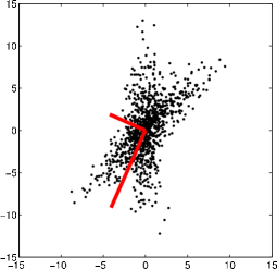
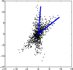
Figure 1: Comparison of singular vectors (left, scaled, in red) and DEIM-CUR columns (right, in blue) for a data set drawn from two multivariate normal distributions having different principal axes.

CUR-type factorizations originated with “pseudoskeleton” approximations [14] and pivoted, truncated QR decompositions [23]; in recent years many new algorithms have been proposed in the numerical linear algebra and theoretical computer science literatures. Some approaches seek to maximize the volume of the decomposition [14, 25]. Numerous other algorithms instead use leverage scores [5, 10, 22, 28]. These methods typically first compute a singular value decomposition ${\bf A}={\bf V}{\bf S}{\bf W}^{T}$ (or an approximation to it), with ${\bf V}\in\mbox{\Bb R}^{m\times n}$, ${\bf W}\in\mbox{\Bb R}^{n\times n}$.  The leverage score for the $j$th row ($k$th column) of ${\bf A}$ is the squared two-norm of the $j$th row of ${\bf V}$ ($k$th row of ${\bf W}$). When scaled by the number of singular vectors, these leverage scores give probability distributions for randomly sampling the columns and rows to form ${\bf C}$ and ${\bf R}$. This approach leads to probabilistic bounds on $\|{\bf A}-{\bf C}{\bf U}{\bf R}\|_{F}$ [10, 22]. In cases where ${\bf A}$ has small singular values (precisely the case where one would seek a low-rank factorization), the singular vectors can be sensitive to perturbations to ${\bf A}$, making the leverages scores unstable [18]. Thus leverage scores are often computed using only the leading few singular vectors, but the choice of how many vectors to keep can be somewhat ad hoc.

The algorithm described in Sections 2 and 3 is entirely deterministic and involves few (if any) parameters. The method is supported by an error analysis in Section 4 that also applies to a broad class of CUR factorizations. This section includes an improved bound on the error constants $\eta_{p}$ and $\eta_{q}$ for DEIM row and column selection, which also applies to the analysis of DEIM-based model order reduction [6]. In Section 5 we propose a novel incremental QR algorithm for approximating the SVD (and potentially also approximating leverage scores). Section 6 illustrates the performance of this new CUR factorization on several examples.

In many applications one cares primarily about key columns or rows of ${\bf A}$, rather than an explicit ${\bf A}={\bf C}{\bf U}{\bf R}$ factorization. The DEIM technique, which identifies rows and columns of ${\bf A}$ independently, can easily be used to select only columns or rows, leading to an “interpolatory decomposition” of the form ${\bf A}={\bf C}\widehat{{\bf U}}$ or ${\bf A}=\widehat{{\bf U}}{\bf R}$; such factorizations have the advantage that $\widehat{{\bf U}}$ can be much better conditioned than the ${\bf U}$ matrix in the CUR factorization. For further details about general interpolatory decompositions, see [7, §1].

2 CUR Factorization

We are concerned with large matrices ${\bf A}\in\mbox{\Bb R}^{m\times n}$ that represent nearly low-rank data, which can therefore be expressed as

$${\bf A}={\bf C}{\bf U}{\bf R}+{\bf F},$$ (2.1)

with $\|{\bf F}\|$ small relative to $\|{\bf A}\|$.  The matrix ${\bf C}\in\mbox{\Bb R}^{m\times k}$ is formed by extracting $k$ columns from ${\bf A}$, and ${\bf R}\in\mbox{\Bb R}^{k\times n}$ from $k$ rows of ${\bf A}$. The selected row and column indices are stored in the vectors ${\bf p},{\bf q}\in\mbox{\Bb N}^{k}$, so that ${\bf C}={\bf A}(:,{\bf q})$ and ${\bf R}={\bf A}({\bf p},:)$. Our choice for ${\bf p}$ and ${\bf q}$ is guided by knowledge of the rank-$k$ SVD (or an approximation to it). Before detailing the method for selecting these indices, we discuss how, given ${\bf p}$ and ${\bf q}$, one should construct ${\bf U}$ so that ${\bf C}{\bf U}{\bf R}$ satisfies desirable approximation properties.

As motivation, suppose for the moment that ${\bf A}$ has exact rank $k$, and ${\bf C}$ and ${\bf R}$ are full-rank subsets of the columns and rows of ${\bf A}$.  Now let ${\bf Y}\in\mbox{\Bb R}^{m\times k}$ and ${\bf Z}\in\mbox{\Bb R}^{n\times k}$ be any matrices that satisfy ${\bf Y}^{T}{\bf C}={\bf R}{\bf Z}={\bf I}\in\mbox{\Bb R}^{k\times k}$. Then ${\bf C}{\bf Y}^{T}$ is a projector onto ${\rm Ran}({\bf C})={\rm Ran}({\bf A})$ and $({\bf Z}{\bf R})^{T}$ is a projector onto ${\rm Ran}({\bf R}^{T})={\rm Ran}({\bf A}^{T})$, where ${\rm Ran}(\cdot)$ denotes the range (column space). It follows that ${\bf C}{\bf Y}^{T}{\bf A}={\bf A}$ and $({\bf Z}{\bf R})^{T}{\bf A}^{T}={\bf A}^{T}$.   Putting ${\bf U}\equiv{\bf Y}^{T}{\bf A}{\bf Z}$ gives

$${\bf C}{\bf U}{\bf R}={\bf C}{\bf Y}^{T}{\bf A}{\bf Z}{\bf R}={\bf A}{\bf Z}{\bf R}={\bf A}.$$

Thus, any choice of ${\bf Y}$ and ${\bf Z}$ that satisfies ${\bf Y}^{T}{\bf C}={\bf R}{\bf Z}={\bf I}$ gives a ${\bf U}$ such that ${\bf C}{\bf U}{\bf R}$ exactly recovers ${\bf A}$.  In general different choices for ${\bf Y}$ and ${\bf Z}$ give different ${\bf U}={\bf Y}^{T}{\bf A}{\bf Z}$.

Now consider the general case (2.1). Once ${\bf p}$, ${\bf q}$, ${\bf Y}$, and ${\bf Z}$ have been specified, then

$${\bf U}={\bf Y}^{T}{\bf A}{\bf Z}\quad{\rm and}\quad{\bf F}\equiv{\bf A}-{\bf C}{\bf U}{\bf R}.$$

One might design ${\bf Y}$ and ${\bf Z}$ so that ${\bf C}{\bf U}{\bf R}$ matches the selected columns ${\bf C}={\bf A}(:,{\bf q})$ and rows ${\bf R}={\bf A}({\bf p},:)$ of ${\bf A}$ exactly. This can be accomplished with interpolatory projectors, which we discuss in detail in the next section. For now, let ${\bf P}={\bf I}(\mkern 1.0mu:\mkern 1.0mu,{\bf p})\in\mbox{\Bb R}^{m\times k}$ and ${\bf Q}={\bf I}(\mkern 1.0mu:\mkern 1.0mu,{\bf q})\in\mbox{\Bb R}^{n\times k}$ be submatrices of the identity, so that ${\bf P}^{T}{\bf a}={\bf a}({\bf p})$ and ${\bf b}^{T}{\bf Q}={\bf b}({\bf q})^{T}$ for arbitrary vectors ${\bf a}$ and ${\bf b}$ of appropriate dimensions. Now define ${\bf Y}^{T}=({\bf P}^{T}{\bf C})^{-1}{\bf P}^{T}$ and ${\bf Z}={\bf Q}({\bf R}{\bf Q})^{-1}$ (presuming ${\bf P}^{T}{\bf C}$ and ${\bf R}{\bf Q}$ are invertible). Then since ${\bf C}={\bf A}(:,{\bf q})$ and ${\bf R}={\bf A}({\bf p},:)$,

$${\bf P}^{T}{\bf C}={\bf C}({\bf p},:)={\bf A}({\bf p},{\bf q})\quad\mbox{and}\quad{\bf R}{\bf Q}={\bf R}(:,{\bf q})={\bf A}({\bf p},{\bf q}),$$

so

$${\bf U}={\bf Y}^{T}{\bf A}{\bf Z}=({\bf P}^{T}{\bf C})^{-1}{\bf P}^{T}{\bf A}{\bf Q}({\bf R}{\bf Q})^{-1}={\bf A}({\bf p},{\bf q})^{-1}{\bf A}({\bf p},{\bf q}){\bf A}({\bf p},{\bf q})^{-1}={\bf A}({\bf p},{\bf q})^{-1}.$$

This CUR approximation matches the ${\bf q}$ columns and ${\bf p}$ rows of ${\bf A}$,

$${\bf A}(:,{\bf q})={\bf C}{\bf U}{\bf R}(:,{\bf q})\ \ {\rm and}\ \ {\bf A}({\bf p},:)={\bf C}({\bf p},:){\bf U}{\bf R},$$

and, in our experiments, usually delivers a very good approximation. However, a CUR factorization with better theoretical approximation properties results from orthogonal projection, as originally suggested by Stewart [23, p. 320]; see also, e.g., Mahoney and Drineas [22]. Given a selection of indices ${\bf p}$ and ${\bf q}$, again put

$${\bf C}={\bf A}(:,{\bf q})\quad\mbox{and}\quad{\bf R}={\bf A}({\bf p},:).$$

Assume that ${\bf C}$ and ${\bf R}$ both have full rank $k$, and now let ${\bf Y}^{T}={\bf C}^{I}\equiv({\bf C}^{T}{\bf C})^{-1}{\bf C}^{T}$ and ${\bf Z}={\bf R}^{I}\equiv{\bf R}^{T}({\bf R}{\bf R}^{T})^{-1}$ denote left and right inverses of ${\bf C}$ and ${\bf R}$. These choices also satisfy ${\bf Y}^{T}{\bf C}={\bf I}$ and ${\bf R}{\bf Z}={\bf I}$, but now ${\bf C}{\bf Y}^{T}={\bf C}{\bf C}^{I}$ and ${\bf Z}{\bf R}={\bf R}^{I}{\bf R}$ are orthogonal projectors. We compute

$${\bf U}={\bf Y}^{T}{\bf A}{\bf Z}={\bf C}^{I}{\bf A}{\bf R}^{I},$$

yielding a CUR factorization that can be viewed as a two step process: first the columns of ${\bf A}$ are projected onto Ran(${\bf C}$), then the result is projected onto the row space of ${\bf R}$:

$$1)\ \ {\bf M}={\bf C}{\bf C}^{I}{\bf A},\quad 2)\ \ {\bf C}{\bf U}{\bf R}={\bf M}{\bf R}^{I}{\bf R}.$$

Both steps are optimal with respect to the 2-norm error, which is the primary source of the excellent approximation properties of this approach.

Several strategies for selecting ${\bf p}$ and ${\bf q}$ have been proposed. The approach presented in the next section is simple to implement and has complexity $m\mkern 1.0muk$ and $n\mkern 1.0muk$ to select the indices ${\bf p}$ and ${\bf q}$, provided the leading $k$ right and left singular vectors of ${\bf A}$ are available. Thus the overall complexity is dominated by the construction of the rank-$k$ SVD ${\bf A}\approx{\bf V}{\bf S}{\bf W}^{T}$, where ${\bf V}^{T}{\bf V}={\bf W}^{T}{\bf W}={\bf I}\in\mbox{\Bb R}^{k\times k}$ and ${\bf S}={\rm diag}(\sigma_{1},\sigma_{2},\ldots,\sigma_{k})$ is the $k\times k$ matrix of dominant singular values $\sigma_{1}\geq\sigma_{2}\geq\cdots\geq\sigma_{k}$.

3 DEIM

The DEIM point selection algorithm was first presented in [6] in the context of model order reduction for nonlinear dynamical systems, and is a discrete variant of the Empirical Interpolation Method originally proposed in [4]. The DEIM procedure operates on the singular vector matrices ${\bf V}$ and ${\bf W}$ independently to select the row indices ${\bf p}$ and column indices ${\bf q}$. We explain the process for selecting ${\bf p}$; applying the same steps to ${\bf W}$ yields ${\bf q}$. To derive the method, we elaborate upon the interpolatory projectors introduced in the last section.

Definition 3.1

Given a full rank matrix ${\bf V}\in\mbox{\Bb R}^{m\times k}$ and a set of distinct indices ${\bf p}\in\mbox{\Bb N}^{k}$, the interpolatory projector for ${\bf p}$ onto ${\rm Ran}({\bf V})$ is

$${\cal P}\equiv{\bf V}({\bf P}^{T}{\bf V})^{-1}{\bf P}^{T},$$ (3.1)

where ${\bf P}={\bf I}(\mkern 1.0mu:\mkern 1.0mu,{\bf p})\in\mbox{\Bb R}^{m\times k}$, provided ${\bf P}^{T}{\bf V}$ is invertible.

In general ${\cal P}$ is an oblique projector, and it has an important property not generally enjoyed by orthogonal projectors: for any ${\bf x}\in\mbox{\Bb R}^{m}$,

$$({\cal P}{\bf x})({\bf p})\,=\,{\bf P}^{T}{\cal P}{\bf x}\,=\,{\bf P}^{T}{\bf V}({\bf P}^{T}{\bf V})^{-1}{\bf P}^{T}{\bf x}\,=\,{\bf P}^{T}{\bf x}\,=\,{\bf x}({\bf p}),$$

so the projected vector ${\cal P}{\bf x}$ matches ${\bf x}$ in the ${\bf p}$ entries, justifying the name “interpolatory projector.”

The DEIM algorithm processes the columns of

$${\bf V}=\left[\begin{array}[]{cccc}{\bf v}_{1}&{\bf v}_{2}&\cdots&{\bf v}_{k}\end{array}\right]$$

one at a time, starting from the leading singular vector ${\bf v}_{1}$. Each step processes the next singular vector to produce the next index. The first index $p_{1}$ corresponds to the largest magnitude entry in ${\bf v}_{1}$:

$$|{\bf v}_{1}(p_{1})|=\|{\bf v}_{1}\|_{\infty}.$$

Now define ${\bf p}_{1}\equiv[p_{1}]$, and let

$${\cal P}_{1}\equiv{\bf v}_{1}({\bf P}_{1}^{T}{\bf v}_{1})^{-1}{\bf P}_{1}^{T}$$

denote the interpolatory projector for ${\bf p}_{1}$ onto ${\rm Ran}({\bf v}_{1})$. The second index $p_{2}$ corresponds to the largest entry in ${\bf v}_{2}$, after the interpolatory projection in the ${\bf v}_{1}$ direction has been removed:

$${\bf r}_{2}\!\! \equiv \!\!{\bf v}_{2}-{\cal P}_{1}{\bf v}_{2}$$

$$|{\bf r}_{2}(p_{2})|\!\! = \!\!\|{\bf r}_{2}\|_{\infty}.$$

Notice that ${\bf r}_{2}(p_{1})=0$, since ${\cal P}_{1}{\bf v}_{2}$ matches ${\bf v}_{2}$ in the $p_{1}$ position, a consequence of interpolatory projection. This property ensures the process will never produce duplicate indices.

Now suppose we have $j-1$ indices, with

$${\bf p}_{j-1}\equiv\left[\begin{array}[]{c}p_{1}\\ \vdots\\ p_{j-1}\end{array}\right],\quad{\bf P}_{j-1}\equiv{\bf I}(\mkern 1.0mu:\mkern 1.0mu,{\bf p}_{j-1}),\quad{\bf V}_{j-1}\equiv[\begin{array}[]{ccc}{\bf v}_{1}&\cdots&{\bf v}_{j-1}\end{array}],\quad{\cal P}_{j-1}\equiv{\bf V}_{j-1}({\bf P}_{j-1}^{T}{\bf V}_{j-1})^{-1}{\bf P}_{j-1}^{T}.$$

To select $p_{j}$, remove from ${\bf v}_{j}$ its interpolatory projection onto indices ${\bf p}_{j-1}$ and take the largest remaining entry:

$${\bf r}_{j}\!\! \equiv \!\!{\bf v}_{j}-{\cal P}_{j-1}{\bf v}_{j}$$

$$|{\bf r}_{j}(p_{j})|\!\! = \!\!\|{\bf r}_{j}\|_{\infty}.$$

Implementations should not explicitly construct these projectors; see the pseudocode in Algorithm 1 for details.

Those familiar with partially pivoted LU decomposition will notice, on a moment’s reflection, that this index selection scheme is exactly equivalent to the index selection of partial pivoting. This arrangement is equivalent to the “left looking” variant of LU factorization [9, sect. 5.4], but with two important differences. First, there are no explicit row interchanges in DEIM, as there are in LU factorization. Second, the original basis vectors (columns of ${\bf V}$) are not replaced with the residual vectors, as happens in traditional LU decomposition. (In the context of model reduction, it is preferable to keep the nice orthogonal basis intact for use as a reduced basis.) We will exploit this connection with partially pivoted LU factorization to analyze the approximation properties of DEIM.

Since the DEIM algorithm processes the singular vectors sequentially, from most to least significant, it introduces new singular vector information in a coherent manner as it successively selects the $k$ indices. Contrast this to index selection strategies based on leverage scores, where all singular vectors are incorporated at once via row norms of ${\bf V}$ and ${\bf W}$; to account for the fact that higher singular vectors are less significant, such approaches often instead compute leverage scores using only a few of the leading singular vectors.

       Input: ${\bf V}$, an $m\times k$ matrix ($m\geq k$)    Output: ${\bf p}$, an integer vector with $k$ distinct entries in $\{1,\ldots,m\}$        ${\bf v}={\bf V}(:,1)$        $[\sim,p_{1}]={\rm max}(|{\bf v}|)$        ${\bf p}=[p_{1}]$        for $j=2,3,\ldots,k$        ${\bf v}={\bf V}(:,j)$        ${\bf c}={\bf V}({\bf p},1:j-1)^{-1}{\bf v}({\bf p})$        ${\bf r}={\bf v}-{\bf V}(:,1:j-1){\bf c}$        $[\sim,p_{j}]={\rm max}(|{\bf r}|)$        ${\bf p}=[{\bf p};\ p_{j}]$        end

Algorithm 1: DEIM point selection algorithm.

For the interpolatory projector ${\cal P}_{j}$ to exist at the $j$th step, ${\bf P}_{j-1}^{T}{\bf V}_{j-1}$ must be nonsingular. The linear independence of the columns of ${\bf V}$ assures this. In the following, ${\bf e}_{j}$ denotes the $j$th column of the identity matrix.

Lemma 3.1

Let ${\bf P}_{j}=[{\bf e}_{p_{1}},{\bf e}_{p_{2}},\ldots,{\bf e}_{p_{j}}]$ and let ${\bf V}_{j}=[{\bf v}_{1},{\bf v}_{2},\ldots,{\bf v}_{j}]$ for $1\leq j\leq k$. If ${{{\rm rank}\,}}({\bf V})=k$, then ${\bf P}_{j}^{T}{\bf V}_{j}$ is nonsingular for $1\leq j\leq k$.

Proof: Suppose ${\bf P}_{j-1}^{T}{\bf V}_{j-1}$ is nonsingular and let ${\bf r}_{j}={\bf v}_{j}-{\bf V}_{j-1}({\bf P}_{j-1}^{T}{\bf V}_{j-1})^{-1}{\bf P}_{j-1}^{T}{\bf v}_{j}.$ Then $\|{\bf r}_{j}\|_{\infty}>0$, for otherwise ${\bf 0}={\bf v}_{j}-{\bf V}_{j-1}{\bf c}_{j-1}$, in violation of the assumption that ${{{\rm rank}\,}}({\bf V})=k$. Thus

$$0<|{\bf e}_{p_{j}}^{T}{\bf r}_{j}|=|{\bf e}_{p_{j}}^{T}{\bf v}_{j}-{\bf e}_{p_{j}}^{T}{\bf V}_{j-1}({\bf P}_{j-1}^{T}{\bf V}_{j-1})^{-1}{\bf P}_{j-1}^{T}{\bf v}_{j}|,$$ (3.2)

where $p_{j}$ is the $j$th DEIM interpolation point. Now factor

$${\bf P}_{j}^{T}{\bf V}_{j}=\left[\begin{array}[]{cc}{\bf P}_{j-1}^{T}{\bf V}_{j-1}&{\bf P}_{j-1}^{T}{\bf v}_{j}\\ {\bf e}_{p_{j}}^{T}{\bf V}_{j-1}&{\bf e}_{p_{j}}^{T}{\bf v}_{j}\end{array}\right]=\left[\begin{array}[]{cc}{\bf I}_{j-1}&{\bf 0}\\ {\bf e}_{p_{j}}^{T}{\bf V}_{j-1}({\bf P}_{j-1}^{T}{\bf V}_{j-1})^{-1}&1\end{array}\right]\left[\begin{array}[]{cc}{\bf P}_{j-1}^{T}{\bf V}_{j-1}&{\bf P}_{j-1}^{T}{\bf v}_{j}\\ {\bf 0}&\nu_{j}\end{array}\right],$$ (3.3)

where

$$\nu_{j}={\bf e}_{p_{j}}^{T}{\bf v}_{j}-{\bf e}_{p_{j}}^{T}{\bf V}_{j-1}({\bf P}_{j-1}^{T}{\bf V}_{j-1})^{-1}{\bf P}_{j-1}^{T}{\bf v}_{j}.$$

The inequality (3.2) implies $\nu_{j}\neq 0$ and hence equation (3.3) implies ${\bf P}_{j}^{T}{\bf V}_{j}$ is nonsingular. Since ${\bf e}_{p_{1}}^{T}{\bf v}_{1}\neq 0$, this argument provides an inductive proof that ${\bf P}_{j}^{T}{\bf V}_{j}$ is nonsingular for $1\leq j\leq k$.  

4 CUR Approximation Properties

While the theory presented in this section was designed to bound $\|{\bf A}-{\bf C}{\bf U}{\bf R}\|$ for the DEIM-CUR method, the analysis applies to any CUR factorization with full rank ${\bf C}\in\mbox{\Bb R}^{m\times k}$ and ${\bf R}\in\mbox{\Bb R}^{k\times n}$, and ${\bf U}={\bf C}^{I}{\bf A}{\bf R}^{I}$, regardless of the procedure used for selecting the columns and rows.

Consider a CUR factorization that uses row indices ${\bf p}\in\mbox{\Bb N}^{k}$ and column indices ${\bf q}\in\mbox{\Bb N}^{k}$, and set

$${\bf P}={\bf I}(\mkern 1.0mu\mkern 1.0mu:\mkern 1.0mu\mkern 1.0mu,{\bf p})=[{\bf e}_{p_{1}},\ldots,{\bf e}_{p_{k}}]\in\mbox{\Bb R}^{m\times k},\qquad{\bf Q}={\bf I}(\mkern 1.0mu\mkern 1.0mu:\mkern 1.0mu\mkern 1.0mu,{\bf q})=[{\bf e}_{q_{1}},\ldots,{\bf e}_{q_{k}}]\in\mbox{\Bb R}^{n\times k}.$$

The first step in this analysis bounds the mismatch between ${\bf A}$ and its interpolatory projection ${\cal P}{\bf A}$.

Lemma 4.1

Assume ${\bf P}^{T}{\bf V}$ is invertible and let ${\cal P}={\bf V}({\bf P}^{T}{\bf V})^{-1}{\bf P}^{T}$ be the interpolatory projector $(\ref{eq:intproj})$. If ${\bf V}^{T}{\bf V}={\bf I}$, then any ${\bf A}\in\mbox{\Bb R}^{m\times n}$ satisfies

$$\|{\bf A}-{\cal P}{\bf A}\|\leq\|({\bf P}^{T}{\bf V})^{-1}\|\|({\bf I}-{\bf V}{\bf V}^{T}){\bf A}\|.$$

Additionally, if ${\bf V}$ consists of the leading $k$ left singular vectors of ${\bf A}$, then

$$\|{\bf A}-{\cal P}{\bf A}\|=\|({\bf I}-{\cal P}){\bf A}\|\leq\|({\bf P}^{T}{\bf V})^{-1}\|\,\sigma_{k+1}.$$

Proof: First note that ${\cal P}{\bf V}={\bf V}({\bf P}^{T}{\bf V})^{-1}{\bf P}^{T}{\bf V}={\bf V}$, so that $({\bf I}-{\cal P}){\bf V}={\bf 0}$. Therefore

$$\|{\bf A}-{\cal P}{\bf A}\|=\|({\bf I}-{\cal P}){\bf A}\|=\|({\bf I}-{\cal P})({\bf I}-{\bf V}{\bf V}^{T}){\bf A}\|\leq\|({\bf I}-{\cal P})\|\|({\bf I}-{\bf V}{\bf V}^{T}){\bf A}\|.$$

It is well known that

$$\|{\bf I}-{\cal P}\|=\|{\cal P}\|=\|({\bf P}^{T}{\bf V})^{-1}\|$$

so long as ${\cal P}\neq{\bf 0}\ {\rm or}\ {\bf I}$; see, e.g., [24]. This establishes the first result. The second follows from the fact that

$$\|({\bf I}-{\bf V}{\bf V}^{T}){\bf A}\|=\|{\bf A}-{\bf V}{\bf S}{\bf W}^{T}\|=\sigma_{k+1}$$

when ${\bf V}$ consists of the leading $k$ left singular vectors of ${\bf A}$.  

Now let ${\bf V}{\bf S}{\bf W}^{T}\approx{\bf A}$ be a rank-$k$ SVD of ${\bf A}$. (The singular vectors play a crucial role in this analysis, even if ${\bf p}$ and ${\bf q}$ were selected using some scheme that did not reference them.) In addition to the interpolatory projector ${\cal P}={\bf V}({\bf P}^{T}{\bf V})^{-1}{\bf P}^{T}$ that operates on the left of ${\bf A}$, we shall also use ${\cal Q}={\bf Q}({\bf W}^{T}{\bf Q})^{-1}{\bf W}^{T}$, which operates on the right of ${\bf A}$.  Assuming that ${\bf P}^{T}{\bf V}$ and ${\bf W}^{T}{\bf Q}$ are invertible, define the error constants

$$\eta_{p}\equiv\|({\bf P}^{T}{\bf V})^{-1}\|,\qquad\eta_{q}\equiv\|({\bf W}^{T}{\bf Q})^{-1}\|.$$

Lemma 4.1 implies

$$\|{\bf A}({\bf I}-{\cal Q})\|\leq\eta_{q}\mkern 1.0mu\mkern 1.0mu\sigma_{k+1}\quad{\rm and}\quad\|({\bf I}-{\cal P}){\bf A}\|\leq\eta_{p}\mkern 1.0mu\mkern 1.0mu\sigma_{k+1}.$$ (4.1)

The next lemma shows that these bounds on the error of the interpolatory projection of ${\bf A}$ onto the select columns and rows also apply to the orthogonal projections of ${\bf A}$ onto the same column and row spaces.

Lemma 4.2

Suppose the row and column indices ${\bf p}$ and ${\bf q}$ give full rank matrices ${\bf C}={\bf A}(\mkern 1.0mu\mkern 1.0mu:\mkern 1.0mu\mkern 1.0mu,{\bf q})={\bf A}{\bf Q}\in\mbox{\Bb R}^{m\times k}$ and ${\bf R}={\bf A}({\bf p},\mkern 1.0mu\mkern 1.0mu:\mkern 1.0mu\mkern 1.0mu)={\bf P}{\bf A}\in\mbox{\Bb R}^{k\times n}$, with finite error constants $\eta_{p}$ and $\eta_{q}$, and suppose that $k<\min\{m,n\}$. Then

$$\|({\bf I}-{\bf C}{\bf C}^{I}){\bf A}\|\leq\eta_{q}\mkern 1.0mu\mkern 1.0mu\sigma_{k+1}\quad{\rm and}\quad\|{\bf A}({\bf I}-{\bf R}^{I}{\bf R})\|\leq\eta_{p}\mkern 1.0mu\mkern 1.0mu\sigma_{k+1}.$$

Proof: Using the formula ${\bf C}={\bf A}{\bf Q}$, we have ${\bf C}^{I}=({\bf C}^{T}{\bf C})^{-1}{\bf C}^{T}=({\bf Q}^{T}{\bf A}^{T}{\bf A}{\bf Q})^{-1}({\bf A}{\bf Q})^{T}$, so the orthogonal projection of ${\bf A}$ onto ${\rm Ran}({\bf C})$ is

$${\bf C}{\bf C}^{I}{\bf A}=({\bf A}{\bf Q}({\bf Q}^{T}{\bf A}^{T}{\bf A}{\bf Q})^{-1}{\bf Q}^{T}{\bf A}^{T}){\bf A}={\bf A}({\bf Q}({\bf Q}^{T}{\bf A}^{T}{\bf A}{\bf Q})^{-1}{\bf Q}^{T}{\bf A}^{T}{\bf A}).$$

Hence the error in the orthogonal projection of ${\bf A}$ is

$$({\bf I}-{\bf C}{\bf C}^{I}){\bf A}={\bf A}({\bf I}-\mbox{\boldmath$\Phi$}),\ \ {\rm where}\ \ \mbox{\boldmath$\Phi$}={\bf Q}({\bf Q}^{T}{\bf A}^{T}{\bf A}{\bf Q})^{-1}{\bf Q}^{T}{\bf A}^{T}{\bf A}.$$ (4.2)

Note that $\Phi$ is an oblique projector onto ${\rm Ran}({\bf Q})$, so $\mbox{\boldmath$\Phi$}{\bf Q}={\bf Q}$. Therefore, $\mbox{\boldmath$\Phi$}{\cal Q}={\cal Q}$, since

$$\mbox{\boldmath$\Phi$}{\cal Q}=\mbox{\boldmath$\Phi$}{\bf Q}({\bf W}^{T}{\bf Q})^{-1}{\bf W}^{T}={\bf Q}({\bf W}^{T}{\bf Q})^{-1}{\bf W}^{T}={\cal Q}.$$

This implies that

$${\bf A}({\bf I}-\mbox{\boldmath$\Phi$})={\bf A}({\bf I}-\mbox{\boldmath$\Phi$})({\bf I}-{\cal Q})=({\bf I}-{\bf C}{\bf C}^{I}){\bf A}({\bf I}-{\cal Q}),$$

and so from (4.2) we have

$$\|({\bf I}-{\bf C}{\bf C}^{I}){\bf A}\| = \|{\bf A}({\bf I}-\mbox{\boldmath$\Phi$})\|$$

$$= \|({\bf I}-{\bf C}{\bf C}^{I}){\bf A}({\bf I}-{\cal Q})\|$$

$$\leq \|{\bf I}-{\bf C}{\bf C}^{I}\|\|{\bf A}({\bf I}-{\cal Q})\|$$

$$\leq \eta_{q}\mkern 1.0mu\mkern 1.0mu\sigma_{k+1}.$$

The last line follows from the bound (4.1) and the fact that $\|{\bf I}-{\bf C}{\bf C}^{I}\|=1$, since ${\bf C}{\bf C}^{I}$ is an orthogonal projector and $k<\min\{m,n\}$.

A similar argument shows that

$${\bf A}({\bf I}-{\bf R}^{I}{\bf R})=({\bf I}-\mbox{\boldmath$\Psi$}){\bf A}$$

where $\mbox{\boldmath$\Psi$}={\bf A}{\bf A}^{T}{\bf P}({\bf P}^{T}{\bf A}{\bf A}^{T}{\bf P})^{-1}{\bf P}^{T}$, and also that

$$({\bf I}-\mbox{\boldmath$\Psi$}){\bf A}=({\bf I}-{\cal P})({\bf I}-\mbox{\boldmath$\Psi$}){\bf A}=({\bf I}-{\cal P}){\bf A}({\bf I}-{\bf R}^{I}{\bf R}),$$

from which follows the error bound

$$\|{\bf A}({\bf I}-{\bf R}^{I}{\bf R})\|\leq\|({\bf I}-{\cal P}){\bf A}\|\|{\bf I}-{\bf R}^{I}{\bf R}\|\leq\eta_{p}\mkern 1.0mu\mkern 1.0mu\sigma_{k+1}.\qquad{{\hfill\rule{8.53581pt}{8.53581pt}}}$$

The main result on approximation of ${\bf A}$ by ${\bf C}{\bf U}{\bf R}$ readily follows from combining this last lemma with a basic CUR analysis technique used by Mahoney and Drineas [22, eq. (6)].

Theorem 4.1

Given ${\bf A}\in\mbox{\Bb R}^{m\times n}$ and $1\leq k<\min\{m,n\}$, let ${\bf C}={\bf A}(\mkern 1.0mu\mkern 1.0mu:\mkern 1.0mu\mkern 1.0mu,{\bf q})\in\mbox{\Bb R}^{m\times k}$ and ${\bf R}={\bf A}({\bf p},\mkern 1.0mu\mkern 1.0mu:\mkern 1.0mu\mkern 1.0mu)\in\mbox{\Bb R}^{k\times n}$ with finite error constants $\eta_{p}$ and $\eta_{q}$, and set ${\bf U}={\bf C}^{I}{\bf A}{\bf R}^{I}$. Then

$$\|{\bf A}-{\bf C}{\bf U}{\bf R}\|\leq(\eta_{p}+\eta_{q})\mkern 1.0mu\mkern 1.0mu\sigma_{k+1}.$$

Proof: From the definitions,

$${\bf A}-{\bf C}{\bf U}{\bf R}={\bf A}-{\bf C}{\bf C}^{I}{\bf A}{\bf R}^{I}{\bf R}=({\bf I}-{\bf C}{\bf C}^{I}){\bf A}+{\bf C}{\bf C}^{I}{\bf A}({\bf I}-{\bf R}^{I}{\bf R}).$$

Applying Lemma 4.2,

$$\|{\bf A}-{\bf C}{\bf U}{\bf R}\| \leq \|({\bf I}-{\bf C}{\bf C}^{I}){\bf A}\|+\|{\bf C}{\bf C}^{I}\|\|{\bf A}({\bf I}-{\bf R}^{I}{\bf R})\|$$

$$\leq \eta_{q}\mkern 1.0mu\mkern 1.0mu\sigma_{k+1}+\eta_{p}\mkern 1.0mu\mkern 1.0mu\sigma_{k+1}$$

$$= (\eta_{p}+\eta_{q})\mkern 1.0mu\mkern 1.0mu\sigma_{k+1},$$

since $\|{\bf C}{\bf C}^{I}\|=1$.  

Theorem 4.1 shows that ${\bf C}{\bf U}{\bf R}$ is within a factor of $\eta_{p}+\eta_{q}$ of the optimal rank-$k$ approximation, hence these error constants suggest a way to assess a wide variety of column/row selection schemes. The quality of the approximation is controlled by the conditioning of the selected $k$ rows of the dominant $k$ (exact) singular vectors. If those singular vectors are available as part of the column/row selection process, then Theorem 4.1 provides an a posteriori bound requiring only the fast (${\cal O}(k^{3})$) computation of $\eta_{p}$ and $\eta_{q}$, and thus could suggest methods for adjusting either $k$ or the point selection process to reduce the error constants. In this context, notice that if ${\bf V}{\bf S}{\bf W}^{T}$ is only an approximation to the optimal rank-$k$ SVD with ${\bf V}$ and ${\bf W}$ having orthonormal columns (as computed, for example, using the incremental QR algorithm described in the next section), the preceding analysis gives

$$\|{\bf A}-{\bf C}{\bf U}{\bf R}\|\!\! \leq \!\!\|({\bf I}-{\bf C}{\bf C}^{I}){\bf A}\|+\|{\bf A}({\bf I}-{\bf R}^{I}{\bf R})\|$$ (4.3)

$$= \!\!\|{\bf A}({\bf I}-{\cal Q})\|+\|({\bf I}-{\cal P}){\bf A}\|$$

$$\leq \!\!\|({\bf W}^{T}{\bf Q})^{-1}\|\|{\bf A}({\bf I}-{\bf W}{\bf W}^{T})\|+\|({\bf P}^{T}{\bf V})^{-1}\|\|({\bf I}-{\bf V}{\bf V}^{T}){\bf A}\|,$$

showing how $\sigma_{k+1}$ in Theorem 4.1 is replaced by the error in the approximate SVD through $\|{\bf A}({\bf I}-{\bf W}{\bf W}^{T})\|$ and $\|({\bf I}-{\bf V}{\bf V}^{T}){\bf A}\|$. In this case $\|({\bf W}^{T}{\bf Q})^{-1}\|$ and $\|({\bf P}^{T}{\bf V})^{-1}\|$ are computed using the approximate singular vectors in ${\bf V}$ and ${\bf W}$, rather than the exact singular vectors in the theorem. Alternatively, if one has probabilistic bounds for $\eta_{p}$ and $\eta_{q}$, then Theorem 4.1 immediately gives a probabilistic bound for $\|{\bf A}-{\bf C}{\bf U}{\bf R}\|$.

Numerical examples in Section 6 compare how the error constants evolve as $k$ increases for the DEIM-CUR factorization and several other factorizations based on leverage scores.

4.1 Interpretation of the bound for DEIM-CUR

For DEIM-CUR, we can ensure the hypotheses of Theorem 4.1 are satisfied and bound the error constants. Suppose the DEIM points are selected using the exact rank-$k$ SVD ${\bf A}\approx{\bf V}{\bf S}{\bf W}^{T}$.  Lemma 3.1 ensures that the matrices ${\bf P}^{T}{\bf V}$ and ${\bf W}^{T}{\bf Q}$ are invertible, so $\eta_{p}$ and $\eta_{q}$ are finite. The DEIM strategy also gives full rank ${\bf C}$ and ${\bf R}$ matrices, presuming $k\leq{\rm rank}({\bf A})$. To see this, note that for any unit vector ${\bf y}\in\mbox{\Bb R}^{k}$,

$${\bf C}{\bf y}={\bf A}{\bf Q}\mkern 1.0mu{\bf y}={\bf V}{\bf S}{\bf W}^{T}{\bf Q}\mkern 1.0mu{\bf y}+{\bf E}{\bf Q}\mkern 1.0mu{\bf y},$$

where ${\bf E}={\bf A}-{\bf V}{\bf S}{\bf W}^{T}$.  Since ${\bf V}^{T}{\bf E}={\bf 0},$

$$\|{\bf C}{\bf y}\|^{2}=\|{\bf A}{\bf Q}\mkern 1.0mu{\bf y}\|^{2}=\|{\bf V}{\bf S}{\bf W}^{T}{\bf Q}{\bf y}\|^{2}+\|{\bf E}{\bf Q}\mkern 1.0mu{\bf y}\|^{2}.$$

Since $\|{\bf W}^{T}{\bf Q}{\bf y}\|\geq\|{\bf y}\|/\|({\bf W}^{T}{\bf Q})^{-1}\|=1/\eta_{q}$,

$$\|{\bf C}{\bf y}\|\geq\|{\bf V}{\bf S}{\bf W}^{T}{\bf Q}{\bf y}\|\geq\sigma_{k}/\eta_{q}>0.$$

Thus ${\bf C}$ must be full rank. A similar argument shows ${\bf R}$ to be full rank as well.

The examples in Section 6 illustrate that $\eta_{p}$ and $\eta_{q}$ are often quite modest for the DEIM-CUR approach, e.g., ${\cal O}(100)$.   However, worst-case bounds permit significant growth in $k$ that is generally not observed in practice. We begin by stating a bound on this growth developed by Chaturantabut and Sorensen [6, Lemma 3.2].

Lemma 4.3

For the DEIM selection scheme derived above,

$$\eta_{p}\leq{(1+\sqrt{2m})^{k-1}\over\|{\bf v}_{1}\|_{\infty}},\qquad\eta_{q}\leq{(1+\sqrt{2n})^{k-1}\over\|{\bf w}_{1}\|_{\infty}},$$

where ${\bf v}_{1}$ and ${\bf w}_{1}$ denote the first columns of ${\bf V}$ and ${\bf W}$.

Motivated by recent work by Drmač and Gugercin [11] on a modified DEIM-like algorithm for model reduction, we can improve this bound considerably.

Lemma 4.4

For the DEIM selection scheme derived above,

$$\eta_{p}<\sqrt{mk\over 3}\ {2^{k}},\qquad\eta_{q}<\sqrt{nk\over 3}\ {2^{k}}.$$

Proof: We shall prove the result for $\eta_{p}$; the result for $\eta_{q}$ follows similarly. As usual, let ${\bf V}\in\mbox{\Bb R}^{m\times k}$ have orthonormal columns, and let ${\bf p}={\rm DEIM}({\bf V})$ denote the row index vector derived from the DEIM selection scheme described above. Let ${\bf P}={\bf I}(\,:\,,{\bf p})$ so that ${\bf P}^{T}{\bf V}={\bf V}({\bf p},\,:\,)$.

Without loss of generality, assume the DEIM index selection gives ${\bf p}=[1,2,\ldots,k]^{T}$. (Otherwise, introduce a permutation matrix to the argument that follows.) As described in section 3, the DEIM index selection is precisely the index selection of LU decomposition with partial pivoting, so one can write

$${\bf V}={\bf L}\kern 1.0pt{\bf T},$$

where the nonsingular matrix ${\bf T}\in\mbox{\Bb R}^{k\times k}$ is upper triangular and ${\bf L}\in\mbox{\Bb R}^{m\times k}$ is unit lower triangular with $|{\bf L}(i,j)|\leq 1$, ${\bf L}(j,j)=1,\ 1\leq j\leq k$ and ${\bf L}(i,j)=0,\ j>i$.

Let ${\bf L}_{1}\equiv{\bf L}(1:k,1:k)$. Then ${\bf V}({\bf p},\,:\,)={\bf L}_{1}{\bf T}$ and thus

$$\eta_{p}\equiv\|({\bf P}^{T}{\bf V})^{-1}\|=\|({\bf L}_{1}{\bf T})^{-1}\|\leq\|{\bf T}^{-1}\|\|{\bf L}_{1}^{-1}\|.$$

(The linear independence of the columns of ${\bf V}$ ensure that ${\bf L}_{1}$ and ${\bf T}$ are invertible.) Upper bounds for $\|{\bf T}^{-1}\|$ and $\|{\bf L}_{1}^{-1}\|$ will give an upper bound for $\eta_{p}$.

To bound $\|{\bf T}^{-1}\|$, let ${\bf y}\in\mbox{\Bb R}^{k}$ be a unit vector such that $\|{\bf T}^{-1}{\bf y}\|=\|{\bf T}^{-1}\|$. Then

$$\|{\bf T}^{-1}\|=\|{\bf T}^{-1}{\bf y}\|=\|{\bf V}{\bf T}^{-1}{\bf y}\|=\|{\bf L}{\bf y}\|.$$

Now

$$\|{\bf L}{\bf y}\|\leq\sqrt{m}\,\|{\bf L}{\bf y}\|_{\infty}=\sqrt{m}\,|{\bf e}_{j}^{T}{\bf L}{\bf y}|,$$

for some index $j\in\{1,\ldots,m\}$.  By the Cauchy–Schwarz inequality and the bound $|{\bf L}(i,j)|\leq 1$,

$$|{\bf e}_{j}^{T}{\bf L}{\bf y}|\leq\|{\bf L}^{T}{\bf e}_{j}\|\|{\bf y}\|\leq\sqrt{k}\cdot 1,$$

and so it follows that $\|{\bf T}^{-1}\|\leq\sqrt{mk}$.

The inverse of ${\bf L}_{1}$ can be bounded using forward substitution. Let ${\bf L}_{1}{\bf z}={\bf y}$, where $\|{\bf y}\|=1$ and $\|{\bf z}\|=\|{\bf L}_{1}^{-1}\|$. Forward substitution provides

$$\zeta_{1} = \gamma_{1}$$

$$\zeta_{i} = \gamma_{i}-\sum_{j=1}^{i-1}\lambda_{ij}\zeta_{j},\hbox to0.0pt{\qquad$i=2,\ldots,k$,\hss}$$

where $\zeta_{i}={\bf z}(i)$, $\gamma_{i}={\bf y}(i)$ and $\lambda_{ij}={\bf L}(i,j)$. We now use induction to prove

$$|\zeta_{i}|\leq 2^{i-1},\hbox to0.0pt{\qquad$1\leq i\leq k$.\hss}$$

First note that $\zeta_{1}=\gamma_{1}$, so $|\zeta_{1}|\leq|\gamma_{1}|\leq 1=2^{0}$ to establish the base case. Assume for some $i\geq 1$ that

$$|\zeta_{j}|\leq 2^{j-1},\hbox to0.0pt{\qquad$1\leq j\leq i$.\hss}$$

Then

$$|\zeta_{i+1}|=\bigg{|}\gamma_{i+1}-\sum_{j=1}^{i}\lambda_{ij}\zeta_{j}\bigg{|} \leq |\gamma_{i+1}|+\sum_{j=1}^{i}|\lambda_{ij}||\zeta_{j}|$$

$$\leq 1+\sum_{j=1}^{i}1\cdot 2^{j-1}=1+\sum_{j=0}^{i-1}2^{j}=1+(2^{i}-1)=2^{i}$$

to complete the induction. Now since $\|{\bf z}\|=\|{\bf L}_{1}^{-1}\|$,

$$\|{\bf L}_{1}^{-1}\|^{2}={\bf z}^{T}{\bf z}=\sum_{i=1}^{k}|\zeta_{i}|^{2}\leq\sum_{i=0}^{k-1}4^{i}=(4^{k}-1)/3.$$

Thus $\|{\bf L}_{1}^{-1}\|<2^{k}/\sqrt{3}$, which, together with the bound on the inverse of ${\bf T}$, provides the final result for $m>k$:

$$\eta_{p}\equiv\|({\bf P}^{T}{\bf V})^{-1}\|<\sqrt{mk\over 3}\,2^{k}.$$

If $m=k$, then $\eta_{p}=1$, and the result holds trivially.    

Note that this proof only relies on the orthonormality of the columns of ${\bf V}$ and ${\bf W}$, and hence it applies when the DEIM selection scheme is applied to approximate singular vectors, as in CUR error bound in (4.3).

Lemma 4.4 was inspired by the proof technique developed by Drmač and Gugercin [11] to bound $\|({\bf P}^{T}{\bf V})^{-1}\|$, when ${\bf P}$ is selected by applying a pivoted rank-revealing QR factorization scheme to ${\bf V}$.  Note that this new bound is on the same order of magnitude as the Drmač–Gugercin scheme. In practice, their scheme seems to give slightly smaller growth that is more consistent over a wide range of examples. Neither scheme experienced exponential growth over very extensive testing. For the DEIM approach, this absence of exponential growth is closely related to decades of experience with Gaussian elimination with partial pivoting. Element growth in ${\bf T}$ is bounded by a factor of $2^{k-1}$ (for a $k\times k$ matrix), and there is an example that achieves this growth. Nevertheless, this algorithm is almost exclusively used to solve linear systems because such growth is never experienced. Indeed, a similar near worst case example can be constructed for DEIM, although this growth has not been observed in practice.

A Growth Example: We now construct an orthonormal matrix ${\bf V}$ with the property

$${1\over\sqrt{8}}\ 2^{k}<\eta_{p}\equiv\|({\bf P}^{T}{\bf V})^{-1}\|<\sqrt{mk\over 3}\ 2^{k}$$ (4.4)

where ${\bf P}^{T}{\bf V}={\bf V}({\bf p},\,:\,)$ with ${\bf p}={\rm DEIM}({\bf V})$. To construct ${\bf V}$, begin by defining

$${\bf L}:=\left[\begin{array}[]{cccc}1&&&\\ -1&1&&\\ \vdots&\ddots&\ddots&\\ -1&\cdots&-1&1\\ -1&\cdots&-1&-1\\ \vdots&&&\vdots\\ -1&\cdots&-1&-1\end{array}\right]\in\mbox{\Bb R}^{m\times k}.$$

Now construct ${\bf V}{\bf T}_{1}\equiv{\bf L}$ as an economy-sized QR factorization of ${\bf L}$ (with no column pivoting). Since the columns of ${\bf L}$ are linearly independent by construction, ${\bf T}_{1}\in\mbox{\Bb R}^{k\times k}$ is invertible; define ${\bf T}\equiv{\bf T}_{1}^{-1}$, so that ${\bf V}={\bf L}\kern 1.0pt{\bf T}$. (Note that ${\bf T}$ plays the same role it does in the proof of Lemma 4.4.) If the DEIM procedure is applied to ${\bf V}$, then by construction ${\bf p}=[1,2,\ldots,k]$ (in exact arithmetic): during the DEIM procedure, the relations

$$\mbox{\boldmath$\ell$}_{j}\kern 1.0pt\tau_{jj}={\bf v}_{j}-{\bf V}_{j-1}({\bf P}_{j-1}^{T}{\bf V}_{j-1})^{-1}{\bf P}_{j-1}^{T}{\bf v}_{j},\hbox to0.0pt{\qquad$j>1$\hss}$$

hold, with $\mbox{\boldmath$\ell$}_{j}={\bf L}(\,:\,,j)$, $\tau_{jj}={\bf T}(j,j)$, ${\bf v}_{j}={\bf V}(\,:\,,j)$ , ${\bf P}_{j-1}={\bf I}(\,:\,,1:j-1)$ and ${\bf V}_{j-1}={\bf V}(\,:\,,1:j-1)$. Thus ${\bf p}(j)=j,\ j>1$ and it is easily seen that ${\bf p}(1)=1$.

Note that ${\bf V}{\bf T}^{-1}={\bf L}$ implies ${\bf T}^{-T}{\bf T}^{-1}={\bf L}^{T}{\bf L}$ hence $\|{\bf T}\|=1/\sigma_{k}$, where $\sigma_{k}$ is the smallest singular value of ${\bf L}$.  Let ${\bf y}$ be the corresponding right singular vector, so that

$$\sigma_{k}^{2}={\bf y}^{T}{\bf L}^{T}{\bf L}{\bf y}.$$

We claim that $\sigma_{k}\geq\sqrt{2}$.  To see this, write ${\bf L}$ in the form

$${\bf L}=\left[\begin{array}[]{c}{\bf I}_{k}\\ {\bf 0}\end{array}\right]-\left[\begin{array}[]{c}{\bf L}_{0}\\ {\bf E}\end{array}\right],$$

where

$${\bf I}_{k}=\left[\begin{array}[]{cccc}1\\ &1\\ &&\ddots\\ &&&1\end{array}\right],\quad{\bf L}_{0}=\left[\begin{array}[]{cccc}0\\ 1&\ddots\\ \vdots&\ddots&\ddots\\ 1&\cdots&1&0\end{array}\right],\quad{\bf E}=\left[\begin{array}[]{cccc}1&1&\cdots&1\\ 1&1&\cdots&1\\ \vdots&\vdots&\ddots&\vdots\\ 1&1&\cdots&1\end{array}\right]={\bf f}\kern 1.0pt{\bf e}^{T},$$

for ${\bf f}=[1,\ldots,1]^{T}\in\mbox{\Bb R}^{m-k}$.

$${\bf L}^{T}{\bf L} = {\bf I}_{k}-{\bf L}_{0}-{\bf L}_{0}^{T}+{\bf L}_{0}^{T}{\bf L}_{0}+{\bf E}^{T}{\bf E}$$

$$= {\bf I}_{k}-({\bf e}{\bf e}^{T}-{\bf I}_{k})+{\bf L}_{0}^{T}{\bf L}_{0}+(m-k){\bf e}{\bf e}^{T}$$

$$= 2\kern 1.0pt{\bf I}_{k}+{\bf L}_{0}^{T}{\bf L}_{0}+(m-k-1){\bf e}{\bf e}^{T}$$

$$= 2\kern 1.0pt{\bf I}_{k}+{\bf M},$$

where ${\bf M}:={\bf L}_{0}^{T}{\bf L}_{0}+(m-k-1){\bf e}{\bf e}^{T}$ is symmetric and positive semidefinite whenever $m>k$. Thus

$$\sigma_{k}^{2}={\bf y}^{T}{\bf L}^{T}{\bf L}{\bf y}={\bf y}^{T}(2{\bf I}_{k}+{\bf M}){\bf y}\geq 2$$

and hence it follows that

$$\|{\bf T}\|\leq 1/\sqrt{2}.$$

This implies

$$\|({\bf P}^{T}{\bf V})^{-1}\|=\|{\bf T}^{-1}{\bf L}_{1}^{-1}\|\geq\frac{\|{\bf L}_{1}^{-1}\|}{\|{\bf T}\|}\geq\sqrt{2}\ \|{\bf L}_{1}^{-1}\|.$$

To complete the lower bound, we must analyze $\|{\bf L}_{1}^{-1}\|$. Forward substitution gives ${\bf L}_{1}^{-1}{\bf e}_{1}=[1,1,2,4,\ldots,2^{k-2}]^{T}$ and thus

$$\|{\bf L}_{1}^{-1}\|>\|{\bf L}_{1}^{-1}{\bf e}_{1}\|=\sqrt{1+(4^{k-1}-1)/3}\ >2^{k-2}.$$

We arrive at the lower bound

$$\eta_{p}\equiv\|({\bf P}^{T}{\bf V})^{-1}\|\geq\sqrt{2}\ \|{\bf L}_{1}^{-1}\|\ >\sqrt{2}\cdot 2^{k-2},$$

and thus for this choice of ${\bf V}$, the DEIM error constant satisfies

$${1\over\sqrt{8}}\ 2^{k}<\eta_{p}<\sqrt{{mk\over 3}}\ 2^{k}.$$

This example is interesting because it relies on the behavior of the classic example for growth in LU decomposition [26, lecture 22]. However, in this case the pathological growth is caused by ${\bf L}$ and not by ${\bf T}$.

5 Incremental QR Factorization

The DEIM point selection process presumes access to the first $k$ left and right singular vectors of ${\bf A}\in\mbox{\Bb R}^{m\times n}$. If either $m$ or $n$ is of modest size (say ${}\leq 1000$) and ${\bf A}$ can be stored as a dense matrix,  library software for computing the “economy sized” SVD, e.g., [V,S,W] = svd(A,’econ’) in MATLAB, usually performs very well. For larger scale problems, the leading $k$ singular vectors can be computed using iterative methods, such as the Krylov subspace-based ARPACK software [21] (used by MATLAB’s svds command), PROPACK [20], IRLBA [1], or the Jacobi–Davidson algorithm [17]. Randomized SVD algorithms provide an appealing alternative with probabilistic error bounds [16]. Here we describe another approach that satisfies a deterministic error bound (Lemma 5.1) and only requires one pass through the matrix ${\bf A}$, a key property for massive data sets that cannot easily be stored in memory.

     Input: ${\bf A}$, an $m\times n$ matrix      tol, a positive scalar controlling the accuracy of the factorization    Output: ${\bf Q}$, an $m\times k$ matrix with orthonormal columns                ${\bf R}$, a $k\times n$ rectangular matrix                with ${\bf A}\approx{\bf Q}{\bf R}$        Choose $k\ll\min(m,n)$        Compute the QR factorization ${\bf A}(:,1:k)={\bf Q}{\bf R}$, with ${\bf Q}\in\mbox{\Bb R}^{n\times k}$ and ${\bf R}\in\mbox{\Bb R}^{k\times m}$        rownorms($i$) = $\|{\bf R}(i,:)\|^{2}$ for $i=1,\ldots,k$        $j=k+1$        while $j\leq n$        ${\bf a}={\bf A}(\mkern 1.0mu:\mkern 1.0mu,j);\ {\bf r}={\bf Q}^{T}{\bf a};\ \ {\bf f}={\bf a}-{\bf Q}{\bf r};\ \ \rho=\|{\bf f}\|;\ \ {\bf q}={\bf f}/\rho$        ${\bf Q}=[{\bf Q},\ {\bf q}];\ \ {\bf R}=\left[\begin{array}[]{cc}{\bf R}&{\bf r}\\ {\bf 0}&\rho\\ \end{array}\right]$        rownorms($i$) = rownorms($i$) + ${\bf r}(i)^{2}$ for $i=1,\ldots,k$        rownorms($k+1$) ${}=\rho^{2};\ \$        FnormR = sum(rownorms);        $[\sigma,i_{\rm min}]={\rm min}({\rm rownorms}(1:k+1));$        if $\sigma>({\it tol}^{2})*({\rm FnormR}-{\rm rownorms}(i_{\rm min})$        % no deflation        $k=k+1;$        else % deflation required        if $i_{\rm min}<k+1$        ${\bf R}(i_{\rm min},\mkern 1.0mu:\mkern 1.0mu)={\bf R}(k+1,\mkern 1.0mu:\mkern 1.0mu);\ {\bf Q}(\mkern 1.0mu:\mkern 1.0mu,i_{\rm min})={\bf Q}(\mkern 1.0mu:\mkern 1.0mu,k+1)$        $\ {\rm rownorms}(i_{min})={\rm rownorms}(k+1)$        end        % delete the minimum norm row of ${\bf R}$        ${\bf Q}={\bf Q}(\mkern 1.0mu:\mkern 1.0mu,1:k);{\bf R}={\bf R}(1:k,\mkern 1.0mu:\mkern 1.0mu)$        end        $j=j+1$        end

Algorithm 2: Incremental QR low rank approximate factorization

This approach is based on an incremental low rank ${\bf A}\approx{\bf Q}{\bf R}$ approximation, where ${\bf Q}\in\mbox{\Bb R}^{n\times k}$ has orthonormal columns and ${\bf R}\in\mbox{\Bb R}^{k\times m}$ is upper triangular. (In this section only, ${\bf Q}$ and ${\bf R}$ denote different quantities from elsewhere in the paper.) Take the dense (economy sized) SVD ${\bf R}=\widehat{{\bf V}}{\bf S}{\bf W}^{T}$, and put ${\bf V}={\bf Q}\widehat{{\bf V}}$ to get

$${\bf A}\approx{\bf Q}{\bf R}={\bf V}{\bf S}{\bf W}^{T}.$$ (5.1)

Incremental algorithms for building the QR factorization and SVD have been proposed by Stewart [23], Baker, Gallivan, and Van Dooren [2] and many others, as surveyed in [3]; these ideas are also closely related to rank-revealing QR factorizations [15]. Algorithm 2 differs from those of Stewart in its use of internal pivoting and threshold truncation in place of Stewart’s column pivoting. This distinction enables a one-pass algorithm that is closely related to [2, Algorithm 1].

The proposed method is presented in Algorithm 2, which proceeds at each step by orthogonalizing a column of ${\bf A}$ against the previously orthogonalized columns. The rank of the resulting factors is controlled through an update-and-delete procedure that is illustrated in Figure 2. After orthogonalizing a column of ${\bf A}$, the algorithm checks if any row of ${\bf R}$ has small relative norm; if such a row exists, the corresponding column of ${\bf Q}$ makes little contribution to the factorization, so that column of ${\bf Q}$ and row of ${\bf R}$ can be deleted at only a small loss of accuracy in the factorization. (Future columns of ${\bf A}$ will not be orthogonalized against the vector deleted from ${\bf Q}$, so this direction can re-emerge if a later column in ${\bf A}$ warrants it.)

Robust implementations of Algorithm 2 should replace the classical Gram–Schmidt operations

$${\bf r}={\bf Q}^{T}{\bf a},\ \ {\bf f}={\bf a}-{\bf Q}{\bf r}$$

with a re-orthogonalization step, as suggested by Daniel, Gragg, Kaufman, and Stewart [8]:

$${\bf r} = {\bf Q}^{T}{\bf a}$$

$${\bf f} = {\bf a}-{\bf Q}{\bf r}$$ (5.2)

$${\bf c}={\bf Q}^{T}{\bf f}$$

$${\bf f}={\bf f}-{\bf Q}{\bf c}$$ (5.3)

$${\bf r}={\bf r}+{\bf c}$$ (5.4)

$$\rho = \|{\bf f}\|$$

$${\bf q} = {\bf f}/\rho.$$

The extra steps (5.2)–(5.4) generally provide a ${\bf Q}$ that is numerically orthogonal to working precision. Pathological cases are easily overcome with some additional slight modifications; see [13] for a complete analysis. Because this algorithm uses the classical Gram–Schmidt method, one can easily block it for parallel efficiency.

Figure 2: Diagram illustrating the QR update procedure.

5.1 Incremental QR Error Bounds

At step $j$ the truncation criterion in Algorithm 2 will delete row ${\bf r}_{i}^{T}={\bf e}_{i}^{T}{\bf R}_{j}\$ if

$$\|{\bf r}_{i}\|\leq\mbox{{\it tol}}\,\|\widehat{{\bf R}}_{j}\|_{F},$$

where ${\bf r}_{i}^{T}$ is the row of minimum norm and $\widehat{{\bf R}}_{j}$ denotes ${\bf R}_{j}$ with the $i$th row deleted. This strategy has a straightforward error analysis, which, in light of the approximation (5.1), also implies an error bound on the resulting SVD.

Lemma 5.1

Let ${\bf R}_{j}$ be the triangular factor at step $j$ of Algorithm 2, and ${\bf Q}_{j}$ the corresponding orthonormal columns in the approximate QR factorization ${\bf A}_{j}\approx{\bf Q}_{j}{\bf R}_{j}$, where ${\bf A}_{j}$ consists of the first $j$ columns of ${\bf A}$. Then

$$\|{\bf A}_{j}-{\bf Q}_{j}{\bf R}_{j}\|_{F}\leq\mbox{{\it tol}}\cdot d_{j}\cdot\|{\bf R}_{j}\|_{F},$$

where $d_{j}$ is the number of coloumn/row deletions that have been made up to and including step $j$. (Note that ${\bf Q}_{j}\in\mbox{\Bb R}^{m\times(j-d_{j})}$, ${\bf R}\in\mbox{\Bb R}^{(j-d_{j})\times j}$, and $d_{n}=\min\{m,n\}-k$, where $k={{{\rm rank}\,}}({\bf Q}_{n}{\bf R}_{n})$.)

Before proving this lemma, we note that it gives a bound on the error in the resulting approximate SVD of ${\bf A}$. Suppose $d_{n}$ deletions are made when this algorithm computes the approximate factorization ${\bf A}\approx{\bf Q}{\bf R}$ with tolerance tol. Given the SVD ${\bf R}=\widehat{{\bf V}}{\bf S}{\bf W}^{*}$, set ${\bf V}\equiv{\bf Q}\widehat{{\bf V}}$. Then

$$\|{\bf A}-{\bf V}{\bf S}{\bf W}^{*}\|_{F}\leq\mbox{{\it tol}}\cdot d_{n}\cdot\|{\bf R}\|_{F}.$$

Proof of Lemma 5.1: The proof shall be by induction. Let ${\bf E}_{j}={\bf A}_{j}-{\bf Q}_{j}{\bf R}_{j}$ and assume

$$\|{\bf E}_{j}\|_{F}\leq\mbox{{\it tol}}\cdot d_{j}\cdot\|{\bf R}_{j}\|_{F}.$$ (5.5)

Orthogonalize column $j+1$ of ${\bf A}$ using Gram–Schmidt to obtain

$${\bf A}_{j+1}={\bf Q}_{j+1}{\bf R}_{j+1}+[{\bf E}_{j},{\bf 0}].$$

If no deflation occurs at this step, the bound holds trivially since

$$\|{\bf E}_{j+1}\|_{F}=\|[{\bf E}_{j},{\bf 0}]\|_{F}\leq tol\cdot d_{j}\cdot\|{\bf R}_{j}\|_{F}\leq\mbox{{\it tol}}\cdot d_{j+1}\cdot\|{\bf R}_{j+1}\|_{F},$$

because $d_{j+1}=d_{j}$ and $\|{\bf R}_{j}\|_{F}\leq\|{\bf R}_{j+1}\|_{F}$.

Suppose ${\bf R}_{j}$ has dimension $k\times j$ (i.e., $k=j-d_{j}$). Let $i$ be the index of the row of minimum norm and let $\widehat{{\bf R}}_{j+1}$ be obtained by deleting the $i$th row of ${\bf R}_{j+1}$.  If ${\bf r}_{i}^{T}={\bf e}_{i}^{T}{\bf R}_{j+1}$ satisfies $\|{\bf r}_{i}^{T}\|\leq tol\cdot\|\widehat{{\bf R}}_{j+1}\|_{F}$ then deflation occurs. Deleting column $i$ of ${\bf Q}_{j+1}$ and row $i$ of ${\bf R}_{j+1}$ replaces ${\bf Q}_{j+1}$ and ${\bf R}_{j+1}$ with $\widehat{{\bf Q}}_{j+1}$ and $\widehat{{\bf R}}_{j+1}$. Then

$$\widehat{{\bf Q}}_{j+1}\widehat{{\bf R}}_{j+1}={\bf Q}_{j+1}({\bf R}_{j+1}-{\bf e}_{i}{\bf r}_{i}^{T}),$$

and

$${\bf A}_{j+1}={\bf Q}_{j+1}({\bf R}_{j+1}-{\bf e}_{i}{\bf r}_{i}^{T})+[{\bf E}_{j},{\bf 0}]+{\bf Q}_{j+1}{\bf e}_{i}{\bf r}_{i}^{T}.$$

Hence the deletion gives the overall error

$${\bf E}_{j+1}={\bf A}_{j+1}-\widehat{{\bf Q}}_{j+1}\widehat{{\bf R}}_{j+1}=[{\bf E}_{j},{\bf 0}]+{\bf Q}_{j+1}{\bf e}_{i}{\bf r}_{i}^{T}.$$

Therefore, when $i<k+1$, the inductive assumption (5.5) implies

$$\|{\bf E}_{j+1}\|_{F}\leq\|{\bf E}_{j}\|_{F}+\|{\bf r}_{i}^{T}\|\leq\mbox{{\it tol}}\cdot(d_{j}\cdot\|{\bf R}_{j}\|_{F}+\|\widehat{{\bf R}}_{j+1}\|_{F})\leq\mbox{{\it tol}}\cdot(d_{j}+1)\cdot\|\widehat{{\bf R}}_{j+1}\|_{F},$$

since $\widehat{{\bf R}}_{j+1}$ contains row $k+1$ of ${\bf R}_{j+1}$, which must have a norm larger than the row marked for deletion. Since row $k+1$ of $\widehat{{\bf R}}_{j+1}$ consists of just one nonzero element,

$$\|\widehat{{\bf R}}_{j+1}\|^{2}_{F}\geq\|\widehat{{\bf R}}_{j}\|_{F}^{2}+\rho_{k+1,j+1}^{2}\geq\|{\bf R}_{j}\|_{F}^{2},$$

where $\rho_{k+1,j+1}$ is the element ${\bf R}_{j+1}(k+1,j+1)$ and $\widehat{{\bf R}}_{j}$ is the matrix ${\bf R}_{j}$ with $i$th row deleted. If $i=k+1$, then the last row of ${\bf R}_{j+1}$ is deleted and the desired inequality must hold, since ${\bf R}_{j}$ is a submatrix of $\widehat{{\bf R}}_{j+1}$. At the end of this process, replace ${\bf R}_{j+1}$ and ${\bf Q}_{j+1}$ with $\widehat{{\bf R}}_{j+1}$ and $\widehat{{\bf Q}}_{j+1}$ to obtain the approximation

$$\|{\bf A}_{j+1}\|\leq\mbox{{\it tol}}\cdot d_{j+1}\cdot\|{\bf R}_{j+1}\|_{F},$$

since $d_{j+1}=d_{j}+1$.

The error bound for the base case $j=1$ clearly holds, completing the induction.  

The approximate QR factorization that results from this algorithm could be used directly for the approximation of leverage scores. The perturbation theory of Ipsen and Wentworth [18] describes how the tolerance in our algorithm will affect the accuracy of the resulting leverage scores. We also note that for extra expediency this one-pass QR algorithm could be stopped when $\|\widehat{{\bf R}}_{j}\|_{F}\approx\|{\bf A}\|_{F}$ (at the cost of an extra pass through ${\bf A}$ to compute $\|{\bf A}\|_{F}$), or applied to only a random sampling of $k$ columns of ${\bf A}$. (Drmač and Gugercin propose a different random approach to DEIM index selection, based on sampling rows of ${\bf V}$ to compute DEIM indices [11].)

6 Computational Examples

This section presents some computational evidence illustrating the excellent approximation properties of the DEIM-CUR factorization, consistent with the error analysis in Section 4. For each of our three examples, we compare the accuracy of the DEIM-CUR factorization with several schemes based on leverage scores. To remove random variations from our experiments, in most cases we select columns and rows having the highest leverage scores; for the first example, we include results for random leverage score sampling. For Example 1 we also study the effect of inaccurate singular vectors on the DEIM selection, and compare the accuracy of DEIM-CUR to CUR approximations based on the column-pivoted QR algorithm.

Example 1. Low-rank approximation of a sparse, nonnegative matrix

The first example builds a matrix ${\bf A}\in\mbox{\Bb R}^{300,000\times 300}$ of the form

$${\bf A}=\sum_{j=1}^{10}{2\over j}\,{\bf x}_{j}{\bf y}_{j}^{T}+\sum_{j=11}^{300}{1\over j}\,{\bf x}_{j}{\bf y}_{j}^{T},$$ (6.1)

where ${\bf x}_{j}\in\mbox{\Bb R}^{300,000}$ and ${\bf y}_{j}\in\mbox{\Bb R}^{300}$ are sparse vectors with random nonnegative entries (in MATLAB, ${\bf x}_{j}={\tt sprand(300000,1,0.025)}$ and ${\bf y}_{j}={\tt sprand(300,1,0.025)}$). In this instantiation, ${\bf A}$ has 15,971,584 nonzeros, i.e., about 18% of all entries are nonzero. The form (6.1) is not a singular value decomposition, since $\{{\bf x}_{j}\}$ and $\{{\bf y}_{j}\}$ are not orthonormal sets; however, this decomposition suggests the structure of the SVD: the singular values decay like $1/j$, and with the first ten singular values weighted more heavily to give a notable drop between $\sigma_{10}$ and $\sigma_{11}$. We begin these experiments by computing ${\bf V}$ and ${\bf W}$ using MATLAB’s economy-sized SVD routine ([V,S,W] = svd(A,’0’)).

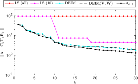
Figure 3: Accuracy of CUR approximations for the sparse, nonnegative matrix (6.1) using $k$ columns and rows, constructed by DEIM-CUR and two leverage score strategies: “LS (all)” selects rows and columns with highest leverage scores computed using all 300 singular vectors; “LS (10)” only uses the leading ten singular vectors. The “DEIM($\widehat{{\bf V}},\widehat{{\bf W}}$)” curve (nearly atop the “DEIM” curve) uses approximate singular vectors, described later.

Figure 3 compares the error $\|{\bf A}-{\bf C}{\bf U}{\bf R}\|$ for DEIM-CUR and methods that take ${\bf C}$ and ${\bf R}$ as the columns and rows of ${\bf A}$ with the highest leverage scores. These scores are computed using either all right and left singular vectors (300 of each), or using only the leading ten right and left singular vectors. Both approaches perform rather worse than DEIM-CUR, which closely tracks the optimal value $\sigma_{k+1}$.

To gain insight into these results, we examine the interpolation constants $\eta_{p}$ and $\eta_{q}$ for all three approaches. Figure 4 shows that these constants are largest for leverage scores based on all the singular vectors; using only ten singular vectors improves both the interpolation constants and the accuracy of the approximation (as seen in Figure 3). The DEIM-CUR method gives better interpolation constants and more accurate approximations.

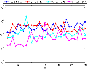
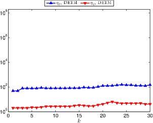
Figure 4: Error constants $\eta_{p}=\|({\bf P}_{k}^{T}{\bf V}_{k})^{-1}\|$ and $\eta_{q}=\|({\bf W}_{k}^{T}{\bf Q})^{-1}\|$ for rows and columns selected using two leverage score strategies (left plot) and the DEIM algorithm (right plot), for the matrix (6.1).

A CUR factorization can also be obtained by randomly sampling columns and rows of ${\bf A}$, with the probability of selection weighted by leverage scores [22]. We apply this approach on the current example, selecting $k=30$ rows and columns of ${\bf A}$ with a probability given by the leverage scores computed from the leading ten singular vectors (normalized to give a probability distribution). Figure 5 gives the results of ten independent experiments, showing that while sampling can sometimes yield better results than the deterministic leverage score approach, overall the approximations are still inferior to those from DEIM-CUR.

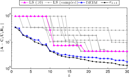
Figure 5: Accuracy of CUR approximations for (6.1) generated by randomly sampling rows and columns with probability weighted by leverage scores computed from the leading ten singular vectors. All ten trials (gray lines) perform similarly to the deterministic “LS (10)” approach, and worse than the DEIM-CUR approximation.

How robust is the DEIM-CUR approximation to errors in the singular vectors? To investigate, we compute $\widehat{{\bf V}}\approx{\bf V}$ and $\widehat{{\bf W}}\approx{\bf W}$ using the Incremental QR algorithm detailed in Section 5 (with ${\it tol}=10^{-4}$) and the Randomized SVD algorithm described by Halko, Martinsson, and Tropp [16, p. 227]. To give extreme examples of the latter, we compute $\widehat{{\bf V}}$ and $\widehat{{\bf W}}$ through only one or two applications each of ${\bf A}$ and ${\bf A}^{T}$. As Figure 6 illustrates, in both cases the angle between the exact and approximate leading singular subspaces is significant, particularly as $k$ grows. This drift in the subspaces has little effect on the accuracy of the DEIM approximations.

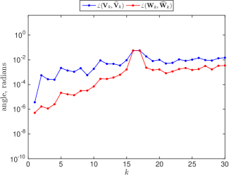
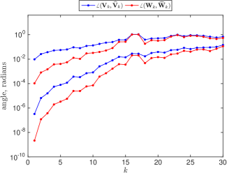
Figure 6: The angle between the leading $k$-dimensional exact singular subspaces ${\rm Ran}({\bf V}_{k})$ and ${\rm Ran}({\bf W}_{k})$ (generated by MATLAB’s svd command) and approximate singular subspaces ${\rm Ran}(\widehat{{\bf V}}_{k})$ and ${\rm Ran}(\widehat{{\bf W}}_{k})$ for the matrix (6.1). On the left, $\widehat{{\bf V}}_{k}$ and $\widehat{{\bf W}}_{k}$ are generated using the Incremental QR algorithm described in Section 5, with ${\it tol}=10^{-4}$; on the right, $\widehat{{\bf V}}_{k}$ and $\widehat{{\bf W}}_{k}$ are generated using randomized SVD algorithm [16] using one and two applications of ${\bf A}$ and ${\bf A}^{T}$.

• The DEIM approximation using the Incremental QR algorithm is quite robust, choosing at most 3 different row indices and 2 different column indices for $k=1,\ldots,30$, with a relative discrepancy in $\|{\bf A}-{\bf C}_{k}{\bf U}_{k}{\bf R}_{k}\|$ of at most 9.27% (and this realized only at step $k=30$).

• When ${\bf A}$ and ${\bf A}^{T}$ are applied once in the Randomized SVD algorithm, the DEIM indices differ considerably from those drawn from exact singular vectors (e.g., for $k=30$, 20 of 30 row indices and 3 of 30 column indices differ), yet the quality of the approximation $\|{\bf A}-{\bf C}_{k}{\bf U}_{k}{\bf R}_{k}\|$ remains almost the same (relative difference of at most 10.45%); see the dashed line in Figure 3.

• When ${\bf A}$ and ${\bf A}^{T}$ are applied twice, the DEIM indices are nearly identical (e.g., for $k=30$, 0 of 30 row indices and 2 of 30 column indices differ). On the scale of the plot in Figure 3, $\|{\bf A}-{\bf C}_{k}{\bf U}_{k}{\bf R}_{k}\|$ could not be distinguished from the DEIM-CUR errors using exact singular vectors; the maximum relative discrepancy is 2.21%.

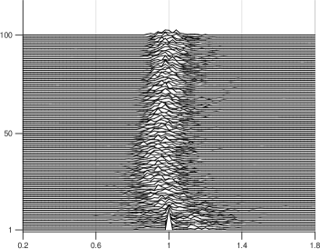
Figure 7: Comparison of DEIM-CUR and QR-CUR performance for 100 sparse random $300,000\times 300$ matrices of the form (6.1). The top plot shows a histogram of the ratio of $\|{\bf A}-{\bf C}_{k}{\bf U}_{k}{\bf R}_{k}\|$ for DEIM-CUR and QR-CUR. The bottom plots compare the error constant $\eta_{p}=\|({\bf P}_{k}^{T}{\bf V}_{k})^{-1}\|$ for DEIM-CUR (left) and QR-CUR (right); note the logarithmic scale of the horizontal axes in the lower plots.

Thus far we have only compared the DEIM-CUR approximations to CUR factorizations obtained from leverage scores, which also use singular vector information, thus illustrating how DEIM can use the same raw materials to better effect. Next we compare DEIM-CUR to approximations computed using a different approach based on QR factorization of ${\bf A}$; see, e.g., [7, 23]. Begin by computing a column-pivoted QR factorization of ${\bf A}$; the first $k$ selected columns give the indices ${\bf q}$, from which we extract ${\bf C}_{k}={\bf A}(\mkern 1.0mu\mkern 1.0mu:\mkern 1.0mu\mkern 1.0mu,{\bf q})$. Next, a column-pivoted QR factorization of ${\bf C}_{k}^{T}$ is performed; the first $k$ selected columns of ${\bf C}_{k}^{T}$ give the indices ${\bf p}$, from which we build ${\bf R}_{k}={\bf A}({\bf p},\mkern 1.0mu\mkern 1.0mu:\mkern 1.0mu\mkern 1.0mu)$. We refer to this technique as “QR-CUR.”

Figure 7 compares the results for 100 trials involving sparse random matrices of dimension $300,000\times 300$ having the form of our first experiment (6.1). DEIM-CUR and QR-CUR produce factorizations with similar accuracy, which we illustrate with a histogram of the ratio of $\|{\bf A}-{\bf C}_{k}{\bf U}_{k}{\bf R}_{k}\|$ for DEIM-CUR to QR-CUR, for $k=1,\ldots,100$. (DEIM-CUR produces a smaller error when the ratio is less than one.) While these errors are similar, the error constants $\eta_{p}$ and $\eta_{q}$ for the two methods are quite different. The bottom plots in Figure 7 compare histograms of $\log_{10}\eta_{p}$. For DEIM-CUR, the $\eta_{p}$ values are quite consistent across the 100 random ${\bf A}$, while for QR-CUR the $\eta_{p}$ values are both larger and rather less consistent. (The figures for $\eta_{q}$ are qualitatively identical, but about an order of magnitude smaller for both methods.)

The advantage of DEIM-CUR over approximations based on leverage scores remains when the singular values decrease more sharply. Modify (6.1) to give a more significant drop between $\sigma_{10}$ and $\sigma_{11}$:

$${\bf A}=\sum_{j=1}^{10}{1000\over j}\,{\bf x}_{j}{\bf y}_{j}^{T}+\sum_{j=11}^{300}{1\over j}\,{\bf x}_{j}{\bf y}_{j}^{T}.$$ (6.2)

As seen in Figures 8 and 9, the DEIM-CUR approach again delivers excellent approximations, while selecting the rows and columns with highest leverage scores does not perform nearly as well. (In Figure 9, note the significant jump in the “LS (10)” error constant $\eta_{q}$ corresponding to those $k$ values where $\|{\bf A}-{\bf C}_{k}{\bf U}_{k}{\bf R}_{k}\|/\sigma_{k+1}$ is large.)

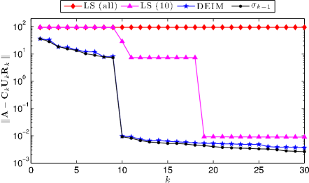
Figure 8: Accuracy of CUR approximations using $k$ rows and columns, for DEIM-CUR and two leverage score strategies for the sparse, nonnegative matrix (6.2). “LS (all)” selects rows and columns having the highest leverage scores computed using all 300 singular vectors; “LS (10)” uses the leading 10 singular vectors.

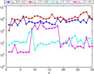
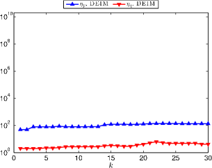
Figure 9: Error constants $\eta_{p}=\|({\bf P}_{k}^{T}{\bf V}_{k})^{-1}\|$ and $\eta_{q}=\|({\bf W}_{k}^{T}{\bf Q}_{k})^{-1}\|$ for rows and columns selected using two leverage score strategies (left plot) and the DEIM algorithm (right plot), for the sparse matrix ${\bf A}$ given in (6.2).

Example 2. TechTC term document data

The second example, adapted from Mahoney and Drineas [22], computes the CUR factorization of a term document matrix with data drawn from the Technion Repository of Text Categorization Datasets (TechTC) [12]. The rows of the data matrix correspond to websites (consolidated from multiple webpages), while the columns correspond to “features” (words from the text of the webpages). The $(j,k)$ entry of ${\bf A}$ reflects the importance of the feature text on the given website; most entries are zero. For this experiment we use TechTC-100 test set 26, which concatenates a data set relating to Evansville, Indiana (id 10567) with another for Miami, Florida (id 11346). Following Mahoney and Drineas [22], we omit all features with four or fewer characters from the data set, leaving a matrix with 139 rows and 15,170 columns. Each row of ${\bf A}$ is then scaled to have unit 2-norm. Ideally a CUR factorization not only gives an accurate low-rank approximation to ${\bf A}$, but also selects rows corresponding to representative webpages from each geographic area, and columns corresponding to meaningful features.

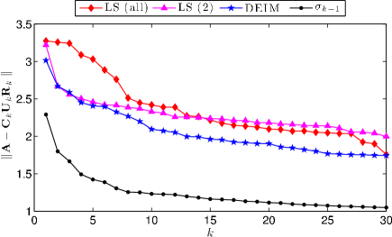
Figure 10: Accuracy of CUR factorizations for the TechTC example, selecting rows and columns using top leverage scores for all singular vectors and the leading two singular vectors, and DEIM.

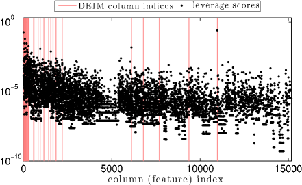
Figure 11: The columns selected by DEIM for the TechTC example, compared to leverage scores from the leading two singular vectors.

Figure 10 compares DEIM-CUR approximations to row and column selection based on highest leverage scores (from all singular vectors, or the two leading singular vectors). The DEIM-CUR approximations are typically more accurate than those based on leverage scores, but all approaches give errors roughly two times larger than the slowly-decaying optimal value of $\sigma_{k+1}$. How do the DEIM columns (features) compare to those with the highest leverage scores? Figure 11 shows the leverage scores associated with each column of ${\bf A}$ (based on the two leading singular vectors), along with the first 30 columns selected by DEIM. While the columns with highest leverage scores were found by DEIM, there are DEIM columns with marginal leverage scores, and vice versa. This data is more easily parsed in Table 1, which lists the features corresponding to the first 20 DEIM columns. (To ease comparison, we normalize leverage scores so that the maximum value is one.) The leading features identified by DEIM, including “evansville” (first DEIM point), “florida” (second), “miami” (sixth), and “indiana” (nineteenth), indeed reveal key geographic terms. These terms scored at least as high when ranked by leverage scores based on two leading singular vectors; when all singular vectors are used, the scores of these terms generally drop, relative to other features. Overall, one notes that DEIM selects a significantly different set of indices than those valued by leverage scores, and, as seen in Figure 10, tends to provide a somewhat better low-rank approximation.

Table 1: The features selected by DEIM-CUR for the TechTC data set, compared to the (scaled) leverage scores using the leading two singular vectors, and all singular vectors.

DEIM	index	LS (2)		LS (all)
rank	$q_{j}$	rank	score	rank	score	feature
1	10973	1	1.000	4	0.875	evansville
2	1	2	0.741	8	0.726	florida
3	1547	13	0.031	2	0.948	spacer
4	109	8	0.055	66	0.347	contact
5	209	12	0.040	32	0.458	service
6	50	4	0.116	6	0.739	miami
7	824	46	0.007	5	0.809	chapter
8	1841	33	0.010	20	0.537	health
9	171	5	0.113	13	0.617	information
10	234	16	0.026	37	0.436	events
11	595	84	0.004	15	0.576	church
12	60	15	0.026	67	0.347	email
13	945	10	0.047	30	0.474	services
14	1670	129	0.002	1	1.000	bullet
15	216	35	0.009	38	0.430	music
16	78	3	0.246	24	0.492	south
17	213	19	0.018	110	0.259	their
18	138	14	0.030	43	0.408	please
19	6110	7	0.060	95	0.280	indiana
20	1152	70	0.005	152	0.221	member

Example 3. Tumor detection in genetics data

Our final example uses the GSE10072 cancer genetics data set from the National Institutes of Health, previously investigated by Kundu, Nambirijan, and Drineas [19]. The matrix ${\bf A}\in\mbox{\Bb R}^{22,283\times 107}$ contains data for 22,283 probes applied to 107 patients. The $(j,k)$ entry of ${\bf A}$ reflects how strongly patient $k$ responded to probe $j$. This experiment seeks probes that segment the population into two clusters: the 58 patients with tumors, and the 49 without. To center the data, we subtract the mean of each row from all entries in that row. As shown in [19], the leading two principal vectors of this matrix segment the population very well.

Like the TechTC data, the singular values of ${\bf A}$ decay slowly, as seen in Figure 12. Once again the DEIM-CUR procedure produces a more accurate low-rank approximation than obtained by selecting the rows and columns with highest leverage scores, whether those are computed using all the singular vectors, or just the leading two or ten.

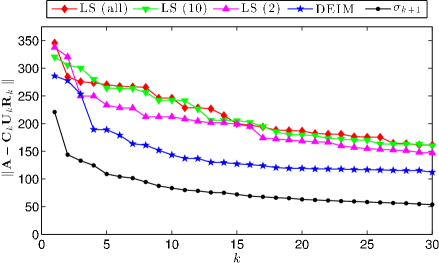
Figure 12: Accuracy of CUR factorizations for a genetics data set. DEIM-CUR consistently outperforms factorizations derived by taking the rows and columns with largest leverage scores, regardless of whether these scores are drawn from all singular vectors, the leading ten singular vectors, or the leading two singular vectors.

Table 2 reports the first 15 rows selected by the DEIM-CUR process, along with the corresponding leverage scores based on two, ten, and all singular vectors. Do the probes selected by DEIM discriminate the patients with tumors (“sick”) from those without (“well”)? To investigate, for each selected probe we count the number of large positive entries corresponding to sick and well patients. Some but not all of the DEIM-CUR probes effectively select only sick or well patients. Contrast these results with Table 3, which shows the probes with highest leverage scores (drawn from the leading two singular vectors). Only four of these probes were also selected by the DEIM procedure (even if we continue the DEIM procedure to select the maximum number, $n=107$, of indices). This discrepancy is quite different from the good agreement between DEIM and leverage score indices for the TechTC data in Table 1, despite the similar dimensions and the comparably slow decay of the singular values.

Table 2: Genetics example: the probes selected by DEIM-CUR, compared to the (scaled) leverage scores using the leading two singular vectors, ten singular vectors, and all singular vectors.

DEIM	index	probe	gene	number	number	LS (2)		LS (10)		LS (all)
rank	$q_{j}$	set	name	sick	well	rank	score	rank	score	rank	score
1	9565	210081_at	AGER	2	45	1	1.000	45	0.504	386	0.123
2	14270	214895_s_at	ADAM10	8	3	211	0.173	1171	0.108	3344	0.036
3	8650	209156_s_at	COL6A2	5	6	15156	0.005	252	0.245	708	0.091
4	11057	211653_x_at	AKR1C2	18	1	6440	0.017	11	0.656	146	0.185
5	14153	214777_at	IGKV4-1	27	3	281	0.148	19	0.607	106	0.209
6	18976	219612_s_at	FGG	17	17	2591	0.039	2	0.956	4	0.825
7	3831	204304_s_at	PROM1	16	4	992	0.073	70	0.417	32	0.345
8	3351	203824_at	TSPAN8	17	4	9687	0.011	21	0.582	31	0.355
9	4275	204748_at	PTGS2	18	14	424	0.118	13	0.624	42	0.313
10	1437	201909_at	RPS4Y1	21	34	8232	0.013	3	0.913	5	0.736
11	14150	214774_x_at	TOX3	34	0	95	0.262	49	0.492	102	0.210
12	10518	211074_at	FOLR1	7	4	9482	0.011	926	0.124	213	0.159
13	9580	210096_at	CYP4B1	6	44	8	0.797	65	0.431	54	0.284
14	4002	204475_at	MMP1	27	0	34	0.406	24	0.564	21	0.465
15	13990	214612_x_at	MAGEA	16	0	489	0.110	134	0.323	35	0.339

Table 3: Genetics example: the probes with top (scaled) leverage scores, derived from the first two singular vectors.

LS (2)	index	LS (2)	probe	gene	number	number	DEIM
rank	$q_{j}$	score	set	name	sick	well	rank
1	9565	1.000	210081_at	AGER	2	45	1
2	13766	0.922	214387_x_at	SFTPC	6	48	—
3	11135	0.907	211735_x_at	SFTPC	5	48	73
4	9361	0.899	209875_s_at	SPP1	50	2	—
5	5509	0.896	205982_x_at	SFTPC	5	48	—
6	9103	0.835	209613_s_at	ADH1B	2	47	—
7	14827	0.834	215454_x_at	SFTPC	0	46	—
8	9580	0.797	210096_at	CYP4B1	6	44	13
9	4239	0.754	204712_at	WIF1	5	43	70
10	3507	0.724	203980_at	FABP4	2	44	—
11	18594	0.717	219230_at	TMEM100	2	38	—
12	9102	0.684	209612_s_at	ADH1B	2	46	—
13	13514	0.626	214135_at	CLDN18	3	47	—
14	5393	0.626	205866_at	FCN3	0	39	—
15	4727	0.614	205200_at	CLEC3B	0	39	—

While the rows selected from leverage scores did not produce as accurate an approximation, $\|{\bf A}-{\bf C}_{k}{\bf U}_{k}{\bf R}_{k}\|$, as DEIM, these probes do a much more effective job of discriminating patients with tumors from those without. Indeed, for 14 of the top 15 probes, the tumor-free patients express strongly, while the patients with tumors do not; in the remaining case, the opposite occurs.

7 Conclusions

The Discrete Empirical Interpolation Method (DEIM) is an index selection procedure that gives simple, deterministic CUR factorizations of the matrix ${\bf A}$.  Since DEIM utilizes (approximate) singular vectors, we propose an effective one-pass incremental approximate QR factorization that can efficiently compute dominant singular vectors for data sets with rapidly decaying singular values; this method could prove useful in a variety of other settings. The accuracy of the resulting rank-$k$ CUR factorization can be bounded in terms of $\sigma_{k+1}$, the error in the best rank-$k$ approximation to ${\bf A}$.   Our analysis of the 2-norm error $\|{\bf A}-{\bf C}{\bf U}{\bf R}\|$ applies to all CUR approximations that use the optimal central factor ${\bf U}={\bf C}^{I}{\bf A}{\bf R}^{I}$, and hence can give insight into the performance of other index selection algorithms, such as leverage scores, uniform random sampling, or column-pivoted QR factorization. Numerical examples illustrate that the DEIM-CUR approach can deliver very good low rank approximations, compared to row selection based on dominant leverage scores.

References

- [1] James Baglama and Lothar Reichel. An implicitly restarted block Lanczos bidiagonalization method using Leja shifts. BIT, 53:285–310, 2013.
- [2] C. G. Baker, K. A. Gallivan, and P. Van Dooren. Low-rank incremental methods for computing dominant singular subspaces. Linear Algebra Appl., 436:2866–2888, 2012.
- [3] Christopher G. Baker. A block incremental algorithm for computing dominant singular subspaces. Master’s thesis, Florida State University, 2004.
- [4] Maxime Barrault, Yvon Maday, Ngoc Cuong Nguyen, and Anthony T. Patera. An ‘empirical interpolation’ method: application to efficient reduced-basis discretization of partial differential equations. Comptes Rendus Acad. Sci. Paris, Ser. I, 339:667–672, 2004.
- [5] Christos Boutsidis and David P. Woodruff. Optimal CUR matrix decompositions. arXiv:1405.7910 [cs.DS], 2014.
- [6] Saifon Chaturantabut and Danny C. Sorensen. Nonlinear model reduction via discrete empirical interpolation. SIAM J. Sci. Comput., 32:2737–2764, 2010.
- [7] H. Cheng, Z. Gimbutas, P. G. Martinsson, and V. Rokhlin. On the compression of low rank matrices. SIAM J. Sci. Comput., 26:1389–1404, 2005.
- [8] J. W. Daniel, W. B. Gragg, L. Kaufman, and G. W. Stewart. Reorthogonalization and stable algorithms for updating the Gram–Schmidt QR factorization. Math. Comp., 30:772–795, 1976.
- [9] Jack J. Dongarra, Iain S. Duff, Danny C. Sorensen, and Henk A. van der Vorst. Numerical Linear Algebra for High-Performance Computers. SIAM, Philadelphia, 1998.
- [10] Petros Drineas, Michael W. Mahoney, and S. Muthukrishnan. Relative-error CUR matrix decompositions. SIAM J. Matrix Anal. Appl., pages 844–881, 2008.
- [11] Zlatko Drmač and Serkan Gugercin. A new selection operator for the discrete empirical interpolation method — improved a priori error bound and extensions. arXiv:1505.0037 [cs.NA], 2015.
- [12] Evgeniy Gabrilovich and Shaul Markovitch. Text categorization with many redundant features: Using aggressive feature selection to make SVMs competitive with C4.5. In The 21st International Conference on Machine Learning (ICML), pages 321–328, 2004.
- [13] Luc Giraud, Julien Langou, Miroslav Rozložník, and Jasper van den Eshof. Rounding error analysis of the classical Gram–Schmidt orthogonalization process. Numer. Math., 101:87–100, 2005.
- [14] S. A. Goreinov, E. E. Tyrtyshnikov, and N. L. Zamarashkin. A theory of pseudoskeleton approximations. Linear Algebra Appl., 261:1–21, 1997.
- [15] Ming Gu and Stanley C. Eisenstat. Efficient algorithms for computing a strong rank-revealing QR factorization. SIAM J. Sci. Comput., 17:848–869, 1996.
- [16] N. Halko, P. G. Matinsson, and J. A. Tropp. Finding structure with randomness: probabilistic algorithms for constructing approximate matrix decompositions. SIAM Review, 53:217–288, 2011.
- [17] Michiel E. Hochstenbach. A Jacobi–Davidson type SVD method. SIAM J. Sci. Comput., 23:606–628, 2001.
- [18] Ilse C. F. Ipsen and Thomas Wentworth. Sensitivity of leverage scores. arXiv:1402.0957 [math.NA], 2014.
- [19] Abhisek Kundu, Srinivas Nambirajan, and Petros Drineas. Identifying influential entries in a matrix. arXiv:1310.3556 [cs.nA], 2013.
- [20] Rasmus Munk Larsen. PROPACK: Software for large and sparse SVD calculations. http://sun.stanford.edu/~rmunk/PROPACK/, 2005. Version 2.1.
- [21] R. B. Lehoucq, D. C. Sorensen, and C. Yang. ARPACK Users’ Guide: Solution of Large-Scale Eigenvalue Problems with Implicitly Restarted Arnoldi Methods. SIAM, Philadelphia, 1998.
- [22] Michael W. Mahoney and Petros Drineas. CUR matrix decompositions for improved data analysis. Proc. Nat. Acad. Sci., 106:697–702, 2009.
- [23] G. W. Stewart. Four algorithms for the efficient computation of truncated QR approximations to a sparse matrix. Numer. Math., 83:313–323, 1999.
- [24] Daniel B. Szyld. The many proofs of an identity on the norm of oblique projections. Numer. Alg., 42:309–323, 2006.
- [25] Christian Thurau, Kristian Kersting, and Christian Bauckhage. Deterministic CUR for improved large-scale data analysis: an empirical study. In Proceedings of the 2012 SIAM International Conference on Data Mining, pages 684–695, 2012.
- [26] Lloyd N. Trefethen and David Bau, III. Numerical Linear Algebra. SIAM, Philadelphia, 1997.
- [27] Lloyd N. Trefethen and Robert S. Schreiber. Average-case stability of Gaussian elimination. SIAM J. Matrix Anal. Appl., 11:335–360, 1990.
- [28] Shusen Wang and Zhihua Zhang. Improving CUR matrix decomposition and the Nyström approximation via adaptive sampling. J. Machine Learning Res., 14:2729–2769, 2013.