Raking the Cocktail Party

Abstract

We present the concept of an acoustic rake receiver—a microphone beamformer that uses echoes to improve the noise and interference suppression. The rake idea is well-known in wireless communications; it involves constructively combining different multipath components that arrive at the receiver antennas. Unlike spread-spectrum signals used in wireless communications, speech signals are not orthogonal to their shifts. Therefore, we focus on the spatial structure, rather than temporal. Instead of explicitly estimating the channel, we create correspondences between early echoes in time and image sources in space. These multiple sources of the desired and the interfering signal offer additional spatial diversity that we can exploit in the beamformer design.

We present several “intuitive” and optimal formulations of acoustic rake receivers, and show theoretically and numerically that the rake formulation of the maximum signal-to-interference-and-noise beamformer offers significant performance boosts in terms of noise and interference suppression. Beyond signal-to-noise ratio, we observe gains in terms of the perceptual evaluation of speech quality (PESQ) metric for the speech quality. We accompany the paper by the complete simulation and processing chain written in Python. The code and the sound samples are available online at http://lcav.github.io/AcousticRakeReceiver/.

I Introduction

Rake receivers take advantage of multipath propagation, instead of trying to mitigate it. The basic idea of the rake receivers (habitually used in wireless communications) is to coherently add the multipath components, and thus increase the effective signal-to-noise ratio ($\mathsf{SNR}$). The original scheme was developed for single-input-single-output systems [1], and it was later extended to arrays of antennas [2, 3] that exploit spatial diversity. By using antenna arrays and spatial processing, multipath components that would otherwise not be resolvable because they arrive at similar times, become resolvable because they arrive from different directions.

In spite of the success of the rake receivers in wireless communications, the principle has not received significant attention in room acoustics. Nevertheless, constructive use of echoes in rooms to improve beamforming has been mentioned in the literature [4, 5, 6]. In particular, the term acoustic rake receiver (ARR) was used in the SCENIC project proposal [4].

The list of ingredients for ARRs in room acoustics is similar as in wireless communications: a wave (acoustic instead of electromagnetic) propagates in space; reflections and scattering cause the wave to arrive at the receiver through multiple paths in addition to the direct path, and these multipath components all contain the source waveform.

The main difference is that in room acoustics we do not get to design the input signal. Spreading sequences used in CDMA are designed to be orthogonal to their shifts, which facilitates the multipath channel estimation; this orthogonality is not exhibited by speech. Moreover, speech segments are very long with respect to the time between the two consecutive echoes.

On the contrary, there are no significant differences in terms of the spatial structure. If we know where the echoes are coming from, we can design spatial processing algorithms—for example beamformers—that use multiple copies of the same signal arriving from different directions.

Imagine first that we know the room geometry. Then, if we localize the source, we can predict where its echoes will come from using simple geometric rules [7, 8]. Localizing the direct signal in a reverberant environment is a well-understood problem [9]. What is more, we do not need to know the room shape in detail—locations of the most important reflectors (ceiling, floor, walls) suffice to localize the major echoes. In many cases this knowledge is readily available from the floor plans or measurements. In ad-hoc deployments, the room geometry may be difficult to obtain. If that is the case, we can first perform a calibration step to learn it. An appealing method to infer the room geometry is by using sound, as was demonstrated recently [10, 11, 12, 13].

We may still be able to take advantage of the echoes without estimating the room geometry. Note that we are not after the room geometry itself; rather, we only need to know where the early echoes are coming from. Echoes can be seen as signals emitted by image sources—mirror images of the true source across reflecting walls [7]. Knowing where the echoes are coming from is equivalent to knowing where the image sources are.

Image source localization can be solved, for example, by echo sorting as described in [13]. Alternatively, O’Donovan, Duraiswami and Zotkin [5] propose to use an audio camera with a large number of microphones to find the images. Once the image sources are localized (in a calibration phase or otherwise), we can predict their movement using geometrical rules, as discussed in Section V. Thus, the acoustic raking is a multi-stage process comprising image source localization, tracking, and beamforming weight computation. The complete block diagram is shown in Fig. 1.

It is interesting to note the analogy between the ARRs and the human auditory perception. It is well established that the early echoes improve speech intelligibility [14, 15]. In fact, adding energy in the form of early echoes (approximately within the first 50 ms of the room impulse response (RIR)) is equivalent to adding the same energy to the direct sound [14]. This observation suggests new designs for indoor beamformers, with different choices of performance measures and reference signals. A related discussion of this topic is given by Habets and co-authors [16], who examine the tradeoff between dereverberation and denoising in beamforming. In addition to the standard $\mathsf{SNR}$, we propose to use the useful-to-detrimental ratio ($\mathsf{UDR}$), first defined by Lochner and Burger [15], and used by Bradley, Sato and Picard [14]. We generalize $\mathsf{UDR}$ to a scenario with interferers, defining it as the the ratio of the direct and early reflection energy to the energy of the noise and interference.

ARRs focus on the early part of the RIR, trying to concentrate the energy contained in the early echoes. In that regard, there are similarities between ARRs and channel shortening [17, 18]. Channel shortening produces filters that are much better behaved than complete inversion, e.g., by the multiple-input-output-theorem (MINT) [19, 20]. Nevertheless, it is assumed that we know the acoustic impulse responses between the sources and the microphones. In contrast to channel shortening, as well as other methods assuming this knowledge [21, 19], we never attempt the difficult task of estimating the impulse responses. Our task is simpler: we only need to detect the early echoes, and lift them to 3D space as image sources.

I-A Main Contributions and Limitations

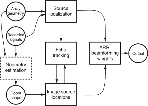
Figure 1: A block diagram for acoustic rake receivers. In this paper, we focus on ARR beamforming weight computation, and we briefly discuss echo tracking and image source localization. The geometry estimation block is optional (room geometry could be known in advance), hence the dashed box.

We introduce the acoustic rake receiver (ARR) as the echo-aware microphone beamformer. We present several formulations with different properties, and analyze their behavior theoretically and numerically. The analysis shows that ARRs lead to significantly improved $\mathsf{SNR}$ and interference cancellation when compared with standard beamformers that only extract the direct path. ARRs can suppress interference in cases when conventional beamforming is bound to fail, for example when an interferer is occluding the desired source (for a sneak-peak, fast forward to Fig. 6). We present optimal formulations that outperform the earlier delay-and-sum (DS) approaches [6], especially when interferers are present. Significant gains are observed not only in terms of signal-to-interference-and-noise ratio ($\mathsf{SINR}$) and $\mathsf{UDR}$, but also in terms of perceptual evaluation of speech quality (PESQ) [22].

The raking microphone beamformers are particularly well-suited to extracting the desired speech signal in the presence of interfering sounds, in part because they can focus on echoes of the desired sound and cancel the echoes of the interference. The analogous human capacity to focus on a particular acoustic stimulus while not perceiving other, unwanted sounds is called the cocktail party effect [23]. The title of this paper was inspired by that analogy.

We design and apply the ARRs in the frequency domain. Frequency domain formulation is simple and concise; it allows us to focus on objective gains from acoustic raking. Time-domain designs [24] offer better control over the impulse responses of the beamforming filters, but they are out of the scope of this paper. For a recent time-domain approach to ARR, see [25].

Let us also mention some limitations of our results. For clarity, the numerical experiments are presented in a 2D “room”, and as such are directly applicable to planar (e.g. linear or circular) arrays. Extension to 3D arrays is straightforward. We do not discuss robust formulations that address uncertainties in the array calibration. Microphones are assumed to be ideally omni-directional with a flat frequency response. Except for Section V, we assume that the locations of the image sources are known. We explain how to find the image sources when the room geometry is either known or unknown, but we do not provide a deep overview of the geometry estimation techniques. To this end, we suggest a number of references for the interested reader. We consider the walls to be flat-fading; in reality, they are frequency selective. We do not discuss the estimation of various covariance matrices [26].

The results in this paper are reproducible. Python (NumPy) [27] code for the beamforming routines, for the STFT processing engine, and to generate the figures and the sound samples is available online at http://lcav.github.io/AcousticRakeReceiver/.

I-B Paper Outline

In Section II we explain the notation and the signal model used in the paper. A brief overview of the relevant beamforming techniques and performance analysis is given in Section III. We formulate the acoustic rake receiver in Section IV, and we present a theoretical and numerical analysis of the corresponding beamformers. Section V explains how to locate the image sources, and comments on localizing the direct source. Numerical experiments are presented in Section VI.

II Notation and Signal model

We denote all matrices by bold uppercase letters, for example $\mathbf{A}$, and all vectors by bold lowercase letters, for example $\mathbf{x}$. The Hermitian transpose of a matrix or a vector is denoted by $(\,\cdot\,)^{H}$, as in $\mathbf{A}^{H}$, and the Euclidean norm of a vector by $\lVert\,\cdot\,\rVert$, that is, $\lVert\mathbf{x}\rVert\overset{\text{def}}{=}(\mathbf{x}^{H}\mathbf{x})^{\nicefrac{{1}}{{2}}}$.

Suppose that the desired source of sound is at the location $\mathbf{s}_{0}$ in a room. Sound from this source arrives at the microphones located at $[\mathbf{r}_{m}]_{m=1}^{M}$ via the direct path, but also via the echoes from the walls. The echoes can be replaced by the image sources—mirror images of the true sources across the corresponding walls—according to the image source model [7, 8]. An important consequence is that instead of modeling the source of the desired or the interefering signal as a single point in a room, we can model it as a collection of points in free space. A more detailed discussion of the image source model is given in Section V.

Denote the signal emitted by the source $\widetilde{x}[n]$ (e.g. the speech signal). Then all the image sources emit $\widetilde{x}[n]$ as well, and the signals from the image sources reach the microphones with the appropriate delays. In our application, the essential fact is that the echoes correspond to image sources. We denote the image source positions by $\mathbf{s}_{k}$, $1\leq k\leq K$, where $K$ denotes the largest number of image sources considered. Note that we do not care about the sequence of walls that generates $\mathbf{s}_{k}$, nor do we care about how many walls are in the sequence. For us, all $\mathbf{s}_{k}$ are simply additional sources of the desired signal. The described setup is illustrated Fig. 2.

Suppose further that there is an interferer at the location $\mathbf{q}_{0}$ (for simplicity, we consider only a single interferer). The interferer emits the signal $\widetilde{z}[n]$, and its image sources emit $\widetilde{z}[n]$ as well. Similarly as for the desired source, we denote by $\mathbf{q}_{k}$, $1\leq k\leq K^{\prime}$ the positions of the interfering image sources, with $K^{\prime}$ being the largest number of interfering image source considered. The model mismatch (e.g., the image sources of high orders and the late reverberation) and the noise are absorbed in the term $\widetilde{n}_{m}[n]$.

TABLE I: Summary of notation.

Symbol	Meaning
$M$	Number of microphones
$\mathbf{r}_{m}$	Location of the $m$th microphone
$\mathbf{s}_{0}$	Location of the desired source
$\mathbf{s}_{i}$	Location of the $i$th image of the desired source ($i\geq 1$)
$\mathbf{q}_{0}$	Location of the interfering source
$\mathbf{q}_{i}$	Location of the $i$th image of the interfering source ($i\geq 1$)
$x(\mathrm{e}^{\hskip 1.0ptj{\omega}})$	Spectrum of the sound from the desired source
$z(\mathrm{e}^{\hskip 1.0ptj{\omega}})$	Spectrum of the sound from the interfering source
$\mathbf{w}(\mathrm{e}^{\hskip 1.0ptj{\omega}})$	Vector of beamformer weights
$K$	Number of considered desired image sources
$K^{\prime}$	Number of considered interfering image sources
$a_{m}(\mathbf{s})$	$m$th component of the steering vector for a source at $\mathbf{s}$
$y_{m}$	Signal picked up by the $m$th microphone
$\|\,\cdot\,\|$	Euclidean norm, $\|\mathbf{x}\|=(\sum|x_{i}|^{2})^{\nicefrac{{1}}{{2}}}$.

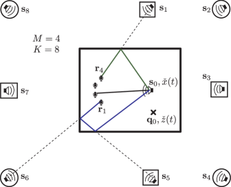
Figure 2: Illustration of the notation and concepts. Echoes of the desired signal emitted at $\mathbf{s}_{0}$ can be modeled as a direct sound coming from the image sources of $\mathbf{s}_{0}$. Two generations of image sources are illustrated: first ($\mathbf{s}_{1},\mathbf{s}_{3},\mathbf{s}_{5},\mathbf{s}_{7}$) and second ($\mathbf{s}_{2},\mathbf{s}_{4},\mathbf{s}_{6},\mathbf{s}_{8}$), as well as the corresponding sound rays for $\mathbf{s}_{5}$ and $\mathbf{s}_{6}$. The interferer is located at $\mathbf{q}_{0}$ (its image sources are not shown), and the microphones are located at $\mathbf{r}_{1},\ldots,\mathbf{r}_{4}$.

The signal received by the $m$th microphone is then a sum of convolutions

$$\widetilde{y}_{m}[n] =\sum_{k=0}^{K}\big{(}\widetilde{a}_{m}(\mathbf{s}_{k})\ast\widetilde{x}\big{)}[n]$$ (1)

$$+\sum_{k=0}^{K^{\prime}}\big{(}\widetilde{a}_{m}(\mathbf{q}_{k})\ast\widetilde{z}\big{)}[n]+\widetilde{n}_{m}[n],$$

where $\widetilde{a}_{m}(\mathbf{s}_{k})$ denotes the impulse response of the channel between the source located at $\mathbf{s}_{k}$ and the $m$th microphone—in this case a delay and a scaling factor.

We design and analyze all the beamformers in the frequency domain. That is, we will be working with the DTFT of the discrete-time signal $\widetilde{x}$,

$$x(\mathrm{e}^{\hskip 1.0ptj{\omega}})\overset{\text{def}}{=}\sum_{n\in\mathbb{Z}}\widetilde{x}[n]\,\mathrm{e}^{-j{\omega n}}.$$ (2)

In practical implementations, we use the discrete-time short-time Fourier transform (STFT). More implementation details are given in Section VI.

Using these notations, we can write the signal picked up by the $m$th microphone as

$$y_{m}(\mathrm{e}^{\hskip 1.0ptj{\omega}}) =\sum_{k=0}^{K}a_{m}(\mathbf{s}_{k},\Omega)x(\mathrm{e}^{\hskip 1.0ptj{\omega}})$$ (3)

$$+\sum_{k=0}^{K^{\prime}}a_{m}(\mathbf{q}_{k},\Omega)z(\mathrm{e}^{\hskip 1.0ptj{\omega}})+n_{m}(\mathrm{e}^{\hskip 1.0ptj{\omega}}),$$

where $n_{m}(\mathrm{e}^{\hskip 1.0ptj{\omega}})$ models the noise and other errors, and $a_{m}(\mathbf{s}_{k},\Omega)$ denotes the $m$th component of the steering vector for the source $\mathbf{s}_{k}$. The steering vector is the Fourier transform of the continuous version of the impulse response $\widetilde{a}(\mathbf{s}_{k})$, evaluated at the frequency $\Omega$. The discrete-time frequency $\omega$ and the continuous-time frequency $\Omega$ are related as $\omega=\Omega\,T_{s}$, where $T_{s}$ is the sampling period. The steering vector is then simply $\mathbf{a}(\mathbf{s}_{k},\Omega)=[a_{m}(\mathbf{s}_{k},\Omega)]_{m=0}^{M-1}$.

We can write out the entries of the steering vectors explicitly for a point source in free space. They are given as the appropriately scaled free-space Green’s functions for the Helmholtz equation [28],

$$a_{m}(\mathbf{s}_{k},\Omega)=\frac{\alpha_{k}}{4\pi\lVert\mathbf{r}_{m}-\mathbf{s}_{k}\rVert}\mathrm{e}^{-j{\kappa\lVert\mathbf{r}_{m}-\mathbf{s}_{k}\rVert}},$$ (4)

where we define the wavenumber as $\kappa\overset{\text{def}}{=}\Omega/c$, and $\alpha_{k}$ is the attenuation corresponding to $\mathbf{s}_{k}$.

Using vector notation, the microphone signals can be written concisely as

$$\mathbf{y}(\mathrm{e}^{\hskip 1.0ptj{\omega}})=\mathbf{A}_{s}(\mathrm{e}^{\hskip 1.0ptj{\omega}})\mathbf{1}x(\mathrm{e}^{\hskip 1.0ptj{\omega}})+\mathbf{A}_{q}(\mathrm{e}^{\hskip 1.0ptj{\omega}})\mathbf{1}z(\mathrm{e}^{\hskip 1.0ptj{\omega}})+\mathbf{n}(\mathrm{e}^{\hskip 1.0ptj{\omega}}),$$ (5)

where $\mathbf{A}_{s}(\mathrm{e}^{\hskip 1.0ptj{\omega}})\overset{\text{def}}{=}[\mathbf{a}(\mathbf{s}_{1},\Omega),\ldots,\mathbf{a}(\mathbf{s}_{K},\Omega)]$, $\mathbf{A}_{q}(\mathrm{e}^{\hskip 1.0ptj{\omega}})\overset{\text{def}}{=}[\mathbf{a}(\mathbf{q}_{1},\Omega),\ldots,\mathbf{a}(\mathbf{q}_{K^{\prime}},\Omega)]$, and $\mathbf{1}$ is the all-ones vector. From here onward, we suppress the frequency dependency of the steering vectors and the beamforming weights to reduce the notational clutter.

III Beamforming Preliminaries

Microphone beamformers combine the outputs of multiple microphones in order to achieve spatial selectivity, thereby suppressing noise and interference [29]. In the frequency domain, a beamformer forms a linear combination of the microphone outputs to yield the output $u$. That is,

$$u=\mathbf{w}^{H}\mathbf{y}=\mathbf{w}^{H}\mathbf{A}_{s}\mathbf{1}x+\mathbf{w}^{H}\mathbf{A}_{q}\mathbf{1}z+\mathbf{w}^{H}\mathbf{n},$$ (6)

where the vector $\mathbf{w}\in\mathbb{C}^{M}$ contains the beamforming weights.

The weights $\mathbf{w}$ are often selected so that they optimize some design criterion. Common examples of beamformers are the delay-and-sum (DS) beamformer, minimum-variance-distortionless-response (MVDR) beamformer, maximum-signal-to-interference-and-noise (Max-SINR) beamformer, and minimum-mean-squared-error (MMSE) beamformer. In this paper we discuss the rake formulation of the DS and the Max-SINR beamformers; for completeness, we first describe the non-raking variants.

III-A Delay-and-Sum Beamformer

DS is the simplest and often quite effective beamformer [29]. Assume that we want to listen to a source at $\mathbf{s}$. Then we form the the DS beamformer by compensating the propagation delays from the source $\mathbf{s}$ to the microphones $\mathbf{r}_{m}$,

$$u_{\text{DS}} =\frac{1}{M}\sum_{m=0}^{M-1}y_{m}\mathrm{e}^{\hskip 1.0ptj{\kappa\lVert\mathbf{r}_{m}-\mathbf{s}\rVert}}$$ (7)

$$\approx\frac{x}{4\pi\|\bar{\mathbf{r}}-\mathbf{s}\|}+\frac{1}{M}\sum_{m=0}^{M-1}n_{m},$$ (8)

where $\bar{\mathbf{r}}=\frac{1}{M}\sum_{m=0}^{M-1}\mathbf{r}_{m}$ denotes the center of the array. The beamforming weights can be read out from (7) as

$$\mathbf{w}_{\text{DS}}={\mathbf{a}(\mathbf{s})}\,\big{/}\,{\lVert\mathbf{a}(\mathbf{s})\rVert},$$ (9)

where we used the definition of $y_{m}$ (5) and the definition of the steering vector (4). We can see from (8) that if $\mathbf{n}\sim\mathcal{N}(\mathbf{0},\sigma^{2}\mathbf{I}_{M})$, then the output noise is distributed according to $\mathcal{N}(0,\sigma^{2}/M)$, that is, we obtain an $M$-fold decrease in the noise variance at the output with respect to any reference microphone.

III-B Maximum Signal-to-Interference-and-Noise Ratio Beamformer

The $\mathsf{SINR}$ is an important figure of merit used to assess the performance of ARRs, and to compare it with the standard non-raking beamformers. It is computed as the ratio of the power of the desired output signal to the power of the undesired output signal. The desired output signal is the output signal due to the desired source, while the undesired signal is the output signal due to the interferers and noise.

For a desired source at $\mathbf{s}$, and an interfering source at $\mathbf{q}$, we can write

$$\mathsf{SINR}\overset{\text{def}}{=}\frac{\mathbb{E}\left|\mathbf{w}^{H}\mathbf{a}(\mathbf{s})x\right|^{2}}{\mathbb{E}\left|\mathbf{w}^{H}(\mathbf{a}(\mathbf{q})z+\mathbf{n})\right|^{2}}=\sigma_{x}^{2}\frac{\mathbf{w}^{H}\mathbf{a}(\mathbf{s})\mathbf{a}(\mathbf{s})^{H}\mathbf{w}}{\mathbf{w}^{H}\mathbf{K}_{nq}\mathbf{w}},$$ (10)

where $\mathbf{K}_{nq}$ is the covariance matrix of the noise and the interference.

It is compelling to pick $\mathbf{w}$ that maximizes the $\mathsf{SINR}$ (10) [29]. The maximization can be solved by noting that the rescaling of the beamformer weights leaves the $\mathsf{SINR}$ unchanged. This means that we can minimize the denominator subject to numerator being an arbitrary constant. The solution is given as

$$\mathbf{w}_{\text{SINR}}=\frac{\mathbf{K}_{nq}^{-1}\mathbf{a}_{s}}{\mathbf{a}_{s}^{H}\mathbf{K}_{nq}^{-1}\mathbf{a}_{s}}.$$ (11)

Using the definition (10), we can derive the $\mathsf{SINR}$ for the Max-SINR beamformer as

$$\mathsf{SINR}=\sigma_{x}^{2}\mathbf{a}_{s}^{H}\mathbf{K}_{nq}^{-1}\mathbf{a}_{s}.$$ (12)

Because $\mathbf{K}_{nq}^{-1}$ is a Hermitian symmetric positive definite matrix, it has an eigenvalue decomposition as $\mathbf{K}_{nq}^{-1}=\mathbf{U}^{H}\mathbf{\Lambda}\mathbf{U}$, where $\mathbf{U}$ is unitary, and $\mathbf{\Lambda}$ is diagonal with positive entries. We can write $\mathbf{a}^{H}\mathbf{K}_{nq}^{-1}\mathbf{a}=(\mathbf{U}\mathbf{a})^{H}\mathbf{\Lambda}(\mathbf{U}\mathbf{a})$. Because $\lVert\mathbf{U}\mathbf{a}\rVert^{2}=\lVert\mathbf{a}\rVert^{2}$, and because $\mathbf{\Lambda}$ is positive, increasing $\lVert\mathbf{a}\rVert^{2}$ typically leads to an increased $\mathsf{SINR}$, although we can construct counterexamples. This will be important when we discuss the $\mathsf{SINR}$ gain of the Rake-Max-SINR beamformer.

IV Acoustic Rake Receiver

In this section, we present several formulations of the ARR. The Rake-DS beamformer is a straightforward generalization of the conventional DS beamformer. The one-forcing beamformer implements the idea of steering a fixed beam power towards every image source, while trying to minimize the interference and noise. The Rake-Max-SINR and Rake-Max-UDR beamformers optimize the corresonding performance measures; we show in Section VI that the Rake-Max-SINR beamforming performs best (except, as expected, in terms of $\mathsf{UDR}$).

IV-A Delay-and-Sum Raking

If we had access to every echo separately (i.e. not summed with all the other echoes), we could align them all to maximize the performance gain. Unfortunately, this is not the case: each microphone picks up the convolution of speech with the impulse response, which is effectively a sum of overlapping echoes of the speech signal. If we only wanted to extract the direct path, we would use the standard DS beamformer (9). To build the Rake-DS receiver, we create a DS beamformer for every image source, and average the outputs,

$$\frac{1}{K+1}\sum_{k=0}^{K}\frac{\alpha_{k}^{\prime}}{M}\sum_{m=0}^{M-1}y_{m}\mathrm{e}^{\hskip 1.0ptj{\kappa\lVert\mathbf{r}_{m}-\mathbf{s}_{k}\rVert}},$$ (13)

where $\alpha_{k}^{\prime}\overset{\text{def}}{=}\alpha_{k}/(4\pi\lVert\mathbf{r}_{m}-\mathbf{s}_{k}\rVert)$. We read out the beamforming weights from (13) as

$$\mathbf{w}_{\text{R-DS}}=\frac{1}{\lVert\sum_{k}\mathbf{a}(\mathbf{s}_{k})\rVert}\sum_{k=0}^{K}\mathbf{a}(\mathbf{s}_{k})=\frac{\mathbf{A}_{s}\mathbf{1}}{\lVert\mathbf{A}_{s}\mathbf{1}\rVert},$$ (14)

where we chose the scaling in analogy with (9) (scaling of the weights does not alter the output $\mathsf{SINR}$). It can be seen that this is just a scaled sum of the steering vectors for each image source.

IV-B One-Forcing Raking

A different approach, based on intuition, is to design a beamformer that listens to all $K$ image sources with the same power, and at the same time minimizes the noise and interference energy:

$$\operatorname*{minimize}_{\mathbf{w}\in\mathbb{C}^{M}}~{}\mathbb{E}\left|\sum_{k=0}^{K^{\prime}}\mathbf{w}^{H}\mathbf{a}(\mathbf{q}_{k})z+\mathbf{w}^{H}\mathbf{n}\right|^{2}$$ (15)

$$\text{subject to~{}}\mathbf{w}^{H}\mathbf{a}(\mathbf{s}_{k})=1,\forall~{}0\leq k\leq K.$$

Alternatively, we may choose to null the interfering source and its image sources. Both cases are an instance of the standard linearly-constrained-minimum-variance (LCMV) beamformer [30]. Collecting all the steering vectors in a matrix, we can write the constraint as $\mathbf{w}^{H}\mathbf{A}_{s}=\mathbf{1}^{T}$. The solution can be found in closed form as

$$\mathbf{w}_{\text{OF}}=\mathbf{K}_{nq}^{-1}\mathbf{A}_{s}(\mathbf{A}_{s}^{H}\mathbf{K}_{nq}^{-1}\mathbf{A}_{s})^{-1}\mathbf{1}_{M}.$$ (16)

A few remarks are in order. First, with $M$ microphones, it does not make sense to increase $K$ beyond $M$, as this results in more constraints than degrees of freedom. Second, using this beamformer is a bad idea if there is an interferer along the ray through the microphone array and any of image sources.

As with all LCMV beamformers, adding linear constraints uses up degrees of freedom that could otherwise be used for noise and interference suppression. It is better to let the “beamformer decide” or “the beamforming procedure decide” on how to maximize a well-chosen cost function; one such procedure is described in the next subsection.

TABLE II: Summary of beamformers.

Acronym	Description	Beamforming Weights
DS	Align delayed copies of signal at the microphone	$\mathbf{w}_{\text{DS}}={\mathbf{a}(\mathbf{s})}/{\lVert\mathbf{a}(\mathbf{s})\rVert}$
Max-SINR	$\text{max.~{}}{\mathbf{w}^{H}\mathbf{a}_{s}\mathbf{a}_{s}^{H}\mathbf{w}}/(\mathbf{w}^{H}\mathbf{K}_{nq}\mathbf{w})$	$\mathbf{w}_{\text{SINR}}={\mathbf{K}_{nq}^{-1}\mathbf{a}_{s}}/(\mathbf{a}_{s}^{H}\mathbf{K}_{nq}^{-1}\mathbf{a}_{s})$
Rake-DS	Weighted average of DS beamformers over image sources	$\mathbf{w}_{\text{R-DS}}={\mathbf{A}_{s}\mathbf{1}}/\lVert\mathbf{A}_{s}\mathbf{1}\rVert$
Rake-OF	$\text{min.~{}}\mathbb{E}\left|\sum_{k=0}^{K^{\prime}}\mathbf{w}^{H}\mathbf{a}(\mathbf{q}_{k})z+\mathbf{w}^{H}\mathbf{n}\right|^{2},\text{ s.t.~{}}\mathbf{w}^{H}\mathbf{A}_{s}=\mathbf{1}^{T}$	$\mathbf{w}_{\text{OF}}=\mathbf{K}_{nq}^{-1}\mathbf{A}_{s}(\mathbf{A}_{s}^{H}\mathbf{K}_{nq}^{-1}\mathbf{A}_{s})^{-1}\mathbf{1}_{M}$
Rake-Max-SINR	$\text{max.~{}}{\mathbb{E}\left|\sum_{k=0}^{K}\mathbf{w}^{H}\mathbf{a}(\mathbf{s}_{k})x\right|^{2}}\big{/}\ \mathbb{E}\left|\sum_{k=0}^{K^{\prime}}\mathbf{w}^{H}\mathbf{a}(\mathbf{q}_{k})z+\mathbf{w}^{H}\mathbf{n}\right|^{2}$	$\mathbf{w}_{\text{R-SINR}}={\mathbf{K}_{nq}^{-1}\mathbf{A}_{s}\mathbf{1}}/(\mathbf{1}^{H}\mathbf{A}_{s}^{H}\mathbf{K}_{nq}^{-1}\mathbf{A}_{s}\mathbf{1})$
Rake-Max-UDR	$\text{max.~{}}{\mathbb{E}\sum_{k=0}^{K}\left|\mathbf{w}^{H}\mathbf{a}(\mathbf{s}_{k})x\right|^{2}}\big{/}\ \mathbb{E}\left|\mathbf{w}^{H}\sum_{k=0}^{K^{\prime}}\mathbf{a}(\mathbf{q}_{k})z+\mathbf{w}^{H}\mathbf{n}\right|^{2}$	$\mathbf{w}_{\text{R-UDR}}=\mathbf{C}^{-1}\widetilde{\mathbf{w}}_{\text{max}}((\mathbf{C}^{-1})^{H}\mathbf{A}_{s}\mathbf{A}_{s}^{H}\mathbf{C}^{-1})$

IV-C Max-SINR Raking

The main workhorse of the paper is the Rake-Max-SINR. We compute the weights so as to maximize the $\mathsf{SINR}$, taking into account the echoes of the desired signal, and the echoes of the interfering signal,

$$\operatorname*{maximize}_{\mathbf{w}\in\mathbb{C}^{M}}~{}\frac{\mathbb{E}\left|\sum_{k=0}^{K}\mathbf{w}^{H}\mathbf{a}(\mathbf{s}_{k})x\right|^{2}}{\mathbb{E}\left|\sum_{k=0}^{K^{\prime}}\mathbf{w}^{H}\mathbf{a}(\mathbf{q}_{k})z+\mathbf{w}^{H}\mathbf{n}\right|^{2}}.$$ (17)

The logic behind this expression can be summarized as follows: we present the beamforming procedure with a set of good sources, whose influence we aim to maximize at the output, and with a set of bad sources, whose power we try to minimize at the output. Interestingly, this leads to the standard Max-SINR beamformer with a structured steering vector and covariance matrix. Define the combined noise and interference covariance matrix as

$$\mathbf{K}_{nq}\overset{\text{def}}{=}\mathbf{K}_{n}+\sigma_{z}^{2}\left(\sum_{k=0}^{K^{\prime}}\mathbf{a}(\mathbf{q}_{k})\right)\left(\sum_{k=0}^{K^{\prime}}\mathbf{a}(\mathbf{q}_{k})\right)^{H},$$ (18)

where $\mathbf{K}_{n}$ is the covariance matrix of the noise term, and $\sigma_{z}^{2}$ is the power of the interferer at a particular frequency.

Then the solution to (17) is given as

$$\mathbf{w}_{\text{R-SINR}}=\frac{\mathbf{K}_{nq}^{-1}\mathbf{A}_{s}\mathbf{1}}{\mathbf{1}^{H}\mathbf{A}_{s}^{H}\mathbf{K}_{nq}^{-1}\mathbf{A}_{s}\mathbf{1}}.$$ (19)

It is interesting to note that when $\mathbf{K}_{nq}=\sigma^{2}\mathbf{I}_{M}$ (e.g. no interferers and iid noise), the Rake-Max-SINR beamformer reduces to $\mathbf{A}_{s}\mathbf{1}/\lVert\mathbf{A}_{s}\mathbf{1}\rVert$, which is exactly the Rake-DS beamformer. This is analogous to the non-raking DS beamformer (9).

IV-D Max-UDR Raking

Finally, it is interesting to investigate what happens if we choose the weights that optimize the perceptually motivated $\mathsf{UDR}$ [14, 15]. The $\mathsf{UDR}$ expresses the fact that adding early reflections (up to 50 ms in the RIR) is as good as adding the energy to the direct sound in terms of speech intelligibility. The useful signal is a coherent sum of the direct and early reflected speech energy, so that

$$\mathsf{UDR}=\frac{\mathbb{E}\sum_{k=0}^{K}\left|\mathbf{w}^{H}\mathbf{a}(\mathbf{s}_{k})x\right|^{2}}{\mathbb{E}\left|\sum_{k=0}^{K^{\prime}}\mathbf{w}^{H}\mathbf{a}(\mathbf{q}_{k})z+\mathbf{w}^{H}\mathbf{n}\right|^{2}},$$ (20)

In applications $K$ is rarely large enough to cover all the reflections occurring within 50 ms, simply because it is too optimistic to assume we know all the corresponding image sources. Therefore, (20) typically underestimates the $\mathsf{UDR}$.

Alas, because (20) is specified in the frequency domain, it is challenging to control whether the reflections in the numerator arrive before or after the direct sound. Nevertheless, it is interesting to analyze it as it provides a basis for future work on time-domain raking formulations, and a meaningful evaluation of the raking algorithms presented in this paper.

To compute the Rake-Max-UDR weights, we solve the following program

$$\operatorname*{maximize}_{\mathbf{w}\in\mathbb{C}^{M}}\frac{\mathbb{E}\sum_{k=0}^{K}\left|\mathbf{w}^{H}\mathbf{a}(\mathbf{s}_{k})x\right|^{2}}{\mathbb{E}\left|\mathbf{w}^{H}\sum_{k=0}^{K^{\prime}}\mathbf{a}(\mathbf{q}_{k})z+\mathbf{w}^{H}\mathbf{n}\right|^{2}}.$$ (21)

This amounts to maximizing a particular generalized Rayleigh quotient,

$$\frac{\mathbf{w}^{H}\mathbf{A}_{s}\mathbf{A}_{s}^{H}\mathbf{w}}{\mathbf{w}^{H}\mathbf{K}_{nq}\mathbf{w}}.$$ (22)

Assuming that $\mathbf{K}_{nq}$ has a Cholesky decomposition as $\mathbf{K}_{nq}=\mathbf{C}^{H}\mathbf{C}$ we can rewrite the quotient (22) as

$$\frac{\widetilde{\mathbf{w}}^{H}(\mathbf{C}^{-1})^{H}\mathbf{A}_{s}\mathbf{A}_{s}^{H}\mathbf{C}^{-1}\widetilde{\mathbf{w}}}{\widetilde{\mathbf{w}}^{H}\widetilde{\mathbf{w}}},$$ (23)

where $\widetilde{\mathbf{w}}\overset{\text{def}}{=}\mathbf{C}\mathbf{w}$. The maximum of this expression is

$$\lambda_{\text{max}}((\mathbf{C}^{-1})^{H}\mathbf{A}_{s}\mathbf{A}_{s}^{H}\mathbf{C}^{-1}),$$ (24)

where $\lambda_{\text{max}}(\,\cdot\,)$ denotes the largest eigenvalue of the matrix in the argument. The maximum is achieved by the corresponding eigenvector $\widetilde{\mathbf{w}}_{\text{max}}$. Then the optimal weights are given as

$$\mathbf{w}_{\text{R-UDR}}=\mathbf{C}^{-1}\widetilde{\mathbf{w}}_{\text{max}}.$$ (25)

IV-E SINR Gain from Raking

Intuitively, if we have multiple sources of the desired signal scattered in space, and we account for it in the design, we should do at least as well as when we ignore the image sources. Let us see how large the gain can be for the Rake-Max-SINR beamformer. We have that

$$\mathsf{SINR}=(\mathbf{A}_{s}\mathbf{1})^{H}\mathbf{K}_{nq}^{-1}(\mathbf{A}_{s}\mathbf{1}).$$ (26)

Intuitively, the larger the norm of $\mathbf{A}_{s}\mathbf{1}$, the better the $\mathsf{SINR}$ (as $\mathbf{K}_{nq}$ is positive). To explicitly see if there is any gain in using the acoustic rake receiver, we should compare the standard Max-SINR beamformer with the Rake-Max-SINR, e.g., we should evaluate

$$\frac{\big{(}\sum_{k}\mathbf{a}(\mathbf{s}_{k})\big{)}^{H}\mathbf{K}_{nq}^{-1}\big{(}\sum_{k}\mathbf{a}(\mathbf{s}_{k})\big{)}}{\mathbf{a}(\mathbf{s}_{0})^{H}\mathbf{K}_{nq}^{-1}\mathbf{a}(\mathbf{s}_{0})}.$$ (27)

One possible interpretation of (27) is that we ask whether the steering vectors $\mathbf{a}(\mathbf{s}_{k})$ sum coherently or they cancel out.

To answer this, assume that $\mathbf{s}_{k}$, $0\leq k\leq K$ are the desired sources (true and image), and let $\beta\overset{\text{def}}{=}\sum_{k=1}^{K}(\alpha_{k}/\alpha_{0})^{2}$, where $\alpha_{k}$ is the strength of the source $\mathbf{s}_{k}$ received by the array. Then

$$\mathbb{E}\left(\left\|\sum_{k=0}^{K}\mathbf{a}(\mathbf{s}_{k})\right\|^{2}\right)\approx(1+\beta)\,\mathbb{E}(\lVert\mathbf{a}(\mathbf{s}_{0})\rVert^{2}),$$ (28)

that is, we can expect an increase in the output $\mathsf{SINR}$ approximately by a factor of $(1+\beta)$ when using the Rake-Max-SINR beamformer. This statement is made precise in Theorem 1 in the Appendix. It holds when $\mathbf{K}_{nq}$ has eigenvalues of similar magnitude, which is typically not the case in the presence of interferers. However, we show in Section VI that with interferers present, the gains actually increase.

A couple of remarks are in order:

1. This result is in expectation; it says that on average, the $\mathsf{SINR}$ will increase by a factor of $(1+\beta)$. In the worst case, the steering vectors $\mathbf{a}(\mathbf{s}_{k})$ can even cancel out so that the $\mathsf{SINR}$ decreases. But the numerical experiments suggest that this is very rare in practice, and we can on the other hand observe large gains.

2. We see that summing the phasors in $a_{m}(\mathbf{s}_{k})$ behaves as a two-dimensional random walk. It is known that the root-mean-square distance of a 2D random walk from the origin after $n$ steps is $\sqrt{n}$ [31].

3. Due to the far-field assumption in Theorem 1, the attenuations $\alpha_{k}$ are assumed to be independent of the microphones; in reality they do depend on the source locations. However, they also depend on a number of additional factors, for example wall attenuations and radiation patterns of the sources. Therefore, for simplicity, we consider them to be independent. One can verify that this assumption does not change the described trend.

It is reassuring to observe the behavior suggested by (28) in practice. Fig. 3 shows the comparison of the prediction by Theorem 1 with the $\mathsf{SNR}$ gains observed in simulated rooms. In this case, we are comparing the pure $\mathsf{SNR}$ gain for white noise, without interferers. To generate Fig. 3, we randomized the location of the source inside the rectangular room. For simplicity we fixed the signal power as received by the microphones to the same value for all the image sources, so that the expected gain is $K+1$ in the linear scale. The curves agree near-perfectly with the prediction of Theorem 1.

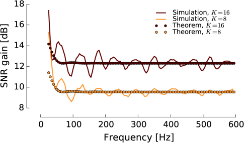
Figure 3: Comparison of the simulated $\mathsf{SNR}$ gains and the theoretical prediction from Theorem 1 for $K=8$, and $K=16$. The theoretical prediction of the gain is $10\log_{10}(8+1)\approx 9.54$ for $K=8$, and $10\log_{10}(16+1)\approx 12.30$ for $K=16$.

V Finding and tracking the echoes

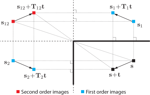
Figure 4: Illustration of image source tracking in rectangular geometries.

Thus far we assumed that the locations of the image sources are known. In this section we briefly describe some methods to localize them when they are a priori unknown. We assume that we can localize the true source, or at least one image source. Combined with the knowledge of the room geometry, this suffices to find the locations of other image sources [32].

V-A Known room geometry

In many cases, for example for fixed deployments, the room geometry is known. This knowledge could be obtained at the time of the deployment, or from blueprints. In most indoor environments, we encounter a large number of planar reflectors. These reflectors correspond to image sources. With reference to Fig. 4, we can easily compute the image source locations [7] (we note that the image source model is not limited to right angle geometries [8]).

Suppose that the real source is located at $\mathbf{s}$. Then the image source with respect to wall $i$ is computed as,

$$\mathbf{im}_{i}(\mathbf{s})=\mathbf{s}+2\left\langle\mathbf{p}_{i}-\mathbf{s},\mathbf{n}_{i}\right\rangle\mathbf{n}_{i},$$ (29)

where $i$ indexes the wall, $\mathbf{n}_{i}$ is the outward normal associated with the $i$th wall, and $\mathbf{p}_{i}$ is any point belonging to the $i$th wall. Analogously, we compute image sources corresponding to higher order reflections,

$$\mathbf{im}_{j}(\mathbf{im}_{i}(\mathbf{s}))=\mathbf{im}_{i}(\mathbf{s})+2\left\langle\mathbf{p}_{j}-\mathbf{im}_{i}(\mathbf{s}),\mathbf{n}_{j}\right\rangle\mathbf{n}_{j}.$$ (30)

The above expressions are valid regardless of the dimensionality, concretely in 2D and 3D.

V-B Acoustic geometry estimation

When the room geometry is not known, it is possible to estimate it using the same array that we use for beamforming. Recently a number of different methods appeared in the literature that propose to use sound to estimate the shape of a room. For example, in [10] the authors use a dictionary of wall impulse responses recorded with a particular array. In [11] the authors use tools from projective geometry together with the Hough transform to estimate the room geometry. In [13] the authors derive an echo sorting mechanism that finds the image sources, from which the room geometry is then derived.

V-C Without Estimating the Room Geometry

To design an ARR, we do not really need to know how the room looks like; we only need to know where the major echoes are coming from. One possible approach is to locate the image sources in the initial calibration phase, and then track their movement by tracking the true source.

We propose a tracking rule that leverages the knowledge of the displacement of the true source. Again with reference to Fig. 4, we can state the following simple proposition.

Proposition 1.

Suppose that the room has only right angles so that the walls are parallel with the coordinate axes. Let the source move from $\mathbf{s}$ to $\mathbf{s}+\mathbf{t}$. Then any image source $\mathbf{s}_{k}$, moves to a point given by

$$\mathbf{s}_{k}+\mathbf{T}\mathbf{t},$$ (31)

where $\mathbf{T}=\mathop{\mathrm{diag}}(\pm 1,\mp 1)$ for odd generations, and $\mathbf{T}=\pm\mathbf{I}_{2}$ for even generations.

Proof.

The proof follows directly from the figure. The displacement of the image source is the same as the displacement of the true source, passed through a series of reflections. Reflection matrices are diagonal matrices with $\pm 1$ on the diagonal, and determinant equal to $-1$, hence the result. ∎

The usefulness of this proposition is that it gives us a tool to track the image sources even when we do not know the room geometry (as long as it has right angles). A possible use scenario is to start with a calibration procedure with a controlled source, and perform the echo sorting to find multiple image sources. Then if possible, we assign to each image source a generation (this is in fact a by-product of echo sorting), or we try different hypotheses using Proposition 1, and choose the one that maximizes the output $\mathsf{SINR}$.

VI Numerical Experiments

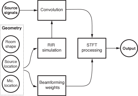
Figure 5: Block diagram of the simulation setup used for numerical experiments.

In this section, we validate the described theoretical results through numerical experiments. First, we analyze the beampatterns produced by the ARR; second, we evaluate the $\mathsf{SINR}$ for various beamformers as a function of the number of image sources used in weight computation; and third, we evaluate the PESQ metric [22]. Finally, we show spectrograms that reveal visually the improved interferer and noise suppression achieved by the ARR.

VI-A Simulation Setup

We use a simple room acoustic framework written in Python, that relies on Numpy and Scipy for matrix computations [27]. We limit ourselves in this paper to 2D geometry and rectangular rooms. In all experiments, the sampling frequency $F_{s}$ was set to 8 kHz. An overview of the simulation setup is shown in Fig. 5.

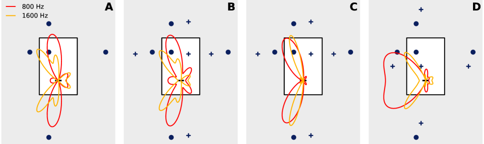
Figure 6: Beam patterns in different scenarios. The rectangular room is 4 by 6 metres and contains a source of interest ($\CIRCLE$) and an interferer (+) ((B), (C), (D) only). The first order image sources are also displayed. The weight computation of the beamformer includes the direct source and the first order image sources of both desired source and interferer (when applicable). (A) Rake-Max-SINR, no interferer, (B) Rake-Max-SINR, one interferer, (C) Rake-Max-UDR, one interferer, (D) Rake-Max-SINR, interferer is in direct path.

Starting from the room geometry and the positions of the sources and microphones, we first compute the locations of all images sources up to ten generations. The reflectivity of the walls is fixed to 0.9. The RIR between the source $\mathbf{s}_{0}$ and the microphone $\mathbf{r}_{m}$ is convolved with an ideal low-pass filter in the continuous domain and then sampled at the sampling frequency $F_{s}$,

$$\widetilde{a}_{m}(\mathbf{s}_{0})[n]=\sum_{k=0}^{K}\frac{\alpha_{k}}{4\pi\|\mathbf{r}_{m}-\mathbf{s}_{k}\|}\,\operatorname{sinc}\left(n-F_{s}\frac{\|\mathbf{r}_{m}-\mathbf{s}_{k}\|}{c}\right),$$ (32)

where $K$ is the number of image sources considered. We choose the limits of $n$ such that the cardinal sine in (32) decays sufficiently to avoid artifacts. The discrete signals from all sound sources are then convolved with their respective RIRs, and added together to obtain the $m$th microphone’s signal.

The beamforming weights are computed in the frequency domain. We use the discrete-time STFT processing with a frame size of $L=4096$ samples, 50% overlap and zero padding on both sides of the signal by $L/2$. A real fast Fourier transform of size $2L$ and a Hann window are used in the analysis. By exploiting the conjugate symmetry of the real FFT we only need to compute $L+1$ beamforming weights, one for every positive frequency bin. The length $L$ is dictated by the length of the beamforming filters in the time-domain and was set empirically to avoid any aliasing in the filter responses. The output signal was synthesized using the conventional overlap-add method [33].

VI-B Results

VI-B1 Beampatterns

We first inspect the beampatterns produced by the Rake-Max-SINR and Rake-Max-UDR beamformers for different source-interferer placements. We consider a $4\text{m}\times 6\text{m}$ rectangular room with a source of interest at $(1\text{m},4.5\text{m})$ and a linear microphone array centered at $(2\text{m},1.5\text{m})$, parallel to the $x$-axis. Spacing between the microphones was set to 8cm. In Fig. 6, we show the beampatterns for four different configurations of the source and the interferer. We consider a scenario without an interferer, one with an interferer placed favorably at $(2.8\text{m},4.3\text{m})$, and finally one where the interferer is placed half-way between the desired source and the array, at $(1.5\text{m},3\text{m})$.

The last scenario is the least favorable. Interestingly, we can observe that the Rake-Max-SINR beampattern adjusts by completely ignoring the direct path, and steering the beam towards the echoes of the source of interest. This is validating the intuition that we can “hear behind an interferer by listening for the echoes”. Note that such a pattern cannot be achieved by a beamformer that only takes into account the direct path. We further note that, while the beampatterns only show the magnitude of the beamformer’s response, the phase plays an important role with multiple sources present.

VI-B2 SINR Gains from Raking

In the experiments in this subsection, we set the power of the desired source and of the interferer to be equal, $\sigma_{x}^{2}=\sigma_{z}^{2}=1$. The noise covariance matrix is set to $10^{-3}\cdot\mathbf{I}_{M}$. We use a circular array of $M=12$ microphones with a diameter of 30 cm, and randomize the position of the desired source and the interferer inside the room. The resulting curves show median performance out of 20000 runs.

Fig. 7 shows output $\mathsf{SINR}$ for different beamformers. The one-forcing beamformer is left out because it performs poorly in terms of $\mathsf{SINR}$, as predicted earlier. Clearly, the Rake-Max-SINR beamformer outperforms all others. The output $\mathsf{SINR}$ for beamformers using only the direct path (Max-SINR and DS) remains approximately constant. The $\mathsf{UDR}$ is plotted against the number of image sources for various beamformers in Fig. 8. The Rake-Max-UDR beamformer performs well in terms of the two measures, its output is perceptually unpleasing due to audible pre-echoes; in informal listening tests, the Rake-Max-SINR beamformer did not produce such artifacts. It is interesting to note that the Rake-Max-SINR also performs well in terms of the $\mathsf{UDR}$. Similar $\mathsf{SINR}$ gains to those in Fig. 7 are observed in Fig. 9 over a range of frequencies. It is therefore justified to extrapolate the results at one frequency in Fig. 7 to the wideband $\mathsf{SINR}$.

VI-B3 Evaluation of Speech Quality

We complement the informal listening tests and the evaluation of $\mathsf{SINR}$ and $\mathsf{UDR}$ with extensive simulations to asses the improvement in speech quality achieved by acoustic raking. We simulate a room with two sources—a desired source and an interferer—and compare the outputs of the Rake-DS, Rake-Max-SINR, and Rake-Max-UDR as a function of the number of image sources used to design the beamformers.

The same number of image sources is used for the target and interferer ($K=K^{\prime}$). The performance metric used is the PESQ [22]. In particular, we use the reference implementation described by the the ITU P.862 Amendment 2 [34]. PESQ compares the reference signal with the degraded signal and predicts the perceptual quality of the latter as it would be measured by the mean opinion score (MOS) value, on a scale from $1$ to $4.5$.

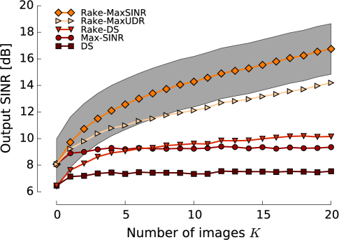
Figure 7: Median output $\mathsf{SINR}$ plotted against the number of image sources used in the design for different beamformers, at a frequency $f=1$ kHz. The shaded area contains the Rake-Max-SINR output $\mathsf{SINR}$s for 50% of the 20000 Monte Carlo runs.

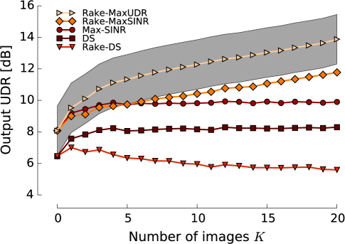
Figure 8: Median output $\mathsf{UDR}$ plotted against the number of image sources used in the design for different beamformers, at a frequency $f=1$ kHz. The shaded area contains the Rake-Max-UDR output $\mathsf{UDR}$s for 50% of the 20000 Monte Carlo runs.

We consider the same room and microphone array setting as before (see Fig. 6A). The desired and the interfering sources are placed uniformly at random in a rectangular area with lower left corner at $(1\text{m},2.5\text{m})$ and upper right corner at $(3\text{m},5\text{m})$. To limit the experimental variation, the speech samples attributed to the sources are fixed throughout the simulation. The two sources start reproducing speech at the same time and approximately overlap for the total duration of the speech samples. The signals are normalized to have the same power at the source. We added white Gaussian noise to the microphone signals, with power chosen so that the $\mathsf{SNR}$ of the direct sound for the desired source is 20 dB at the center of the microphone array. All signals are high-pass filtered with a cut-off frequency of 300 Hz. The reference for all PESQ results is the direct path of the target signal as measured at the center of the array $(2\text{m},1.5\text{m})$.

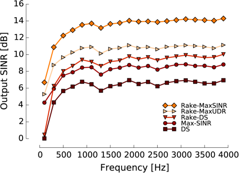
Figure 9: Output $\mathsf{SINR}$ as a function of frequency for different beamformers and $K=K^{\prime}=10$. The curves show the average of 20000 runs, with averaging performed in the dB domain.

The median PESQ measure of 10000 Monte Carlo runs, given in raw MOS, is shown in Fig. 10. The median PESQ of the degraded signal measured at the center of the array before processing was found to be 1.6 raw MOS. When only the direct sound is used (i.e., $K=0$), all three beamformers yield the same improvement of about 0.2 raw MOS. We observe that Rake-DS is marginally better than the other beamformers. Using any number of echoes in addition to the direct sound results in larger MOS for all beamformers. When more than one image source is used, the Rake-Max-SINR beamformer always yields the largest MOS, with up to 0.5 MOS gain when using 10 images sources.

It is worth mentioning that in the beamformer design, we do not assume that we know the spectrum of the source or the interferer—we design as if it was flat. Thus the interferer acts as a strong source of colored, spatially correlated, non-stationary noise, spectrally mismatched with the designed beamformer. There is another source of model mismatch: while the RIRs were computed using hundreds of image sources, we use only up to ten to design the beamformers.

VI-B4 Spectrograms and Sounds Samples

Finally, we present the spectrograms for a scenario where we want to focus on a singer in the presence of interfering speech. We consider the same room, source, interferer, and microphone array geometry as in Fig. 6B.

The source signal is a snippet by a female opera singer (Fig. 11A), with strongly pronounced harmonics; the interfering signal is a male speech extract. The two signals are normalized to have unit maximum amplitude. We add white Gaussian noise to the microphone signals with power such that the SNR of the direct sound of the desired source is 20 dB at the center of the microphone array. All signals are high-pass filtered with a cut-off frequency of 300 Hz. The Rake-Max-SINR beamformer weights are computed using the direct source and three generations of image sources for both the desired sound source (singing) and the interferer (speech).

The output of the conventional Max-SINR beamformer (Fig. 11C) is compared to that of the Rake-Max-SINR (Fig. 11D). We can observe from the spectrogram that the Rake-Max-SINR reduces very effectively the power of the interfering signal at all frequencies, but particularly in the mid to high range. This is true even when the interferer overlaps significantly with the desired signal. Informal listening tests confirm that the Rake-Max-SINR maintains high quality of the desired signal while strongly reducing the interference. The Rake-Max-UDR beamformer provides good interference suppression, but it produces audible pre-echoes that render it unsuitable for speech processing applications. The sound clips can be found online along the code.

VII Conclusion

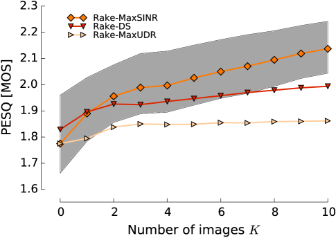
Figure 10: Perceptual quality in MOS, evaluated using PESQ, as a function of the number of image sources used $K$. The lower limit of the ordinates is set to the median MOS of the degraded signal before processing, as measured at center of the array. The shaded area contains the Rake-Max-SINR output for 50% of the 10000 Monte Carlo runs.

We investigated the concept of acoustic rake receivers—beamformers that use echoes. Unlike earlier related work, we presented optimal formulations that outperform the delay-and-sum style approaches by a large margin. This is especially true in the presence of interferers, hence the title “Raking the Cocktail Party”. We demonstrate theoretically that the ARRs improve the $\mathsf{SINR}$, and the numerical simulations agree well with these predictions.

Beyond theoretical and numerical evaluations of the performance measures, we demonstrated in informal listening tests the improved interference suppression by the ARR. Moreover, extensive simulation determined that the ARR improves the subjective quality, as predicted by PESQ, proportionnaly to the number of image sources used. A particularly illustrative example is when the interferer is occluding the desired source—the optimal ARR takes care of this simply by listening to the echoes.

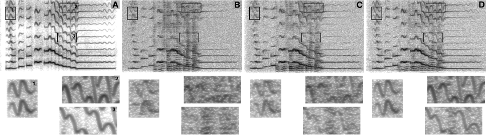
Figure 11: Comparison of the conventional Max-SINR and Rake-Max-SINR beamformer on a real speech sample. Spectrograms of (A) clean signal of interest, (B) signal corrupted by an interferer and additive white Gaussian noise at the microphone input, outputs of (C) conventional Max-SINR and (D) Rake-Max-SINR beamformers. Time naturally goes from left to right, and frequency increases from zero at the bottom up to $F_{s}/2$. To highlight the improvement of Rake-Max-SINR over Max-SINR, we blow-up three parts of the spectrograms in the lower part of the figure. The boxes and the corresponding part of the original spectrogram are numbered in (A). The numbering is the same but omitted in the rest of the figure for clarity.

Perhaps the most important aspect of ongoing work is the design of robust formulations of ARRs. This may involve various heuristics, as well as combinatorial optimization due to the discrete nature of image sources. We expect that the raking beamformers described in this paper inherit the robustness properties of their classical counterparts. For example, the Rake-DS beamformer is likely to be more robust to array calibration errors than the Rake-Max-SINR beamformer. Furthermore, we expect that taking the image source perspective makes various ARRs more robust to errors in source locations than the schemes that assume the knowledge of the RIR.

Another line of ongoing work investigates the time-domain formulations of the ARRs, with some initial results already available [25]. Time-domain formulations offer better control over whether the echoes appear before or after the direct sound. This provides a more natural framework for optimizing perceptually motivated performance measures, such as $\mathsf{UDR}$.

Appendix: Theorem 1

We note that the theorem is is stated for a linear array, but the described behavior is universal.

Theorem 1.

Assume that there are $K+1$ sources located at $\mathbf{s}_{k}=r_{k}[\cos\theta_{k}~{}\sin\theta_{k}]^{T}$ where $\theta_{k}\sim\mathcal{U}(0,2\pi)$ and $r_{k}\sim\mathcal{U}(a,b)$ are all independent, for some $0<a<b$ such that the far-field assumption holds. Let $\mathbf{A}_{s}$ collect the corresponding steering vectors for a uniform linear microphone array. Then $\mathbb{E}\lVert\mathbf{A}_{s}\mathbf{1}\rVert^{2}\geq(1+\beta)\,\mathbb{E}\lVert\mathbf{a}(\mathbf{s}_{0})\rVert^{2}$, where $\beta=\sum_{k=1}^{K}(\alpha_{k}/\alpha_{0})^{2}$, and $\alpha_{k}$ are attenuations of the steering vectors, assumed independent from the source locations. In fact, $\mathbb{E}(\lVert\mathbf{A}_{s}\mathbf{1}\rVert^{2})=(1+\beta)\,\mathbb{E}(\lVert\mathbf{a}(\mathbf{s}_{0})\rVert^{2})+O(1/\Omega^{3})$.

Proof.

Thanks to the far-field assumption, we can decompose the steering vector into a factor due to the array, and a phase factor due to different distances of different image sources. We have that

$$a_{m}=(\mathbf{A}_{s}\mathbf{1})_{m}=\sum_{k=0}^{K}\alpha_{k}\mathrm{e}^{-j{\kappa md\sin\theta_{k}}}\mathrm{e}^{-j{\Omega\delta_{k}/c}},$$ (33)

where $d$ is the microphone spacing and $\kappa\overset{\text{def}}{=}\Omega/c$. Without loss of generality we assume that $\delta_{k}\sim\mathcal{U}(a,b)$. We can further write

$$\mathbb{E}\left|a_{m}\right|^{2} =\mathbb{E}~{}\bigg{[}\bigg{(}\sum_{k=0}^{K}\alpha_{k}\mathrm{e}^{-j{\kappa md\sin\theta_{k}}}\mathrm{e}^{-j{\kappa\delta_{k}}}\bigg{)}$$ (34)

$$\phantom{=\mathbb{E}}\times\bigg{(}\sum_{\ell=0}^{K}\alpha_{\ell}\mathrm{e}^{\hskip 1.0ptj{\kappa md\sin\theta_{\ell}}}\mathrm{e}^{\hskip 1.0ptj{\kappa\delta_{\ell}}}\bigg{)}\bigg{]}$$

$$=\sum_{k=0}^{K}\alpha_{k}^{2}\!+\!\!\!\sum_{k\neq\ell=0}^{K}\!\!\alpha_{k}\alpha_{\ell}\mathbb{E}\left[\mathrm{e}^{\hskip 1.0ptj{\kappa md\left(\sin\theta_{\ell}-\sin\theta_{k}\right)}}\mathrm{e}^{\hskip 1.0ptj{\kappa(\delta_{\ell}-\delta_{k})}}\right].$$

Invoking the independence for $k\neq\ell$, we compute the above expectation as

$$\mathbb{E}\left[\mathrm{e}^{\hskip 1.0ptj{\kappa md\left(\sin\theta_{\ell}-\sin\theta_{k}\right)}}\mathrm{e}^{\hskip 1.0ptj{\kappa(\delta_{\ell}-\delta_{k})}}\right]$$ (35)

$$\hskip 85.35826pt=\frac{2J_{0}^{2}(md\kappa)\big{[}1-\cos(\Delta\kappa)\big{]}}{(\Delta\kappa)^{2}},$$

where $J_{0}$ denotes the Bessel function of the first kind and zeroth order and $\Delta\overset{\text{def}}{=}b-a$.

Plugging this back into (34), we obtain

$$\mathbb{E}\left|a_{m}\right|^{2}=\sum_{k=0}^{K}\alpha_{k}^{2}\left(1+C\frac{2J_{0}^{2}(md\kappa)\big{[}1-\cos(\Delta\kappa)\big{]}}{(\Delta\kappa)^{2}}\right),$$ (36)

where $C=\sum_{k\neq\ell}\alpha_{k}\alpha_{\ell}/\sum_{k}\alpha_{k}^{2}$.

Because $\left|J_{0}(z)\right|\leq\sqrt{2/(\pi z)}+O(\left|z\right|^{-1})$ ([35], Eq. 9.2.1), we see that the expression in brackets is $1+O(\Omega^{-3})$. Rewriting

$$\sum_{k=0}^{K}\alpha_{k}^{2}=\frac{1}{M}\mathbb{E}\lVert\mathbf{a}(\mathbf{s}_{0})\rVert^{2}\left(1+\sum_{k=1}^{K}(\alpha_{k}/\alpha_{0})^{2}\right)$$ (37)

concludes the proof. ∎

References

- [1] R. Price and P. E. Green, “A Communication Technique for Multipath Channels,” in Proceedings of the IRE. 1958, pp. 555–570, IEEE.
- [2] A. F. Naguib, “Space-time receivers for CDMA multipath signals,” in Proc. IEEE ICC, Montreal, 1997, pp. 304–308, IEEE.
- [3] B. H. Khalaj, A. Paulraj, and T. Kailath, “2D RAKE Receivers for CDMA Cellular Systems,” in Proc. IEEE GLOBECOM. 1994, pp. 400–404, IEEE.
- [4] P. Annibale, F. Antonacci, P. Bestagini, A. Brutti, A. Canclini, L. Cristoforetti, J. Filos, E. Habets, W. Kellerman, K. Kowalczyk, A. Lombard, E. Mabande, D. Markovic, P. Naylor, and M. Omologo, “The SCENIC Project: Space-Time Audio Processing for Environment-Aware Acoustic Sensing and Rendering,” in 131st Convention of the Audio Engineering Society, New York, NY, USA, 2011, Audio Engineering Society.
- [5] A. E. O’Donovan, R. Duraiswami, and D. N. Zotkin, “Automatic Matched Filter Recovery via the Audio Camera,” in Proc. IEEE ICASSP, Dallas, 2010, pp. 2826–2829, IEEE.
- [6] E.-E. Jan, P. Svaizer, and J. L. Flanagan, “Matched-Filter Processing of Microphone Array for Spatial Volume Selectivity,” Proc. IEEE ISCAS, vol. 2, pp. 1460–1463, 1995.
- [7] J. B. Allen and D. A. Berkley, “Image Method For Efficiently Simulating Small-room Acoustics,” J. Acoust. Soc. Am., vol. 65, no. 4, pp. 943–950, 1979.
- [8] J. Borish, “Extension of the Image Model To Arbitrary Polyhedra,” J. Acoust. Soc. Am., vol. 75, no. 6, pp. 1827–1836, 1984.
- [9] D. B. Ward, E. A. Lehmann, R. C. S. Williamson, and A. P. I. T. on, “Particle Filtering Algorithms for Tracking an Acoustic Source in a Reverberant Environment,” IEEE Trans. Audio, Speech, Language Process., vol. 11, no. 6, pp. 826–836, 2003.
- [10] F. Ribeiro, D. A. Florencio, D. E. Ba, and C. Zhang, “Geometrically Constrained Room Modeling With Compact Microphone Arrays,” IEEE Trans. Acoust., Speech, Signal Process., vol. 20, no. 5, pp. 1449–1460, 2012.
- [11] F. Antonacci, J. Filos, M. R. P. Thomas, E. A. P. Habets, A. Sarti, P. A. Naylor, and S. Tubaro, “Inference of Room Geometry From Acoustic Impulse Responses,” IEEE Trans. Acoust., Speech, Signal Process., vol. 20, no. 10, pp. 2683–2695, 2012.
- [12] I. Dokmanic, Y. M. Lu, and M. Vetterli, “Can One Hear the Shape of a Room: The 2-D Polygonal Case,” in Proc. IEEE ICASSP, Prague, 2011, pp. 321–324.
- [13] I. Dokmanić, R. Parhizkar, A. Walther, Y. M. Lu, and M. Vetterli, “Acoustic echoes reveal room shape,” Proc. Natl. Acad. Sci., vol. 110, no. 30, June 2013.
- [14] J. S. Bradley, H. Sato, and M. Picard, “On the Importance of Early Reflections for Speech in Rooms,” J. Acoust. Soc. Am., vol. 113, no. 6, pp. 3233, 2003.
- [15] J. Lochner and J. F. Burger, “The Influence of Reflections on Auditorium Acoustics,” J. Sound Vib., vol. 1, no. 4, pp. 426–454, 1964.
- [16] E. Habets, J. Benesty, I. Cohen, S. Gannot, and J. Dmochowski, “New Insights Into the MVDR Beamformer in Room Acoustics,” IEEE Trans. Audio, Speech, Language Process., vol. 18, no. 1, pp. 158–170, Jan. 2010.
- [17] M. R. P. Thomas, N. D. Gaubitch, and P. A. Naylor, “Application of Channel Shortening to Acoustic Channel Equalization in the Presence of Noise and Estimation Error,” in Proc. IEEE WASPAA, New Paltz, NY, 2011, pp. 113–116, IEEE.
- [18] W. Zhang, E. Habets, and P. A. Naylor, “On the Use of Channel Shortening in Multichannel Acoustic System Equalization,” in Proc. IWAENC, Tel Aviv, 2010.
- [19] M. Miyoshi and Y. Kaneda, “Inverse Filtering of Room Acoustics,” IEEE Trans. Acoust., Speech, Signal Process., vol. 36, no. 2, pp. 145–152, 1988.
- [20] K. Furuya, “Noise Reduction and Dereverberation using Correlation Matrix Based on the Multiple-Input/Output Inverse-Filtering Theorem (MINT),” in Proc. Intl. Workshop on HSC, Kyoto, Japan, 2001, pp. 59–62.
- [21] J. Benesty, J. Chen, Y. A. Huang, and J. Dmochowski, “On Microphone-Array Beamforming From a MIMO Acoustic Signal Processing Perspective,” IEEE Trans., Audio, Speech, Language Process., vol. 15, no. 3, pp. 1053–1065, Mar. 2007.
- [22] A. W. Rix, J. G. Beerends, M. P. Hollier, and A. P. Hekstra, “Perceptual Evaluation of Speech Quality (PESQ)—A New Method for Speech Quality Assessment of Telephone Networks and Codecs,” in Proc. IEEE ICASSP, Salt Lake City, UT, 2001, pp. 749–752.
- [23] S. Haykin and Z. Chen, “The Cocktail Party Problem,” Neural Comput., vol. 17, no. 9, pp. 1875–1902, 2005.
- [24] W. Herbordt and W. Kellermann, “Adaptive Beamforming for Audio Signal Acquisition,” in Adaptive Signal Processing, pp. 155–194. Springer, Berlin, Heidelberg, Feb. 2003.
- [25] R. Scheibler, I. Dokmanić, R, and M. Vetterli, “Raking Echoes in the Time Domain,” Accepted to IEEE ICASSP, 2015.
- [26] B. D. Carlson, “Covariance Matrix Estimation Errors and Diagonal Loading in Adaptive Arrays,” IEEE Trans. Aerosp. Electron. Syst., vol. 24, no. 4, pp. 397–401, July 1988.
- [27] T. E. Oliphant, “Python for Scientific Computing,” Computing in Science & Engineering, vol. 9, no. 3, pp. 10–20, 2007.
- [28] D. Duffy, Green’s Functions with Applications, Chapman and Hall/CRC, 2001.
- [29] B. D. Van Veen and K. M. Buckley, “Beamforming: A Versatile Approach to Spatial Filtering,” IEEE ASSP Mag., vol. 5, no. 2, pp. 4–24, 1988.
- [30] O. L. I. Frost, “An Algorithm for Linearly Constrained Adaptive Array Processing,” in Proc. IEEE. 1972, pp. 926–935, IEEE.
- [31] W. McCrea and F. Whipple, “Random Paths in Two and Three Dimensions,” in Proc. Roy. Soc. Edinburgh, 1940, vol. 60, pp. 281–298.
- [32] O. Öçal, I. Dokmanić, and M. Vetterli, “Source Localization and Tracking in Non-Convex Rooms,” Proc. IEEE ICASSP, 2014.
- [33] J. J. Shynk, “Frequency-Domain and Multirate Adaptive Filtering,” IEEE Signal Process. Mag., vol. 9, no. 1, pp. 14–37, 1992.
- [34] ITU-T P.862 Amendment 2, “Reference Implementations and Conformance Testing for ITU-T Recs P.862, P.862.1 and P.862.2,” 11 2005.
- [35] M. Abramowitz and I. A. Stegun, Handbook of Mathematical Functions, Courier Dover Publications, 1972.