WASP 1628+10 – an EL CVn-type binary with a very-low-mass stripped-red-giant star and multi-periodic pulsations.

Abstract

The star 1SWASP J162842.31+101416.7 (WASP 1628+10) is one of several EL CVn-type stars recently identified using the WASP database, i.e., an eclipsing binary star in which an A-type dwarf star (WASP 1628+10 A) eclipses the remnant of a disrupted red giant star (WASP 1628+10 B). We have measured the masses, radii and luminosities of the stars in WASP 1628+10 using photometry obtained in three bands (u’, g’, r’) with the Ultracam instrument and medium-resolution spectroscopy. The properties of the remnant are well-matched by models for stars in a rarely-observed state evolving to higher effective temperatures at nearly constant luminosity prior to becoming a very low-mass white dwarf composed almost entirely of helium, i.e., we confirm that WASP 1628+10 B is a pre-He-WD. WASP 1628+10 A appears to be a normal A2 V star with a mass of $1.36\pm 0.05$${M}_{\sun}$. By fitting models to the spectrum of this star around the H$\gamma$ line we find that it has an effective temperature ${\rm T}_{\rm eff,A}=7500\pm 200$ K and a metallicity $[{\rm Fe/H}]=-0.3\pm 0.3$. The mass of WASP 1628+10 B is only $0.135\pm 0.02$${M}_{\sun}$. The effective temperature of this pre-He-WD is approximately 9200 K. The Ultracam photometry of WASP 1628+10 shows variability at several frequencies around 40 cycles per day, which is typical for $\delta$ Sct-type pulsations often observed in early A-type stars like WASP 1628+10 A. We also observe frequencies near 114 cycles/day and 129 cycles/day, much higher than the frequencies normally seen in $\delta$ Sct stars. Additional photometry through the primary eclipse will be required to confirm that these higher frequencies are due to pulsations in WASP 1628+10 B. If confirmed, this would be only the second known example of a pre-He-WD showing high-frequency pulsations.

1 Introduction

1SWASP J162842.31+101416.7 (WASP 1628+10 hereafter) is one of several million bright stars ($8\la V\la 13$) that have been observed by the Wide Angle Search for Planets, (WASP, Pollacco et al. 2006). Maxted et al. (2014) showed that this star is an eclipsing binary star with an orbital period of 0.72 days that contains an A-type dwarf star (WASP 1628+10 A) and the precursor of a helium white dwarf (pre-He-WD) with a mass $\la 0.3\mbox{${M}_{\sun}$}$ (WASP 1628+10 B).

Low-mass white dwarf stars ($M\la 0.35\mbox{${M}_{\sun}$}$) are the product of binary star evolution (Iben & Livio, 1993; Marsh et al., 1995). Various evolution channels exist, but they are generally the result of mass transfer from an evolved main sequence star or red giant star onto a companion star. Towards the end of the mass transfer phase the donor star will have a degenerate helium core. This “stripped red giant star” does not have sufficient mass to ignite helium, and so the white dwarf that emerges has an anomalously low mass and is composed almost entirely of helium. For this reason, they are known as helium white dwarfs (He-WDs). If the companion to the red giant is a neutron star then the mass transfer is likely to be stable so the binary can go on to become a low mass X-ray binary containing a millisecond pulsar. Several millisecond radio pulsars are observed to have low-mass white dwarf companions (Lorimer, 2008). Many He-WDs have been identified in the Sloan Digital Sky Survey (Kilic et al., 2007), some with masses as low as 0.16${M}_{\sun}$ (Kilic et al., 2012), and from proper motion surveys (Kawka & Vennes, 2009). Helium white dwarfs can also be produced by mass transfer from a red giant onto a main sequence star, either rapidly through unstable common-envelope evolution or after a longer-lived “Algol” phase of stable mass transfer (Refsdal & Weigert, 1969; Giannone & Giannuzzi, 1970; Willems & Kolb, 2004; Iben & Livio, 1993; Chen & Han, 2003; Nelson & Eggleton, 2001). He-WDs may also be the result of collisions in dense stellar environments such as the cores of globular clusters (Knigge et al., 2008), or by tidal stripping of a red giant star by a super-massive black hole (Bogdanovic et al., 2013).

The evolution of He-WDs is expected to be very different from more massive white dwarfs. If the time scale for mass loss from the red giant is longer than the thermal timescale, then when mass transfer ends there will still be a thick layer of hydrogen surrounding the degenerate helium core. The mass of the hydrogen layer depends on the total mass and composition of the star (Nelson et al., 2004), but is typically 0.001 – 0.005${M}_{\sun}$, much greater than for typical white dwarfs (hydrogen layer mass $<10^{-4}$${M}_{\sun}$). The pre-He-WD then evolves at nearly constant luminosity towards higher effective temperatures while the hydrogen layer mass is gradually reduced by stable shell burning of hydrogen via the CNO cycle. This pre-He-WD phase can last several million years for lower mass stars with thicker hydrogen envelopes. CNO fusion becomes less efficient towards the end of this phase so the star starts to fade and cool.

The smooth transition from a pre-He-WD to a He-WD can be interrupted by one or more phases of unstable CNO burning (shell flashes) for pre-He-WDs with masses $\approx 0.2$ – 0.3${M}_{\sun}$ (Webbink, 1975; Driebe et al., 1999). These shell flashes substantially reduce the mass of hydrogen that remains on the surface. The mass range within which shell flashes are predicted to occur depends on the assumed composition of the star and other details of the models (Althaus et al., 2001). The cooling timescale for He-WDs that do not undergo shell flashes is much longer than for those that do because their thick hydrogen envelopes can support residual p-p chain fusion for several billion years.

Maxted et al. (2013) presented strong observational support for the assumption that He-WDs are born with thick hydrogen envelopes. They found that only models with thick hydrogen envelopes could simultaneously match their precise mass and radius estimates for both stars in the EL CVn-type binary WASP 0247$-$25, together with other observational constraints such as the orbital period and the likely composition of the stars based on their kinematics. In addition, they found that the pre-He-WD WASP 0247$-$25 B is a new type of variable star in which a mixture of radial and non-radial pulsations produce multiple frequencies in the lightcurve near 250 cycles/day. This opens up the prospect of using asteroseismology to study the interior of this star, e.g., to measure its internal rotation profile.

In this paper we present new spectroscopy of WASP 1628+10 that we use to confirm that WASP 1628+10 B is a pre-He-WD and new photometry that suggests this pre-He-WD also shows pulsations at more than one frequency.

2 Observations

2.1 Spectroscopy

We obtained 41 spectra of WASP 1628+10 on the nights 2013 May 20 – 24 using the Intermediate Dispersion Spectrograph (IDS) on 2.5-m Isaac Newton Telescope at the Observatorio del Roque de los Muchachos on La Palma, Spain. We used the H2400B grating and a 1.2 arcsecond slit with the EEV10 charge coupled device (CCD) detector to obtain spectra with a dispersion of 0.23Å/pixel at 4350Å. The resolution of the spectra estimated by fitting the several lines in a calibration arc spectrum is 0.45Å. The unvignetted portion of the CCD covers the wavelength range 4115 – 4635Å. Spectra were extracted using the optimal extraction algorithm of Horne (1986) in the pamela application distributed by the Starlink project. Observations of each star were bracketed with arc spectra and the wavelength calibration established from these arcs interpolated to the time of mid-exposure. The exposure times used were 600 s or 900 s, resulting in spectra with a typical signal-to-noise ratio of 25 – 45 per pixel. The spectra were flux calibrated using a spectrum of the star BD+28 4211 (Oke, 1990) obtained using a wide slit.

2.2 Photometry

We obtained photometry of WASP 1628+10 using the multi-channel photometer Ultracam (Dhillon et al., 2007) mounted on the William Herschel 4.2-m telescope at the Observatorio del Roque de los Muchachos. Images of WASP 1628+10 and the comparison star TYC 964-558-1 were obtained simultaneously through u’, g’ and r’ filters with an exposure time of 0.55 seconds for the g’ and r’ images and 1.65 seconds for the u’ images. Ultracam is a frame-transfer device and we only read-out the data in windows around the target and comparision star so the dead-time between the exposures in only 25 ms. The image scale is 0.3 arcseconds per pixel. A log of the observations is provided in Table 1.

Table 1: Observing log for our Ultracam observations of WASP 1628+10. “Night” is the UTC date at the start of the night.

Night	Start	End	Notes
(UTC)	(UTC)	(UTC)
2013 04 21	03:13	06:08	Secondary eclipse
2013 04 22	00:09	06:01
2013 04 23	23:09	00:57	Primary eclipse
2013 04 23	03:04	05:59
2013 04 24	23:12	01:24

All reductions were performed with the Ultracam pipeline software. The images were bias-subtracted and flat-fielded using twilight sky exposures in the normal way. We used synthetic aperture photometry to measure the apparent flux of WASP 1628+10 and the comparison star. The aperture radius was set to twice the full-width at half-maximum (FWHM) of the stellar profile in each image. The FWHM of the stellar profile was typically 1.5 – 2 arcsec.

3 Analysis

3.1 Photometry

3.1.1 Pulsations

We used the period04 software package (Lenz & Breger, 2005) to search for periodic variations in the three Ultracam datasets listed in Table 1 that do not include an eclipse. For each dataset we first removed data affected by clouds and then divided the differential magnitudes by a low-order polynomial fit by least-squares. Periodograms were generated for the u’, g’ and r’ data independently over the frequency range 0 – 1000 cycles/day in 0.017 cycle/day steps using the flux values in 10 s bins weighted by the standard error of the mean in each bin. The resulting periodograms are shown in Fig. 1. We identified the frequency with the highest peak in this periodogram and then performed a least-squares fit to the data to optimise the values of the amplitude, phase and frequency of this signal. We then identified the strongest frequency in the periodogram using the residuals from this fit, and performed another least squares fit to optimise all the frequencies, phases and amplitudes. This process was repeated until we judged that the strongest frequency detected in the residuals was due to noise. The frequencies detected in each dataset and their amplitudes are listed in Table 2.

The comparision star we used has optical-infrared magnitudes entirely consistent with those of a typical mid-K-type star. The other stars in the Ultracam field of view are too faint to be useful as comparison stars. The WASP lightcurve of the comparision star star has over 30,000 observations over 5 years and is constant to with 0.02 magnitudes. There is no reason to expect that such a star would show variability at the amplitudes and frequencies seen in our Ultracam data.

Some of the power at low frequencies ($\la 20$ cycles/day) in these data may be due to offsets between data from different nights. The poor sampling of the data also means that there are problems with 1-day aliases of real periodic signals in the periodograms. Nevertheless, there are three frequencies seen in the u’, g’ and r’ data sets that agree to better than 0.5 per cent. These are indicated in Fig. 1 and the mean value of these frequencies with their standard errors are given in Table 2. There are clearly other frequencies in the range 25 – 50 cycles/day present in the data, but we are unable to reliably identify the correct alias from the data currently available.

Table 2: Frequencies detected in our Ultracam data of WASP 1628+10. Amplitudes are given as the semi-amplitude of the fractional flux variation. The standard error in the final digit of the mean value is given in parentheses. The values listed here are the result of a least-squares fit to the data to optimise the frequency, phase and amplitudes of all the frequencies listed.

Frequency (cycles/day)				Amplitude ($/10^{-3}$)
u’	g’	r’	Mean		u’	g’	r’
15.38	13.71				0.6	0.8
32.49	27.40	25.13			1.0	0.6	0.5
37.86	28.82	31.51			0.9	1.1	0.8
	36.85	41.84				1.0	0.7
42.13	42.11	42.20	42.15(3)		2.4	2.3	1.7
44.36	43.53				1.0	1.2
114.4	114.4	114.4	114.40(1)		1.3	0.7	0.4
129.2	129.2	129.2	129.23(1)		0.9	0.5	0.4

Figure 1: Periodograms of the out-of-eclipse Ultracam data of WASP 1628+10. The three frequencies detected in all three channels are indicated.

3.1.2 Eclipses

Our Ultracam observations include the ingress to one secondary eclipse and observations of one primary eclipse with gaps due to thin cloud. We used jktebop version 28 (Southworth 2010 and references therein) to analyse the data from the u’, g’ and r’ bands independently using the ebop lightcurve model (Etzel, 1981; Popper & Etzel, 1981). We used the feature available in jktebop to modulate the flux from either star using up to 5 sinusoidal functions, $A_{i}\sin[2\pi(t-T_{i})f_{i}]$. We included in our lightcurve model sinusoids at the 3 frequencies listed in Table 2 detected in all three channels plus the 2 other sinusoids at the frequencies with the largest amplitudes in each channel. The phase and amplitude of each frequency were included as free parameters in the fit. We assumed that frequencies $>100$ cycles/day originate from WASP 1628+10 B and that lower frequencies originate from WASP 1628+10 A. There is little difference to the quality of the fit or the parameters derived if all the frequencies are assigned to WASP 1628+10 A. We used magnitude values in 10 s bins with equal weight for each binned data point for the least-squares fit. Other free parameters in the least-squares fit were: a normalisation constant, the surface brightness ratio $J=S_{B}/S_{A}$, where $S_{A}$ is the surface brightness of WASP 1628+10 A and similarly for $S_{B}$; the sum of the radii relative to semi-major axis, $s=(R_{\rm A}+R_{\rm B})/a$; the ratio of the radii, $k=R_{\rm B}/R_{\rm A}$; the orbital inclination, $i$; the phase of primary eclipse, $\Delta$. The orbital phase of the observations was calculated using the ephemeris for the time of primary eclipse (min I) derived from a similar lightcurve fit to the WASP photometry of WASP 1628+10 by Maxted et al. (2014), which we quote here for convenience:

$${\rm HJD(UTC)~{}min~{}I}=2454921.8532(5)+0.7203633(9)\times E.$$

The standard errors on the final digits quoted in parantheses imply a standard error in the phase of the Ultracam observations of 0.0025. The mass ratio was fixed at the value derived from the spectroscopy described below. Linear limb-darkening coefficients for star A were taken from Claret (2004). We assumed that the orbit is circular and fixed the gravity darkening coefficients of both stars to 0.5 since this parameter has a negligible effect on the shape of the eclipses. The linear limb darkening coefficient of star B also has a negligible effect on the lightcurve so was fixed at a value of 0.5. The results are given in Table 3. The observed lightcurves and the model fits are shown in Fig. 2.

It is difficult to assign reliable error estimates to the parameters derived from the individual lightcurves because of the large number of possible pulsation frequencies that may be present in the data and the unknown effect of the pulsations on the shape of the ingress and egress to the eclipses (Bíró & Nuspl, 2011). Instead, we simply quote the values derived from each lightcurve plus the values derived by Maxted et al. (2014) for the same parameters using the WASP photometry and an r’ lightcurve obtained with the PIRATE telescope. We then adopt the mean values of the parameters that do not depend on wavelength from these 5 lightcurve fits and use the standard error on the mean to estimate the standard errors for these estimates. These mean values and their standard errors are also given in Table 3.

Table 3: Parameters for the lightcurve models fit by least-squares. Parameters fixed in the least-squares fit are preceeded by “=”. The luminosity ratio in each band is $\ell=L_{B}/L_{A}$, other parameter definitions are given in the text. $N$ is the number of points used in the least-squares fit and RMS is the standard deviation of the residuals. Results for the fits to the PIRATE r’ and WASP lightcurves are from Maxted et al. (2014). HMJD is heliocentric modified Julian date.

			Ultracam			PIRATE	WASP
Parameter		Units	u’	g’	r’	r’	–	Mean
$J$	Surface brightness ratio		$2.23$	$1.74$	$1.79$	$1.90$	$1.79$	$J_{\rm r^{\prime}}=1.85\pm 0.06$
$s$	Sum of fractional radii		$0.495$	$0.508$	$0.499$	$0.491$	$0.488$	$0.496\pm 0.004$
$k$	Ratio of the radii		$0.225$	$0.230$	$0.215$	$0.209$	$0.227$	$0.221\pm 0.004$
$u_{A}$	Linear limb darkening coefficient		$=0.72$	$=0.68$	$=0.54$	$0.31$	$0.84$
$i$	Orbital inclination	∘	$73.4$	$73.3$	$72.4$	$72.9$	$73.7$	$73.1\pm 0.2$
$\Delta$	Phase offset of primary eclipse		$0.0036$	$0.0053$	$0.0024$			$0.0038\pm 0.0008$
$\ell$	Luminosity ratio		$0.137$	$0.109$	$0.087$	$0.083$	$0.094$	$\ell_{\rm r^{\prime}}=0.085\pm 0.002$
$R_{A}/a$	Fractional radius of star A		$0.404$	$0.412$	$0.411$	$0.406$	$0.398$	$0.406\pm 0.003$
$R_{B}/a$	Fractional radius of star B		$0.091$	$0.095$	$0.089$	$0.085$	$0.090$	$0.090\pm 0.002$
$f_{1}$		d-1	$=42.15$	$=42.15$	$=42.15$
$T_{1}$		HMJD	$0.0036$	$0.0009$	$0.0009$
$A_{1}$		mmag	$-2.1$	$-2.5$	$-1.2$
$f_{2}$		d-1	$=114.40$	$=114.40$	$=114.40$
$T_{2}$		HMJD	$-0.0004$	$-0.0012$	$-0.0010$
$A_{2}$		mmag	$12.8$	$12.4$	$8.6$
$f_{3}$		d-1	$=129.23$	$=123.23$	$=123.23$
$T_{3}$		HMJD	$-0.0046$	$-0.0004$	$-0.0003$
$A_{3}$		mmag	$5.3$	$-6.0$	$-4.1$
$f_{4}$		d-1	$=32.49$	$=43.53$	$=31.51$
$T_{4}$		HMJD	$-0.0228$	$-0.0001$	$0.2287$
$A_{4}$		mmag	$-1.4$	$2.1$	$0.9$
$f_{5}$		d-1	$=37.86$	$=28.82$	$=41.84$
$T_{5}$		HMJD	$-0.0016$	$0.0417$	$-0.0189$
$A_{5}$		mmag	$-2.8$	$1.2$	$-1.2$
N			$3052$	$3094$	$3063$	$480$	$30131$
RMS		mmag	$9.2$	$3.8$	$3.4$	$6$	$42$

Figure 2: From bottom-to-top: Ultracam u’, g’ and r’ lightcurves of the primary and secondary eclipses of WASP 1628+10 (points) with our least-squares fits to these data (lines). Note that the model fits shown do not include the modulation of the signal due to pulsations.

3.2 Spectroscopy

3.2.1 Radial velocity measurements

We first attempted to measure the radial velocities of WASP 1628+10 A using cross-correlation against the spectrum of $\theta$ Leo, an A2 V-type star with narrow lines, obtained with the same instrumental setup. We excluded the broad H$\gamma$ line from the calculation of the cross-correlation functions (CCFs) and measured the radial velocity from a parabolic fit to the three highest points in the CCF. The resulting radial velocities show large scatter and obvious offsets between spectra obtained at the same orbital phase on different nights. We assume that these systematic errors are the result of $\delta$ Scuti-type pulsations in WASP 1628+10 A. These pulsations will cause distortions of the spectral lines (e.g., Kennelly et al., 1998). Some evidence for this is provided by the observation that the measured radial velocities show better agreement from night-to-night if we apply a Gaussian smoothing algorithm to the template spectrum. This is presumably a result of the broader line profiles in a broadened template being less sensitive to the detailed shape of distorted line profiles. To derive the semi-amplitude, $K_{\rm A}$, from these radial velocities we use a least-squares fit of a circular orbit, i.e., the function $V_{r}=\gamma_{\rm A}+K_{\rm A}\sin[2\pi(t-T_{0})/P]$ with $\gamma_{\rm A}$ and $K_{\rm A}$ as free parameters and $T_{0}$ and $P$ fixed at the values given in Section 3.1.2. This gives a good fit to the radial velocities measured with a smoothed template spectrum, but the derived value of the velocity semi-amplitude then shows a dependence on the width of the Gaussian smoothing kernel used.

We also measured the radial velocity of WASP 1628+10 A using a best-fit synthetic spectrum derived from the analysis described in section 3.3.1. We found that the radial velocities derived varied systematically depending on the method used to measure the position of the CCF, e.g., a parabolic fit to the highest three points leads to a value of $K_{A}$ lower by about 2.5${\mathrm{km}\,\mathrm{s}}^{-1}$ than the value derived from a Gaussian profile fit to the region $\pm 100$ ${\mathrm{km}\,\mathrm{s}}^{-1}$ around the peak of the CCF. The radial velocities measured using this latter method are given in Table 4 and the least-squares fit of a circular orbit to these velocities is shown in Fig. 3.

For this analysis we adopt the values $\gamma_{\rm A}=-39\pm 3$ ${\mathrm{km}\,\mathrm{s}}^{-1}$ and $K_{\rm A}=24\pm 3$ ${\mathrm{km}\,\mathrm{s}}^{-1}$, where the adopted values are from the least-squares fit the the radial velocities given in Table 4 and the estimated standard errors reflect the range of different values derived from different methods for measuring the radial velocity.

Table 4: Measured radial velocities of WASP 1628+10 A. These measurements are affected by systematic errors due to pulsations and so we do not quote the standard errors derived from the fitting procedure here.

HJD(UTC)	$V_{r}$	HJD(UTC)	$V_{r}$
$-2\,450\,000$	[${\mathrm{km}\,\mathrm{s}}^{-1}$]	$-2\,450\,000$	[${\mathrm{km}\,\mathrm{s}}^{-1}$]
6433.4478	$13.4$	6435.4758	$21.7$
6433.4549	$12.8$	6435.4863	$28.2$
6433.4620	$13.8$	6435.5274	$22.3$
6433.6060	$-8.0$	6435.5380	$26.3$
6433.6165	$-15.0$	6435.5485	$26.3$
6433.6270	$-13.9$	6435.5602	$27.2$
6434.4620	$-23.9$	6435.5707	$25.8$
6434.4690	$-17.3$	6435.5813	$22.0$
6434.4761	$-22.9$	6436.5153	$-15.6$
6434.5070	$-21.0$	6436.5258	$-16.7$
6434.5141	$-15.8$	6436.5363	$-20.8$
6434.5212	$-15.1$	6436.5480	$-20.6$
6434.5326	$-17.3$	6436.5585	$-21.6$
6434.5986	$-3.6$	6436.5690	$-22.7$
6434.6057	$-1.4$	6436.5807	$-19.2$
6434.6128	$0.4$	6436.5912	$-21.0$
6434.6198	$4.3$	6436.6018	$-19.3$
6434.6269	$2.9$	6436.6591	$-18.1$
6434.7146	$17.7$	6436.6696	$-18.8$
6434.7217	$22.2$	6436.6802	$-17.0$
6434.7287	$18.9$

To measure the radial velocity of WASP 1628+10 B, we first subtracted a scaled and shifted version of a best-fit synthetic spectrum of WASP 1628+10 A from all the spectra observed between orbital phases 0.1 and 0.9. This removes almost all of the signal of WASP 1628+10 A from these spectra, revealing the spectrum of WASP 1628+10 B (Fig. 4). Some weak features from the spectrum of WASP 1628+10 A remain in these spectra because of the line profile variations caused by the pulsations in this star. The Mg II 4481Å line from WASP 1628+10 B can be clearly seen in these spectra, but is difficult to measure in individual spectra. Instead, we simultaneously fit a Gaussian profile to all these spectra with the position of the line in the spectrum observed at time $t$ set by a radial velocity offset $\gamma_{\rm B}+K_{\rm B}\sin(2\pi(t-T_{0})/P)$. The width and depth of the line are also free parameters in the least-squares fit. With this method we obtain the values $\gamma_{\rm B}=-41\pm 2$ ${\mathrm{km}\,\mathrm{s}}^{-1}$ and $K_{\rm B}=-236\pm 3$ ${\mathrm{km}\,\mathrm{s}}^{-1}$. The value of $\gamma_{\rm B}$ agrees well with the value of $\gamma_{\rm A}$ derived from the radial velocities of WASP 1628+10 A.

Figure 3: Radial velocities of WASP 1628+10 A, measured using cross-correlation against a synthetic template spectrum generated by SME for the parameters T_eff=7500 K, $\log\,{\mathrm{g}}$=4.2, ${\mathrm{V}}_{\mathrm{rot}}\sin i$=105${\mathrm{km}\,\mathrm{s}}^{-1}$. The solid line is a circular orbit with the parameters $K_{\rm A}=23$${\mathrm{km}\,\mathrm{s}}^{-1}$ and the dotted line indicates the mean radial velocity $\gamma=-39$${\mathrm{km}\,\mathrm{s}}^{-1}$.

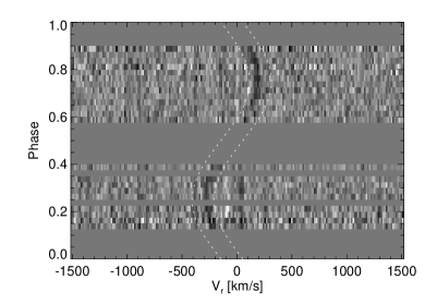
Figure 4: Grey-scale plot showing spectra of WASP 1628+10 after subtraction of a synthetic spectrum for WASP 1628+10 A. The sinusoidal signal highlighted with dotted lines is the Mg II 4481 line from WASP 1628+10 B. The absorption and emission features near 0 ${\mathrm{km}\,\mathrm{s}}^{-1}$ are residuals from the spectral subtraction due to line profile variations in WASP 1628+10 A.

3.2.2 Disentangled spectra

Disentangling refers to the recovery of the individual spectra of two stars from a series of combined spectra in which the individual spectra have different radial velocity shifts due to the orbital motion in the binary system. Here we use our own implementation of the algorithm by Simon & Sturm (1994) that uses a sparse matrix inversion technique to recover the individual spectra. In outline, the problem we wish to solve is to find the matrix $x$ that solves the equation $A\cdot x=b$ in the least-squares sense, where $b$ is a column vector containing the observed spectra, $x$ are the two individual spectra and $A$ performs a linear interpolation of $x$ onto $b$ accounting for the known radial velocity shifts of the two stars. We have modified this algorithm to account for the fact that some of our spectra were observed during the total eclipse of WASP 1628+10 B. This is advantageous because it removes the ambiguity over the contribution of each star to the combined continuum level. The modification is straightforward since it only requires the matrix elements of $A$ to by multiplied by the fractional contribution of each star to the combined spectrum, i.e., $0$ in the case of the matrix elements corresponding to WASP 1628+10 B observed during the primary eclipse. To find the optimum luminosity ratio of the two stars in the spectra observed outside of eclipse, $\ell$, we calculated the standard deviation of the residuals ($\sigma$) over a grid of $\ell$ values, and then interpolated to the value of $\ell=0.132$ that minimizes $\sigma$. This value is in good agreement with the value of $\ell$ we would expect based on the fits to the u’- and g’-band lightcurves (Table 3).

3.3 Effective temperature estimates

3.3.1 SME fits to the disentangled spectra

We have used the software package sme (“Spectroscopy Made Easy”, Valenti & Piskunov, 1996) version 412 beta to fit synthetic spectra based on Kurucz’ atlas9 model atmospheres (Heiter et al., 2002) to the disentangled spectra of WASP 1628+10 A and WASP 1628+10 B. Atomic and molecular line data were obtained from the Vienna Atomic Line Database version VALD3. The option to use the extended treatment of van der Waals broadening was used (Barklem et al., 1998). Line lists for each star were generated using the “Extract Stellar” option of VALD3 to find lines with an expected depth of at least 0.01 for stars with $\mbox{T${}_{\mathrm{eff}}$}=7500$ K or $\mbox{T${}_{\mathrm{eff}}$}=8500$ K, $\log g=4.5$ and solar composition. We fitted the entire available spectral range, which includes the red wing of the H$\delta$ line and the entire H$\gamma$ line. The free parameters in the fit were the radial velocity, $V_{r}$; the projected equatorial rotational velocity, ${\mathrm{V}}_{\mathrm{rot}}\sin i$; the effective temperature, T_eff, and the metallicity, [Fe/H]. The surface gravity was fixed at the value $\log g=4.2$ for WASP 1628+10 A and $\log g=4.5$ for WASP 1628+10 B. These values are close to the values derived directly from the analysis of the lightcurves and radial velocity data in Section 3.4. The micro-turbulence parameter was fixed at the value 2 ${\mathrm{km}\,\mathrm{s}}^{-1}$ and the macro-turbulence parameter was set to 0 (Landstreet et al., 2009). The instrumental profile was assumed to be a Gaussian with width corresponding to a resolving power R=10,000. The disentangling procedure was performed such that the radial velocity defined here is the same as the systemic velocity of the binary system. From an initial fit to the spectra it was clear that the disentangled spectra were not correctly normalised and so we used a low-order polynomial fit to the residuals from this initial SME fit to re-normalize the spectra. The fits to these re-normalized disentangled spectra are shown in Fig. 5 and the optimum values found by least-squares are given in Table 5 with estimated standard errors on each of the free parameters. It can be seen that the fit to the spectrum of WASP 1628+10 A reproduces well the strength of all the metal lines in the spectrum as well as the shape and depth of the H$\gamma$ line, i.e., there is no sign that this is a chemically peculiar star.

Table 5: Results of SME fits to the disentangled spectra of WASP 1628+10 A and WASP 1628+10 B. Values preceeded by “=” were fixed parameters in the least-squares fit. The value of $V_{r}$ here is consistent with systemic velocity, $\gamma$, as expected.

Parameter	WASP 1628+10 A	WASP 1628+10 B
Teff [K]	7500 $\pm$ 200	8650 $\pm$ 500
$\log\,{\mathrm{g}}$ (cgs)	= 4.2	= 4.5
$[{\rm Fe/H}]$	$-0.3\pm 0.3$	$0.0\pm 0.4$
${\mathrm{V}}_{\mathrm{rot}}\sin i$  [km/s]	$105\pm 10$	$55\pm 20$
$V_{r}$ [km/s]	$-41\pm 2$	$-40\pm 5$

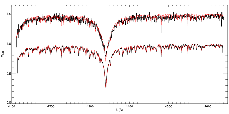
Figure 5: SME model fits (thin lines, red/grey) to the disentangled spectra (thick lines, black) of WASP 1628+10 A and WASP 1628+10 B (offset by +0.5 units).

3.3.2 Spectral energy distribution

We have also estimated the effective temperatures of the stars by comparing the observed flux distribution to synthetic flux distributions based on the BaSel 3.1 library of spectral energy distributions (Westera et al., 2002). Near-ultraviolet (NUV) and far-ultraviolet (FUV) photometry was obtained from the GALEX GR6 catalogue (Morrissey et al., 2007). Optical photometry was obtained from the NOMAD catalogue (Zacharias et al., 2004). Near-infrared photometry was obtained from the 2MASS and DENIS catalogues (Skrutskie et al., 2006; The DENIS Consortium, 2005). We used the calibration of Camarota & Holberg (2014) to correct the GALEX fluxes to account for the detector dead-time correction for bright stars. We assumed surface gravity values of $\log{\mathrm{g}}_{\mathrm{A}}=4.25$ for WASP 1628+10 A and $\log\mathrm{g}_{\mathrm{B}}=4.5$ for WASP 1628+10 B. The total line-of-sight reddening for WASP 1628+10 from the maps of Schlafly & Finkbeiner (2011) is E(B$-$V)=0.056 and our estimated standard error on this value is 0.034 magnitudes (Maxted et al., 2014). Additional constraints included in the fit are the observed values of the luminosity ratio, $\ell_{\rm r^{\prime}}$, and and surface brightness ratio, $J_{\rm r^{\prime}}$, from the fits to the r’-band lightcurves given in Table 3. Further details of the method are given in Maxted et al. (2014).

Based on the results of the spectral analysis above we restrict the comparision of the observed fluxes to models in which the metallicity of WASP 1628+10 A is [Fe/H]=$-0.5$ or [Fe/H]=$0$. The results are quite sensitive to the assumed reddening to the system and so we also imposed the value of T${}_{\rm eff,A}=7500\pm 200$ K from the analysis of the disentangled spectra as a constraint and only use the analysis of the spectral energy distribution to estimate the value of T_eff,B. With these constraints we find T${}_{\rm eff,B}=9800\pm 300$ K. The fit to the observed fluxes is shown in Fig. 6.

Figure 6: Model fit to the observed flux distribution of WASP 1628+10 used to estimate the effective temperatures of WASP 1628+10 B. The observed fluxes are shown as circles with error bars. The predicted contributions of each star to the observed fluxes are shown as dotted or dashed lines and their sum is shown as a solid line. The models have been smoothed slightly for clarity in these plots. Diamonds show the result of integrating the total model flux over the band-width indicated by horizontal error bars on the observed fluxes. The assumed band-width of the r’ filter is indicated with vertical dotted lines. The model for WASP 1628+10 A has $\mbox{T${}_{\mathrm{eff}}$}=7400$ K [Fe/H]=$-0.5$ and $\log\,{\mathrm{g}}$=4.25. The model for WASP 1628+10 B has $\mbox{T${}_{\mathrm{eff}}$}=9800$ K,[Fe/H]=$-0.5$ and $\log\,{\mathrm{g}}$=4.5. A reddening of E(B$-$V)=0.056 has been assumed.

3.4 Absolute parameters

The mass, radius, luminosity and other parameters of WASP 1628+10 A and WASP 1628+10 B based on the results above are given in Table 6. The adopted value of ${\rm T}_{\rm eff,B}$ is the average of the values derived from fitting its spectrum and from fitting the spectral energy distribution. The quoted error on this value reflects the difference between these two estimates.

Table 6: Physical parameters of WASP 1628+10 A and WASP 1628+10 B inferred from our observations. V_synch is the equatorial rotation velocity assuming synchronous rotation.

Parameter	WASP 1628+10 A	WASP 1628+10 B
Mass[${M}_{\sun}$]	$1.36\pm 0.05$	$0.135\pm 0.02$
Radius [${R}_{\sun}$]	$1.57\pm 0.02$	$0.348\pm 0.008$
Teff[K]	$7500\pm 200$	$9200\pm 600$
$\log L/\mbox{${L}_{\sun}$}$	$0.85\pm 0.05$	$-0.1\pm 0.1$
$\log\,{\mathrm{g}}$(cgs)	$4.18\pm 0.01$	$4.49\pm 0.05$
Vsynch [${\mathrm{km}\,\mathrm{s}}^{-1}$]	$110\pm 2$	$24\pm 1$
$[{\rm Fe/H}]$	$-0.3\pm 0.3$	$0.0\pm 0.4$

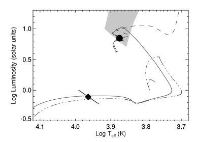
Figure 7: WASP 1628+10 A (circle) and WASP 1628+10 B (diamond) in the Hertzsprung-Russell diagram. The dashed line is a model for a star with a mass of 1.36${M}_{\sun}$ and metallicity Z=0.006. The solid line is a model for a star with an initial mass of 1.30${M}_{\sun}$ in a binary system with a 0.8${M}_{\sun}$ companion, orbital separation of 4.8${R}_{\sun}$  and metallicity Z=0.004. The dot-dash line is a model for a star with an initial mass of 1.0${M}_{\sun}$ in a binary system with a 0.9${M}_{\sun}$ companion, orbital separation of 4.8${R}_{\sun}$  and metallicity Z=0.008. The instability strip for $\delta$-Scuti-type pulsations with radial order $k=4$ is indicated by light-grey shading (Dupret et al., 2004).

4 Discussion

In Fig. 7 we show WASP 1628+10 A and WASP 1628+10 B in the Hertzsprung-Russell diagram (HRD) compared to various models produced with the garstec stellar evolution code (Weiss & Schlattl, 2008). We compared WASP 1628+10 A to a grid of models for single stars over a finely-sampled grid of stellar masses previously produced with garstec for the determination of stellar parameters from spectro-photometric and asteroseismic data (Serenelli et al., 2013). The properties of WASP 1628+10 A are well matched by stellar models of the appropriate mass and with a composition consistent with the value derived in Section 3.3.1. Models with solar composition are also a reasonable match to the observed position of this star on the HRD if the mass is assumed to be towards the lower limit allowed by our observations, or if we assume an enhanced helium abundance and solar metalicity for this star. It is likely that this star has accreted a substantial fraction of its current mass from its companion during the formation of the pre-He-WD. With better quality data it may be possible to detect surface composition anomalies or other signatures of the accretion history of this star.

For WASP 1628+10 B we created a grid of models using a modified version of garstec that accounts for Roche lobe overflow (RLOF) in binary evolution by forcing the radius of the star to match the radius of the Roche lobe during the semi-detached evolutionary phase. The grid of models comprises about 3000 evolutionary tracks. The mass of the donor ranges from 1.0 to 1.5 M_⊙ in steps of 0.1 M_⊙ for metallicity values $Z=0.004,0.008,0.012,0.016,0.020$. The mass of the original secondary star (now WASP 1628+10 A) ranges from 0.7 to 1.5 M_⊙ (also in steps of 0.1 M_⊙) and the orbital separation at the time mass transfer begins ranges from 4 to 5 R_⊙ in steps of 0.1 R_⊙. The orbital evolution is followed as described in Maxted et al. (2013), with mass loss and magnetic braking as the two mechanisms responsible for extracting angular momentum from the system. It is assumed that mass lost from the systems carries away all its angular momentum, and we assume a fraction $f=0.5$ of the mass lost by the donor is accreted onto the secondary.

A large number of these models match the observed properties of WASP 1628+10 B within the current large uncertainties on the mass and temperature of this star. Two such models are shown in Fig. 7, one of which has the correct mass and composition to be a good match in its early evolutionary phases to the current properties of WASP 1628+10 A. We did not find any models that can fit the properties of WASP 1628+10 B and that also match the orbital period of the binary – the models predict orbital periods less than about 0.4 days. This may be a result of the assumptions made in our model about the way that the star reacts to mass loss. If the star has a larger radius than assumed during the mass loss phase then the prediced orbital period predicted will also be increased. We have not explored this problem further, but this will certainly be a worthwhile exercise once we have stronger constraints on the mass, temperature and luminosity of this star.

The high-frequency signals we have detected in our Ultracam photometry are likely to be due to pulsations in WASP 1628+10 B similar to those seen in WASP 0247$-$25 B, i.e., a mixture of non-radial and radial overtone modes with p-mode characteristics in the envelope and g-mode characteristics in the interior of the star. These pulsations can enable detailed studies to be made of the interior of a star if the exact frequencies and oscillation modes can be identified, particularly if strong observational constraints on the mass, temperature and luminosity of the star are available.

Our models for the formation of WASP 1628+10 B do not include microscopic diffusion. In the models including diffusion that we computed for WASP 0247$-$25 B we found that the surface abundance of metals dropped to almost zero by the time the effective temperature of the star had risen to $\sim 7500$ K due to gravitational settling. The timescale for gravitational settling is expected to be similar for WASP 1628+10 B. The presence of a strong Mg II 4481Å line in the spectrum of WASP 1628+10 B shows that some process counteracts or prevents gravitational settling in its atmosphere. Radiative levitation may play a role in maintaining a metal-rich atmosphere, but it is also possible that the contraction of this star as it evolves to higher effective temperature produces an angular velocity gradient that drives rotation-induced mixing. It may be possible to study this issue in much greater detail if it can be confirmed that the high-frequency pulsations we have observed originate from pulsational modes in WASP 1628+10 B that show rotational splitting.

References

- Althaus et al. (2001) Althaus L. G., Serenelli A. M., Benvenuto O. G., 2001, MNRAS, 323, 471
- Barklem et al. (1998) Barklem P. S., Anstee S. D., O’Mara B. J., 1998, PASA, 15, 336
- Bíró & Nuspl (2011) Bíró I. B., Nuspl J., 2011, MNRAS, 416, 1601
- Bogdanovic et al. (2013) Bogdanovic T., Cheng R. M., Amaro-Seoane P., 2013, ApJ (submitted)
- Camarota & Holberg (2014) Camarota L., Holberg J. B., 2014, MNRAS
- Chen & Han (2003) Chen X., Han Z., 2003, MNRAS, 341, 662
- Claret (2004) Claret A., 2004, A&A, 428, 1001
- Dhillon et al. (2007) Dhillon V. S., Marsh T. R., Stevenson M. J., Atkinson D. C., Kerry P., Peacocke P. T., Vick A. J. A., Beard S. M., Ives D. J., Lunney D. W., McLay S. A., Tierney C. J., Kelly J., Littlefair S. P., Nicholson R., Pashley R., Harlaftis E. T., O’Brien K., 2007, MNRAS, 378, 825
- Driebe et al. (1999) Driebe T., Blöcker T., Schönberner D., Herwig F., 1999, A&A, 350, 89
- Dupret et al. (2004) Dupret M.-A., Grigahcène A., Garrido R., Gabriel M., Scuflaire R., 2004, A&A, 414, L17
- Etzel (1981) Etzel P. B., 1981, in E. B. Carling & Z. Kopal ed., Photometric and Spectroscopic Binary Systems A Simple Synthesis Method for Solving the Elements of Well-Detached Eclipsing Systems. p. 111
- Giannone & Giannuzzi (1970) Giannone P., Giannuzzi M. A., 1970, A&A, 6, 309
- Heiter et al. (2002) Heiter U., Kupka F., van’t Veer-Menneret C., Barban C., Weiss W. W., Goupil M.-J., Schmidt W., Katz D., Garrido R., 2002, A&A, 392, 619
- Horne (1986) Horne K., 1986, PASP, 98, 609
- Iben & Livio (1993) Iben Jr. I., Livio M., 1993, PASP, 105, 1373
- Kawka & Vennes (2009) Kawka A., Vennes S., 2009, A&A, 506, L25
- Kennelly et al. (1998) Kennelly E. J., Brown T. M., Kotak R., Sigut T. A. A., Horner S. D., Korzennik S. G., Nisenson P., Noyes R. W., Walker A., Yang S., 1998, ApJ, 495, 440
- Kilic et al. (2007) Kilic M., Allende Prieto C., Brown W. R., Koester D., 2007, ApJ, 660, 1451
- Kilic et al. (2012) Kilic M., Brown W. R., Allende Prieto C., Kenyon S. J., Heinke C. O., Agüeros M. A., Kleinman S. J., 2012, ApJ, 751, 141
- Knigge et al. (2008) Knigge C., Dieball A., Maíz Apellániz J., Long K. S., Zurek D. R., Shara M. M., 2008, ApJ, 683, 1006
- Landstreet et al. (2009) Landstreet J. D., Kupka F., Ford H. A., Officer T., Sigut T. A. A., Silaj J., Strasser S., Townshend A., 2009, A&A, 503, 973
- Lenz & Breger (2005) Lenz P., Breger M., 2005, Communications in Asteroseismology, 146, 53
- Lorimer (2008) Lorimer D. R., 2008, Living Reviews in Relativity, 11, 8
- Marsh et al. (1995) Marsh T. R., Dhillon V. S., Duck S. R., 1995, MNRAS, 275, 828
- Maxted et al. (2014) Maxted P. F. L., et al., 2014, MNRAS, 437, 1681
- Maxted et al. (2013) Maxted P. F. L., Serenelli A. M., Miglio A., Marsh T. R., Heber U., Dhillon V. S., Littlefair S., Copperwheat C., Smalley B., Breedt E., Schaffenroth V., 2013, Nature, 498, 463
- Morrissey et al. (2007) Morrissey P., et al., 2007, ApJS, 173, 682
- Nelson & Eggleton (2001) Nelson C. A., Eggleton P. P., 2001, ApJ, 552, 664
- Nelson et al. (2004) Nelson L. A., Dubeau E., MacCannell K. A., 2004, ApJ, 616, 1124
- Oke (1990) Oke J. B., 1990, AJ, 99, 1621
- Pollacco et al. (2006) Pollacco D. L., et al., 2006, PASP, 118, 1407
- Popper & Etzel (1981) Popper D. M., Etzel P. B., 1981, AJ, 86, 102
- Refsdal & Weigert (1969) Refsdal S., Weigert A., 1969, A&A, 1, 167
- Schlafly & Finkbeiner (2011) Schlafly E. F., Finkbeiner D. P., 2011, ApJ, 737, 103
- Serenelli et al. (2013) Serenelli A. M., Bergemann M., Ruchti G., Casagrande L., 2013, MNRAS, 429, 3645
- Simon & Sturm (1994) Simon K. P., Sturm E., 1994, A&A, 281, 286
- Skrutskie et al. (2006) Skrutskie M. F., et al., 2006, AJ, 131, 1163
- Southworth (2010) Southworth J., 2010, MNRAS, 408, 1689
- The DENIS Consortium (2005) The DENIS Consortium 2005, VizieR Online Data Catalog, 2263, 0
- Valenti & Piskunov (1996) Valenti J. A., Piskunov N., 1996, A&AS, 118, 595
- Webbink (1975) Webbink R. F., 1975, MNRAS, 171, 555
- Weiss & Schlattl (2008) Weiss A., Schlattl H., 2008, Ap&SS, 316, 99
- Westera et al. (2002) Westera P., Lejeune T., Buser R., Cuisinier F., Bruzual G., 2002, A&A, 381, 524
- Willems & Kolb (2004) Willems B., Kolb U., 2004, A&A, 419, 1057
- Zacharias et al. (2004) Zacharias N., Monet D. G., Levine S. E., Urban S. E., Gaume R., Wycoff G. L., 2004, in American Astronomical Society Meeting Abstracts Vol. 36 of Bulletin of the American Astronomical Society, The Naval Observatory Merged Astrometric Dataset (NOMAD). pp 1418–+