Diffractive wave guiding of hot electrons by the Au (111) herringbone reconstruction

Abstract

The surface potential of the herringbone reconstruction on Au(111) is known to guide surface-state electrons along the potential channels. Surprisingly, we find by scanning tunneling spectroscopy that hot electrons with kinetic energies twenty times larger than the potential amplitude (38 meV) are still guided. The efficiency even increases with kinetic energy, which is reproduced by a tight binding calculation taking the known reconstruction potential and strain into account. The guiding is explained by diffraction at the inhomogeneous electrostatic potential and strain distribution provided by the reconstruction.

I introduction

Electromagnetic waves can be steered phase-coherently along interfaces of different dielectric constant.Ghatak An analogous process of wave guiding is not well established for ballistic electrons, e.g. in nanostructures. Instead, hard-wall potentials, Beenakker ; vanWees ; Song ; McNeil or magnetic fields,Baranger ; Geim97 which confine the electron path classically, are invoked. However, exploiting the wave character of the electrons for steering might be less invasive for the phase information with obvious consequences for the transport of entangled quantum information.Beth ; Hansel Here, we probe the model system Au(111), for which the well-known herringbone reconstructionBarth90 provides a low-amplitude ($W_{\rm HB}=38$ meV) piecewise straight channeling potential with typical channel length of $l_{\rm HB}\approx 30$ nm.Crommie98 ; Kern02 The channeling potential is periodic transverse to the channel direction with period $\lambda_{\rm HB}=6.3$ nm. Previous scanning tunneling microscopy (STM) revealed standing electron waves preferentially along the channeling potential at a kinetic energy of $E_{\mathrm{kin}}:=E-E_{\Gamma}\approx 500$ meV ($E_{\Gamma}=-480$ meV, bottom of the surface band measured relative to the bulk Fermi level $E_{\rm F}$), which implies guiding of hot surface electrons.Fujita97 However, a satisfactory explanation has remained elusive: subsequent determination of the small amplitude of the reconstruction potential,Crommie98 ; Kern02 with $E_{\mathrm{kin}}/W_{\rm HB}\gtrsim 10$ rule out the originally proposed modelFujita97 ; Fujita973 of guiding by channeling in the potential well. Indeed, the channeling interpretation has been challenged by showing that the Talbot effect arising at an undulated step edge reveals a similar standing wave pattern.Wenderoth On the other hand, anisotropic standing wave patterns have not been found for surface states on unreconstructed close-packed surfaces as Cu(111), Ag(111), Pt(111) or Ni(111).Petersen98 ; Jeandupeux99 ; Wiebe05 ; Braun08

Here, we present a novel explanation of the guiding at high energies: the regular dislocation lines act as a diffractive grating, leading to a zeroth-order diffraction peak in the direction along the reconstruction lines, and thus to diffractive focusing in momentum space. Using STM and scanning tunneling spectroscopy (STS), we probe the Au (111) surface state and identify two energy regimes: at low energies, $E_{\mathrm{kin}}\lesssim W_{\rm HB}$, electrons channel within the hexagonal close-packed (hcp) regions of the reconstruction as originally proposed. At higher energies up to $E_{\mathrm{kin}}/W_{\rm HB}>20$, the electrons still propagate anisotropically, i.e. preferentially along the reconstruction lines, but in all regions of the sample and not only in the hcp regions. Diffraction explains both the large energy $E_{\mathrm{kin}}/W_{\rm HB}\gg 1$ of steered electrons and the absence of a preferential stacking area for wave guiding.

To uncover the ingredients of the guiding effect, we perform tight binding (TB) simulations of the local density of states (LDOS). Quantitative agreement between simulations and experimental data requires to include the measured electrostatic potential of the surface reconstruction,Kern02 the change in effective mass due to the known compressive strain at the dislocation lines,DFT_GOLD1 and disorder scattering at point defects. Without strain, the guiding effect would still be present but weaker than in the experiment. Finally, we present a semiclassical model for the interference of different electron paths subject to reflection at the reconstruction lines and impurities. This model qualitatively reproduces the effect, further corroborating that diffraction is, indeed, the origin of the guiding. Similar partial dislocation lines exist in other structures, e.g., multilayer graphene.Ping ; Hattendorf ; Alden Our present findings for Au(111) may therefore open the door to non-dispersive wave guiding for electrons by diffraction in such structures.

II Experiment

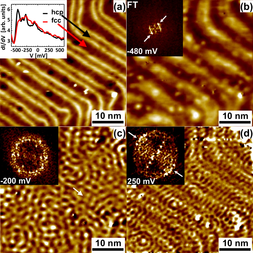
Figure 1: (color online) (a) STM image of Au(111), $I=1\rm\,nA$, $V=-480\rm\,mV$; herringbone reconstruction and a few impurities (bright and dark spots) are visible. Inset: Spatially averaged $dI/dV$ spectra taken on hcp and fcc areas as indicated by arrows, $I_{\rm stab}=1\rm\,nA$, $V_{\rm stab}=-540$ mV, $V_{\rm mod}=10\rm\,mV$. (b)-(d) $dI/dV$ maps of the same surface area as in (a) recorded in constant-current mode at voltages as marked in the insets, $I=1\rm\,nA$, $V_{\rm mod}=10\rm\,mV$. Arrow in (c) indicates a guided standing wave. Insets: Fourier transformations (FT) of the $dI/dV$ images; arrows in (b) mark spots corresponding to the herringbone periodicity; arrows in (d) mark the enhanced intensity within the circle in the direction parallel to the reconstruction lines.

The STM/STS experiments are performed in ultrahigh vacuum at 5 K.Mashoff09 The Au(111) surface is prepared by cycles of Ar ion sputtering ($p_{\mathrm{Ar}}=1-3\cdot 10^{-5}\rm\,mbar$, $E_{\mathrm{ion}}=700\rm\,eV$) and annealing ($T=450\,^{\circ}$C, $\sim 10$ min).Barth90 ; Crommie98 ; Wenderoth After the preparation, the sample is transferred into the precooled STM. STM images and $dI/dV$ maps, the latter recorded by lock-in-technique with modulation voltage $V_{\rm mod}$, are taken in constant-current mode at current $I$ and sample voltage $V$. The $dI/dV$ curves are recorded with open feedback after stabilizing the tip at current $I_{\rm stab}$ and voltage $V_{\rm stab}$.

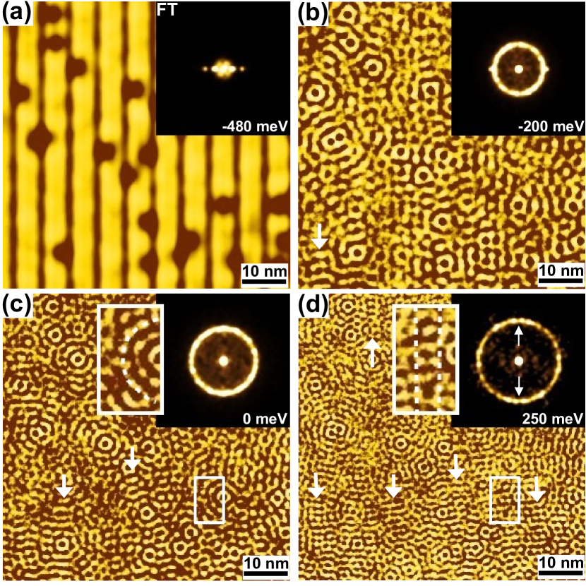
Figure 2: (color online) Calculated LDOS maps at $E-E_{\rm F}$ as marked in the subfigures; reconstruction lines run vertically; insets in upper right corner are FTs of the real space images; arrows in LDOS images mark standing waves running along the reconstruction lines; pairs of white rectangles in (c) and (d) show a region close to a point scatterer and the corresponding zoom-in: wave guiding is visible at 250 mV, but not at 0 mV; arrows in FT point to the increased intensity along the reconstruction; the TB calculation includes the electrostatic potential and the strain of the reconstruction lines as well as impurities modeled as Gaussian potentials with amplitude 2.5 eV and width 0.3 nm.

STM images of Au(111) [Fig. 1(a)] exhibit the well-known $23\times\sqrt{3}$ herringbone reconstruction consisting of alternating regions of hexagonal close-packed (hcp) and face-centered cubic (fcc) stacking separated by bright partial dislocation lines.Woell89 ; Barth90 ; Wenderoth Additionally, a few impurities are visible as bright spots. The $dI/dV$ curves [Fig. 1 (a), inset] reproduce the well-known differences in the electronic structure between hcp and fcc areas.Crommie98 FTs of $dI/dV$ maps recorded at different $V$ in steps of $50\,$mV [see Appendix A for a gallery] reveal the well-known parabolic dispersion of the Au(111) surface stateKevan ; LaShell with the origin at $E_{\Gamma}=-480$ meV and an effective mass $m^{\star}\simeq 0.25m_{\mathrm{e}}$ [as shown in Ref. GeringerPhD, ], in good agreement with previous photoemissionKevan as well as scanning tunneling spectroscopySchouteden ; Kern02 results. We also reproduce the multiple phase shifts of the intensity distribution perpendicular to the reconstruction lines which indicate miniband formation.Didiot07 ; Didiot072 ; Didiot10 ; GeringerPhD Here, we focus on the anisotropy of standing waves visible in the $dI/dV$ maps [see Fig. 1]. The higher $dI/dV$ intensity at $-480\,$mV in hcp areas [Fig. 1(b)] is caused by localization of surface electrons in regions of lower electrostatic potential.Fujita97 ; Crommie98 ; Kern02 The 2D Fourier transformation (FT) of the $dI/dV$ map shows only spots related to the periodicity of the surface reconstruction [Fig. 1(b), inset]. The $dI/dV$ maps between -400 mV and -150 mV corresponding to $E_{\mathrm{kin}}>W_{\rm HB}$ reveal ringlike standing electron waves around point-like scatterers [see Fig. 1(c)] as expected for isotropically delocalized electrons.Heller94 ; Crommie93 ; Wittneven In between, interference patterns due to the random superposition of plane waves appear as typical for 2D scattering.Morg02 The FT, accordingly, shows a largely isotropic ring-like distribution of contributing electronic wave vectors $\mathbf{k}$ [Fig. 1(c), inset].

At higher energies ($V\gtrsim-150\,$mV, $E_{\mathrm{kin}}\gtrsim 330\,$meV) [Fig. 1(d)], the electron standing waves become increasingly oriented along the direction of the herringbone channels and much less in the transverse direction. Hence, the FT exhibits a ring with anisotropic intensity being largest in the direction parallel to the reconstruction lines as marked by arrows. The standing waves along the reconstruction exist within the fcc and hcp regions which excludes potential channeling as the origin of the guiding effect [Appendix B].

III Simulation

To uncover the physical origin of guiding, we simulate the electronic structure of the Au (111) surface band using a tight-binding description in the continuum limit.MUMPS We include the herringbone reconstruction as a one-dimensional periodic on-site potential

$$W = \frac{W_{\rm HB}}{2}\left[1+\cos^{2}\left(\frac{1}{2}k_{\rm HB}x\right)\right]\cos^{2}(k_{\rm HB}x)$$ (1)

with $W_{\rm HB}=$38 $\mathrm{meV}$ the height of the reconstruction potential and $k_{\rm HB}=2\pi/6.3$ nm^-1 its fundamental wave vector as measured by Ref. Kern02, . In order to include the known compressive lateral strain variation within the reconstruction,DFT_GOLD1 we perform ab-initio density functional theory calculations of unreconstructed Au(111) with varying lattice spacings. We use the VASP software package,KresseFuerthau including the associated PAW potential for gold, and the PBE XC functional.PBE We perform a geometry relaxation of a 1x1 fcc (111) surface slab containing 11 layers [i.e. 11 atoms in the unit cell] in a unit cell containing 20 Å vacuum between the periodic images of the layer. For $k$-point sampling in the slab, we use a Monkhorst-Pack grid of $18\times 18\times 1$. We relax the three top and bottom layers. Finally, we calculate for the optimized geometry the surface band structure, and identify the gold (111) surface state. We deduce the $m^{\star}$-dependence on strain by fitting the resulting parabolic dispersion $E_{\mathrm{kin}}=\hbar^{2}{\bf k}^{2}/(2m^{\star})$ ($\hbar$: Planck’s constant). From the literature DFT_GOLD1 ; DFT_GOLD2 the lattice constant within the reconstructed top layer is known to vary around the equilibrium lattice constant with the same period as the reconstruction: the functional form is similar to the variation in the on-site potential, Eq. (1), with a strain amplitude of about 2%. Accordingly, we investigate the variations in the dispersion relation of the surface state as a function of the stretching of the fcc lattice in the (100) direction up to 2%. We find a variation of the lower band edge of the order of 40 meV, in agreement with the amplitude of the on-site potential of Eq. (1). We also find a variation in the effective mass $m^{\star}$ [in the (100) direction] of the surface state of $4\%$ for the largest strain of $2\%$. Such a change in effective mass corresponds to a variation in the hopping parameter and the on-site element of our tight-binding simulation to obtain the correct continuum limit.

We account for disorder by including randomly distributed point-like scattering potentials with a concentration $n\approx 0.01\,/{\rm nm}^{2}$ as taken from the STM measurements. We use narrow Gaussian peaks of height 2.5 eV and width $W\approx 3$ Å. The results were found to only weakly depend on the exact shape of the scattering potentials, as long as their characteristic length scale is short compared to the electron wavelength. Scattering by phonons and electron-electron interaction has been found to exhibit a mean free path $l_{\rm MFP}$ exceeding 30 nm in the investigated energy range and is thus of minor importance.Reinert01 ; Echenique04 ; Campillo00 The finite length of the herringbone channels $l_{\rm HB}$ does not explicitly enter the calculation except for the requirement that the length $L$ of the patch calculated satisfies $L\gtrsim l_{\rm HB}\gg\lambda_{\rm HB}$. We use an approximately quadratic patch of 150$\times$150 nm² with randomly shaped, soft-walled boundaries (roughness amplitude $12\,$nm) to avoid unphysically preferred directions due to boundary effects. The LDOS of the patch is deduced by summing the calculated electronic eigenstates over an energy window of 25 meV (about 250 eigenstates at $E_{\mathrm{kin}}=-0.2$ eV), in line with the experimental energy resolution. Superposing the squared eigenstates yields an LDOS at $E$. Fig. 2 shows LDOS maps and corresponding FTs of the central area ($65\times 65$ nm²) of a particular patch (for a gallery see Appendix A. Fig. 7). The calculated maps resemble the experimental LDOS maps in Fig. 1(b)-(d): channeling within the hcp regions at low energy [Fig. 2(a)], mostly isotropic scattering with some regions of wave guiding (arrows) at intermediate energies [Fig. 2(b)(c)] and increasingly preferential standing waves along the reconstruction lines at higher energy [Fig. 2(d)]. The FTs exhibit rings with angular anisotropy being most obvious at the highest energy (arrows). The maximum FT intensity is in the direction along the reconstruction lines. A zoom into an area close to a point scatterer [see white rectangles in Fig. 2(c) and (d)] provides a real-space visualization for the increase of guiding with energy: the standing waves encircle the nearest defect in (c), while the ladder-like interference pattern in (d) is formed by a standing wave running along the reconstruction lines.

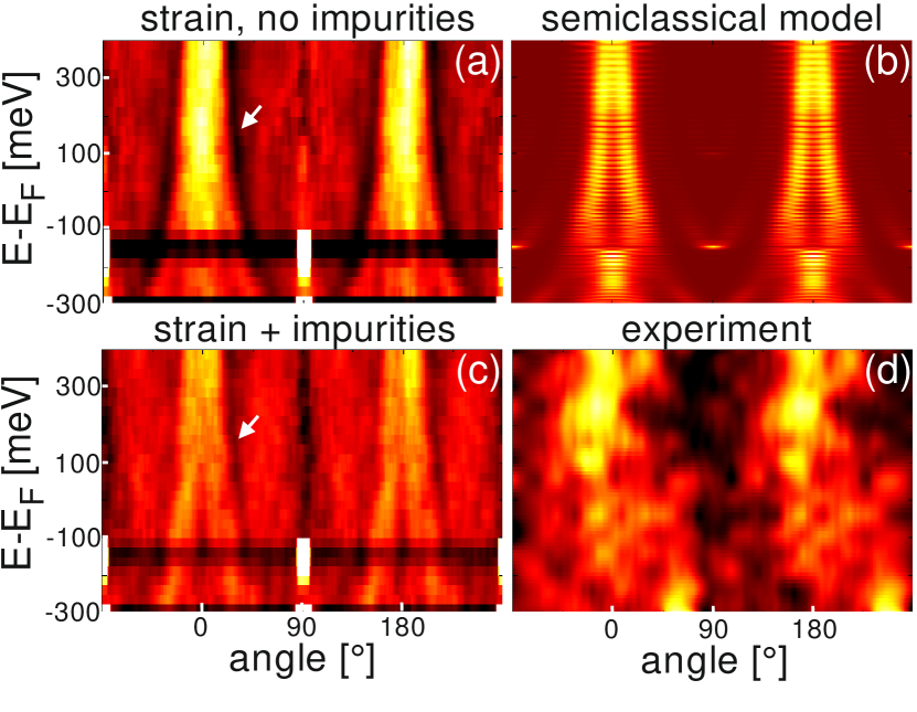
Figure 3: (color online) Colorplot of the angular distribution of the FT averaged around the dominant $|{\mathbf{k}}|$ (ring structure in FTs of Fig. 1 and 2, respectively, Fig. 6 and 7: (a) FT from ideal theoretical LDOS including reconstruction potential and strain but no disorder; (b) angular and energy dependence of backscattering probability according to a semiclassical Gutzwiller path calculation of the LDOS including reconstruction potential, strain and impurities (random phase shift of wave at each impurity $|\beta_{R}|<0.05\pi$); (c) same as (a) but with impurities as in Fig. 2 and Fig. 7; (d) FT from experimental LDOS for one domain of the herringbone reconstruction after angular smoothing (2nd order polynomial fit) and setting $eV=E-E_{\rm F}$. The color scale in all images covers the range [0.52, 1.00]; arrows at the dark lines in (a),(c) mark the dominant diffractive minimum [Eq. (2)]; all theoretical FTs are averaged over 50 realizations of disorder and different edge configurations for each energy, after subtracting the LDOS of a calculation with the same boundary, but without reconstruction or impurities, in order to remove the remaining influence of the boundary.

IV Comparison between experiment and simulation

In order to quantify the correspondence between STS data and TB data, we consider the angular-resolved FT intensity around the dominant $|\mathbf{k}|$ (ring in the insets of Fig. 1 and 2) as a function of energy: FT$(\alpha,E)$ [Fig. 3]. To remove any residual numerical artifacts from the grid or boundary directions within the calculation, we subtract for each patch the results from an identical calculation without any reconstruction potential or point scatterers. The subsequent average over 50 realizations further minimizes remaining interference effects between waves scattered from the boundary and from the reconstruction potential and impurities within the FT$(\alpha,E)$. TB calculations without [Fig 3(a)] and with impurities [Fig 3(c)] show a clear focusing effect, visible as a bright stripe around $0^{\circ}$ and $180^{\circ}$. The bright stripe gets sharper and more intense with increasing energy. Such an increase is expected for diffraction, since smaller wavelength (higher energy) decreases the angle of constructive interference for a given spacing of the grating. Consequently, a focusing around the forward direction in $k$-space appears. The maxima are, indeed, delimited by a stripe (arrows) indicating the lowest order diffractive minimum of the dominant Fourier component $2k_{\rm HB}$ of the reconstruction potential at

$$\sin\alpha=\frac{\hbar k_{\rm HB}}{2\sqrt{2E_{\mathrm{kin}}m^{\star}}}.$$ (2)

Without impurities the interference structure is more pronounced, as expected.

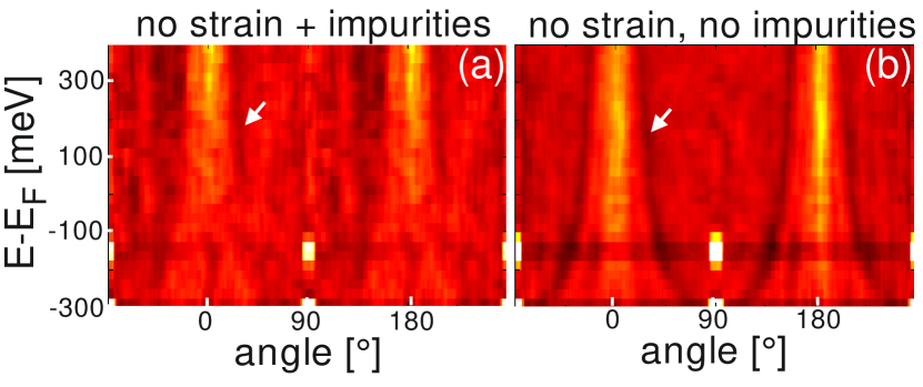
Figure 4: (color online) Angular dependence of the FT of theoretical LDOS maps, but in contrast to Fig. 3 without considering any strain effects (same color scale and contrast as in Fig. 3). (a) with and (b) without disorder scattering.

To elucidate the conditions required for the observation of electron wave guiding along the direction of the herringbone reconstruction pattern, we also perform a semiclassical simulation. We consider the interference pattern created by superposition of closed semiclassical orbits. We use the complex reflection and transmission amplitudes at a single period of the reconstruction potential to evaluate the weight and phase of semiclassical closed orbits based on a Gutzwiller trace formula.Brack The semiclassical action along each path $C$ is given by

$$S=\int_{C}kdq+\mu+\beta_{R}.$$ (3)

The phase $\mu\left(t(k),r(k)\right)$ accounts for the phase shifts accumulated by reflections at the reconstruction potential (similar to a Maslov index), and the (randomly determined) small angle $\beta_{R}\in[-\beta_{\max}(k),+\beta_{\max}(k)]$ accounts for random phases accumulated by impurity scattering. The weight of each path is determined by the accumulated reflection/transmission probabilities along the path. We include all combinations of multiple reflections at the periodic potential, for up to 16 internal reflections, until numerical convergence is reached. We use Gutzwiller’s trace formula to derive, from the superposed periodic orbits, the local density of states.Brack Upon summation of the different complex amplitudes associated with paths for a given starting angle $\alpha_{0}$ we obtain the angular distribution as a function of energy. We obtain the increased guiding of electrons at higher energies along the direction of the reconstruction lines [Fig. 3(b)]. Moreover, our model qualitatively reproduces (i) the dependence of the onset of wave guiding on the amount of dephasing by impurity scattering $\beta_{\max}$ and (ii) the dependence of the onset of wave guiding on the maximal allowed path length (limited in experiment by both the inelastic mean free path, and the length of the herringbone channel). Indeed, for high disorder concentration, the only remaining discernible feature is the zeroth-order diffraction peak. Due to the drastic approximations made in terms of modeling of impurity scattering as random phases and multiple scattering events at the herringbone potential, we do not expect exact quantitative agreement. Nevertheless, our semiclassical model supports the notion that the observed channeling is, indeed, a direct consequence of diffractive scattering of waves on the scattering grid created by the herringbone potential. We conclude that interference, i.e. diffraction, accounts for the effect.

The experimental FT$(\alpha,E)$ [Fig. 3(d)] shows striking similarities to TB calculations and the semiclassical model, i.e. a bright stripes around $0^{\circ}$ and $180^{\circ}$, which get stronger and sharper with increasing $E_{\mathrm{kin}}$. The reduced sharpness in the experiment is most likely due to angular smoothing required for noise suppression. Since the appearance of a pronounced diffractive minimum required averaging over 50 disorder realizations in the simulation for each energy, we do not expect to see it for a single series of experimental $dI/dV$ images. Note that the contrast of the experimental pattern is quantitatively similar to the calculated ones [Fig. 3]. Finally, calculations without considering the change in effective mass due to strain [see Fig. 4] show qualitatively similar features as with strain, yet feature a weaker contrast than the experiments and the calculations including strain. We thus conclude that strain is decisive to reproduce the strength of the guiding effect.

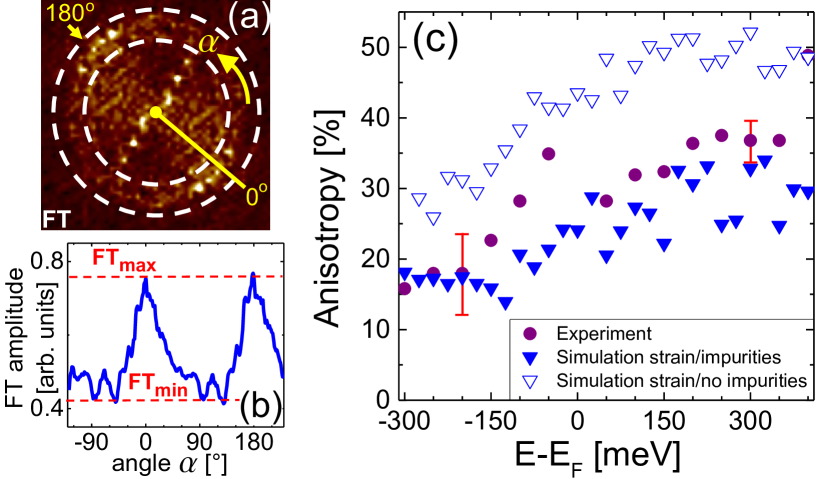
Figure 5: (color online) (a) FT of $dI/dV$ map at $V=250\rm\,V$ recorded within a single domain of the reconstruction lines; dashed rings border the area used for the angular plot in (b); angles of maximum intensity $\alpha=0\,^{\circ}$ and $\alpha=180\,^{\circ}$ are marked. (b) Angular distribution of FT amplitude radially averaged over the ring marked in (a); minimum FT_min and maximum FT_max are marked. (c) Anisotropy $A$ according to Eq. (4) from experimental data [circles] and from TB simulations ($\triangledown$: without, $\blacktriangledown$: with scatterers). Experimental error bars decrease with energy as indicated.

Figure 5 shows a direct quantitative comparison between experiment and TB simulation. We cut out the ring area of the FT belonging to standing waves [Fig. 5(a)], which results in the angular distribution FT$(\alpha)$ [Fig. 5(b)]. FT$(\alpha)$ displays pronounced maxima at the angles along the reconstruction lines. We define the anisotropy $A$ by

$$A:=\frac{\mathrm{FT}_{\max}-\mathrm{FT}_{\min}}{\mathrm{FT}_{\max}+\mathrm{FT}_{\min}}.$$ (4)

with $\mathrm{FT}_{\max}$ and $\mathrm{FT}_{\min}$ being the maximum and the minimum of $\mathrm{FT}(\alpha)$, respectively. Figure 5(c) reveals that the experimental data for $A$ increase with energy from $A<0.2$ at $E-E_{\rm F}\simeq-300$ mV to $A>0.35$ for $E-E_{\rm F}\simeq 350$ mV. The TB simulation without impurities reproduces the increase, but with absolute values of $A$ being larger than in the experiment. Including impurities reduces $A$ to reach a reasonable agreement with the experimental data. Neglecting the strain yields a strongly reduced anisotropy that only weakly increases with energy. Even without impurities we obtain $A=0.15$ at $E-E_{\rm F}\simeq-300$ mV and $A=0.2$ at $E-E_{\rm F}\simeq 400~{}$mV, i.e. values much lower than in experiment and barely increasing with energy. This emphasizes that strain contributes significantly to the guiding as can be rationalized by the influence of effective mass ($m^{\star}$) and on-site potential ($W$) on the parabolic energy dispersion. In other words, strain changes the curvature of a parabolic band, while the electrostatic potential only changes the origin of the parabola on the energy axis. Consequently, the distance of k-points at high energy is much larger in case of strain than in case of electrostatic potential. This implies a higher reflection coefficient in case of strain and, thus, a stronger guiding by the reconstruction, explaining the increase of intesity in FT$(\alpha,E)$ in forward direction with increasing energy (Fig. 3).

V Conclusion

In conclusion, we have presented a joint experimental and theoretical analysis of guiding of surface electrons on Au (111) by the herringbone reconstruction. We identify two energy regimes. At low energies, electrons assemble in the hcp channels of the reconstruction potential implying channeling. At higher energies above the confinement potential, the angular focusing into the direction of the channels is induced by diffraction. This focusing even increases with energy due to a locally varying effective mass induced by the strain distribution in the reconstruction. Remarkably, the guiding parallel to the herringbone channels persists up to energies that exceed the height of the reconstruction potential by a factor of 20.

Appendix A Comparison of measured and calculated LDOS images on Au(111)

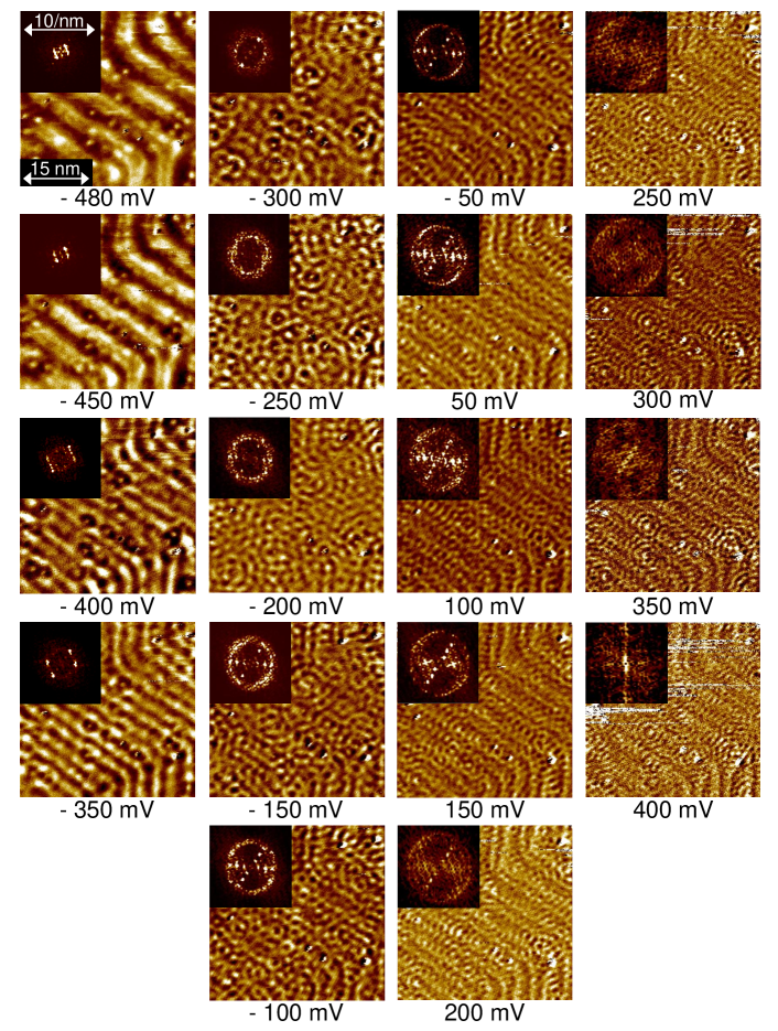
Figure 6: $dI/dV$ maps of the same surface area at voltages $V$ as marked below the images, $I=1\rm\,nA$, $V_{\rm mod}=10\rm\,mV$; Insets: Fourier transformations of the $dI/dV$ images; size of $dI/dV$ map and Fourier transformation are the same for all $V$; contrast is adapted to improve visibility.

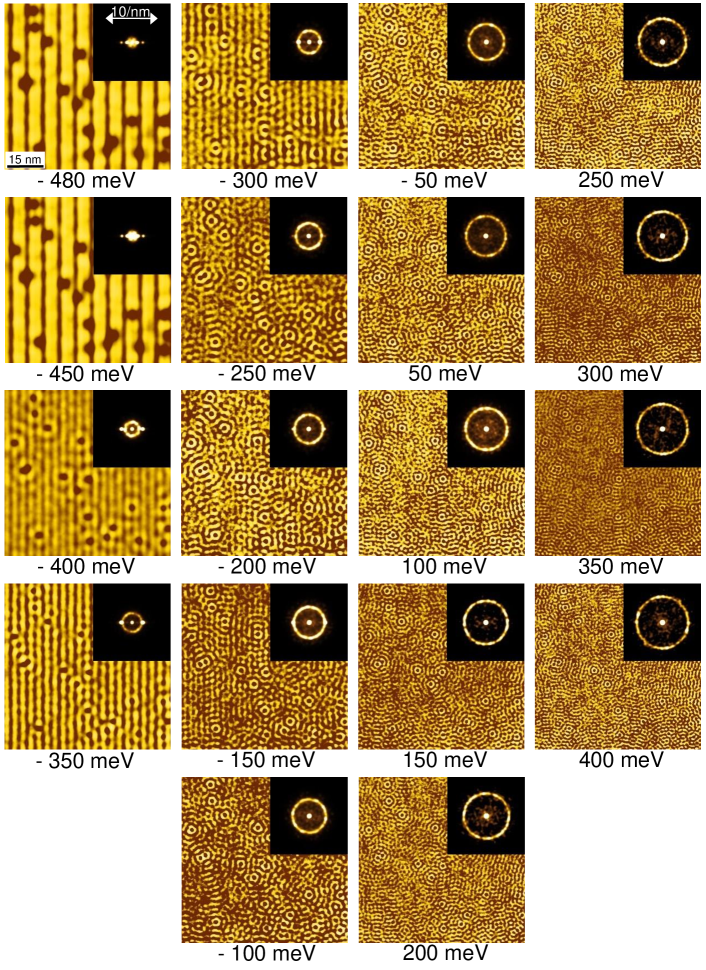
Figure 7: Theoretical LDOS maps at voltages $V$ as marked below the images for a particular configuration of impurities, compare with the experimental LDOS in Fig. 6. The reconstruction lines run from top to bottom. Insets: Fourier transformations of the $dI/dV$ images; size of $dI/dV$ map and Fourier transformation are the same for all $V$; contrast is adapted to improve visibility.

Figs. 6 shows experimental LDOS images of the same area of a Au(111) surface recorded at various energies (see insets). Fig. 7 shows the calculated LDOS patterns for comparison. The insets show the corresponding Fourier transformations (FTs). The images feature slightly varying contrast in order to improve visibility. Features in the experimental and theoretical data are largely identical, albeit the strength of the features coming directly from the reconstruction lines appear more intense in the experiment. At low voltage the confined states with nodes and antinodes perpendicular to the reconstruction lines dominate the LDOS map. Consequently, two pairs (one pair) of spots are visible in the experimental (calculated) FT. In experiment, the two pairs correspond to the two different domains visible in the main image. Between $-450$ and $-400$ mV, a doubling of antinodes is visible in the main image leading to a doubling of the distance between the pairs of spots in the experimental FT. The theoretical LDOS also features faint spots at larger distance and energies -480 and -450 meV. Notice that confinement of the electrons within the reconstruction potential of height 38 meV Crommie98 ; Kern02 is only present within the images recorded at $-480$ mV and $-450$ mV. At $-400$ mV and $-350$ mV, i.e. at energies above the confinement potential, first circular structures are visible around defects, which are attributed to standing electron waves. They lead to a faint circle within the FT exhibiting an increasing radius with increasing energy. Between $-300$ mV and $-200$ mV, this circle becomes more intense with respect to the spots from the reconstruction showing that the influence of the confinement potential gets weaker. The intensity within the circle is rather homogeneous indicating largely isotropic scattering of electron waves. This is also visible within the LDOS images, where no direction appears to be preferred by the electron waves. Above $-150$ mV, the two lines of spots within the circle, representing nodes and antinodes perpendicular to the reconstruction lines, get more intense again. In addition, the circular intensity within the FT becomes asymmetric with larger intensity in the upper left and the lower right region in experiment, and in the upper and lower region within the simulations. This brighter region is caused by the steering of the electron waves along the reconstruction lines, which is visible in the real space LDOS images too. The brighter area within the ring is composed of intensity perpendicular to the lines of spots originating from the reconstruction. To demonstrate this, the experimental FTs above $200$ mV are not taken from the whole image, but only from the area where reconstruction lines run diagonally through the image. Then, only one line of spots and the corresponding perpendicular bright areas within the ring appear. Thus, the transition from confined states at low energy to largely isotropic scattering at medium energies, and to a continuously increasing wave guiding at higher energies is clearly discernible in theory and experiment.

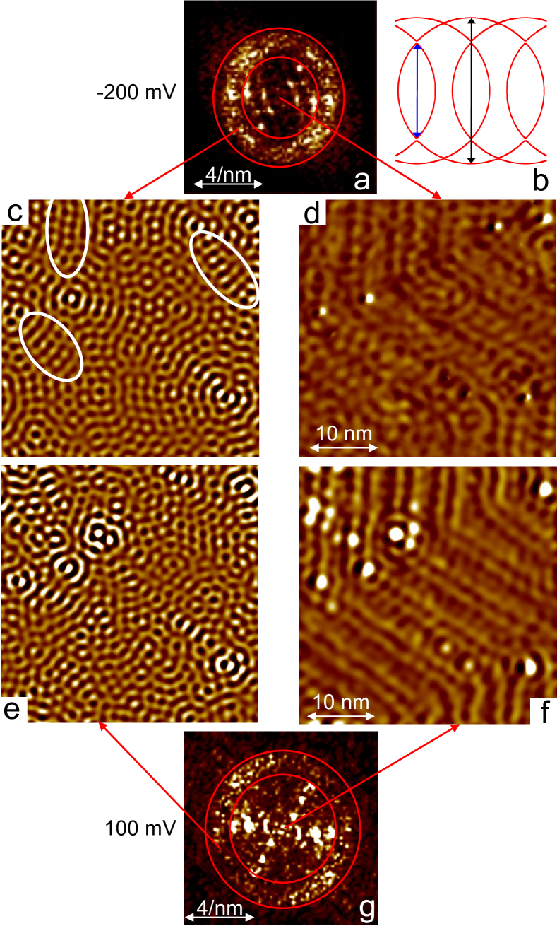
Figure 8: (a) Power spectrum of Fourier transformation of $dI/dV$ map recorded at $V=-200$ mV; regions for back-transformation in (c) and (d) are marked by red circles; (b) five backfolded constant-energy circles in $\mathbf{k}$ space for Au(111) with gaps originating from miniband formation and marked preferential scattering vectors parallel to the reconstruction lines (arrows); (c) Image resulting from inverse Fourier transformation of (a) after applying an ideal band-pass filter selecting the ring structure, which is bordered by the two red circles in (a); white circles mark areas of wave guiding; (d) Image resulting from inverse Fourier transformation of (a) after applying an ideal low-pass filter selecting the area bordered by the inner red circle; (e), (f) same as (c),(d) but for a $dI/dV$ image recorded at $V=100$ mV and backtransformed from (g); (g) Power spectrum of Fourier transformation of $dI/dV$ map recorded at $V=100$ mV; regions for back-transformation in (e) and (f) are marked by red circles.

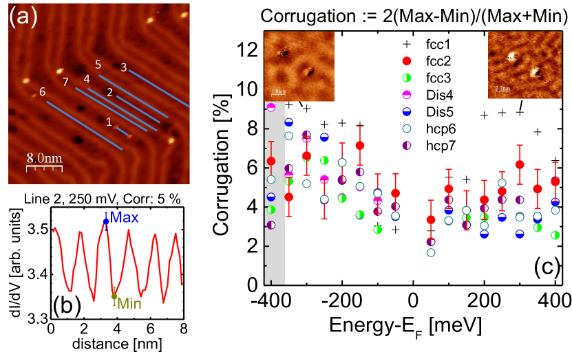
Figure 9: (a) STM image of Au(111), $I=1$ nA, $V=-0.48$ V with marked lines where the corrugation $C$ is measured. (b) $dI/dV$ intensity along line 2 in (a) recorded at $V=0.25$ V; minima (Min) and maxima (Max) as used for the evaluation of $C$ are marked. (c) Corrugation $C$ as determined by Eq. (5) as a function of electron energy with respect to $E_{\rm F}$ for the lines marked in (a); labels include the type of region (Dis = dislocation line) as well as the number marking the lines in (a); Insets show $dI/dV$ images corresponding to the marked points of relatively large corrugation; grey area marks the channeling energies; $I=1$ nA, $V_{\rm mod}=10$ mV for all data points and the insets.

A more detailed analysis of the contributions to the FT [Fig. 8] proves that the ring within the power spectrum of the FT is, indeed, caused by standing electron waves while the intensity spots at lower $\mathbf{k}$ are mostly due to the Au(111) reconstruction. To disentangle contributions of the guided electrons and the herringbone reconstruction, we partition the FT into the ring area around the Fermi circle, and its interior [see two red circles in in Fig. 8(a)]. We consider energies $V=-200$ mV [Fig. 8 (a)] and $V=100$ mV [Fig. 8(g)]. Both the ring and the circle are back-transformed separately into real-space images as indicated by arrows. The backtransformed images of the ring area are shown in Fig. 8(c) and (e) and the backtransformed images of the inner circle area are shown in Fig. 8(d) and (f). The $dI/dV$ images corresponding to the ring nicely show electron wave patterns which are regularly distributed over the surface. This regular distribution is typical for 2D states because of the larger probability for closed trajectories of the electrons on a path including several defects.Morg02 ; Morg
It is obvious that most of the electron wave patterns are isotropic in Fig. 8(b), but that wave guiding along the reconstruction lines already exists in certain areas of the sample as marked by white rings. This explains that the anisotropy shown in Fig. 3(c) does not drop to zero at lower energy. In Fig. 8(e) the wave guiding is evidently stronger. Notice that wave guided patterns of electron waves are also observed in Fig. 8(f) and (d). We believe, that this is due to the fact that band gaps open at the crossing points of different constant-energy circles (the original one and backfolded ones) as shown in Fig. 8(b), which implies additional scattering vectors along the reconstruction lines but with shorter wave vectors (blue arrow) than for scattering across the original circle (black arrow).

Appendix B Corrugation

We determine the corrugation of the standing electron waves along the reconstruction line for different perpendicular coordinates labeled by 1 to 7 in Fig. 9(a). Lines 1 to 3 are located in fcc regions, lines 4 and 5 on top of dislocation lines, and 6 and 7 in hcp regions. For each section line in $dI/dV$ images as shown, e.g. in Fig. 9(b), the maxima (Max) and minima (Min) determine the relative corrugation $C$ according to

$$C(E)=2\frac{(dI/dV)_{\max}-(dI/dV)_{\min}}{(dI/dV)_{\max}+(dI/dV)_{\min}}.$$ (5)

$C(E)$ is found to be largely independent of the stacking and, thus, of the local reconstruction potential [Fig. 9(c)], i.e. the observed steering is spatially homogeneous. This further corroborates that the steering effect is not a real-space channeling in regions of minimal potential. $C(E)$ depends also only weakly on energy, except where Fabry-Perot resonances between adjacent scatterers appear [see e.g. Line 1 in Fig. 9 connecting two adjacent defects]. Two resonances with larger $C(E)$ appear if one or two antinodes between the two defects are observed [see insets].