Parameters of cosmological models and recent astronomical observations
Abstract
For different gravitational models we consider limitations on their parameters coming from recent observational data for type Ia supernovae, baryon acoustic oscillations, and from 34 data points for the Hubble parameter depending on redshift. We calculate parameters of 3 models describing accelerated expansion of the universe: the CDM model, the model with generalized Chaplygin gas (GCG) and the multidimensional model of I. Pahwa, D. Choudhury and T.R. Seshadri. In particular, for the CDM model estimates of parameters are: km c-1Mpc-1, , , . The GCG model under restriction is reduced to the CDM model. Predictions of the multidimensional model essentially depend on 3 data points for with .
I Introduction
The most important challenge for cosmologists is to explain the accelerated expansion of our universe that was directly measured for the first time from Type Ia supernovae observations Riess98 ; Perl99 . These supernovae were used as standard candles, because one can measure their redshifts and luminosity distances . The observed dependence based on further measurements SNTable ; WeinbergAcc12 argues for the accelerated growth of the cosmological scale factor at late stage of its evolution.
This result was confirmed via observations of cosmic microwave background anisotropy WMAP , baryon acoustic oscillations (BAO) or large-scale galaxy clustering WeinbergAcc12 ; Eisen05 ; SDSS and other observations WeinbergAcc12 ; WMAP ; Plank13 . In particular, our attention should be paid to measurements of the Hubble parameter for different redshifts Simon05 ; Stern10 ; Moresco12 ; Blake12 ; Zhang12 ; Busca12 ; Chuang12 ; Gazta09 ; Anderson13 ; Oka13 ; Delubac14 ; Font-Ribera13 . The results of these measurements and estimations are represented below in Table 6 of Appendix.
The values were calculated with two methods: evaluation of the age difference for galaxies with close redshifts in Refs. Simon05 ; Stern10 ; Moresco12 ; Blake12 ; Zhang12 ; Busca12 ; Chuang12 and the method with BAO analysis Gazta09 ; Anderson13 ; Oka13 ; Delubac14 ; Font-Ribera13 .
In the first method the equality
| (1) |
and its consequence
are used. Here is the current value of the scale factor .
Baryon acoustic oscillations (BAO) are disturbances in the cosmic microwave angular power spectrum and in the correlation function of the galaxy distribution, connected with acoustic waves propagation before the recombination epoch WeinbergAcc12 ; Eisen05 . These waves involved baryons coupled with photons up to the end of the drag era corresponding to Plank13 , when baryons became decoupled and resulted in a peak in the galaxy-galaxy correlation function at the comoving sound horizon scale Eisen05 ; Plank13 .
In Table 5 of Appendix we represent estimations of two observational manifestations of the BAO effect. These values are taken from Refs. WMAP ; BlakeBAO11 ; Chuang13 , they confirm the conclusion about accelerated expansion of the universe. In addition, this data with observations of Type Ia supernovae and the Hubble parameter are stringent restrictions on possible cosmological theories and models.
To explain accelerated expansion of the universe various cosmological models have been suggested, they include different forms of dark matter and dark energy in equations of state and various modifications of Einstein gravity Clifton ; Bamba12 ; CopelandST06 . The most popular among cosmological models is the CDM model with a term (dark energy) and cold dark matter (see reviews Clifton ; CopelandST06 ). This model with 5% fraction of visible baryonic matter nowadays (), 24% fraction of dark matter () and 71% fraction of dark energy () WMAP successfully describes observational data for Type Ia supernovae, anisotropy of cosmic microwave background, BAO effects and estimates WeinbergAcc12 ; WMAP ; Plank13 .
However, there are some problems in the CDM model connected with vague nature of dark matter and dark energy, with fine tuning of the observed value of , which is many orders of magnitude smaller than expected vacuum energy density, and with surprising proximity and nowadays, though these parameters depend on time in different ways (the coincidence problem) Clifton ; Bamba12 ; CopelandST06 ; Kunz12 .
Therefore a large number of alternative cosmological models have been proposed. They include modified gravity with Lagrangian SotiriouF ; NojOdinFR , theories with scalar fields CaldwellDS98 ; KhouryA04 , models with nontrivial equations of state KamenMP01 ; Bento02 ; Makler03 ; LuGX10 ; LiangXZ11 ; CamposFP12 ; XuLu12 ; LuXuWL11 ; PaulTh13 , with extra dimensions Mohammedi02 ; Darabi03 ; BringmannEG03 ; PanigrahiZhCh06 ; MiddleSt11 ; FarajollahiA10 ; PahwaChS ; GrSh13 and many others Clifton ; Bamba12 ; CopelandST06 ; Kunz12 .
Among these gravitational models we concentrate here on the model with generalized Chaplygin gas (GCG) KamenMP01 ; Bento02 ; Makler03 ; LuGX10 ; LiangXZ11 ; CamposFP12 ; XuLu12 . The equation of state in this model
| (2) |
generalizes the corresponding equation for the original Chaplygin gas model KamenMP01 . Generalized Chaplygin gas with EoS (2) plays the roles of both dark matter and dark energy, it is applied to describing observations of type Ia supernovae, BAO effects, the Hubble parameter and other observational data in various combinations Makler03 ; LuGX10 ; LiangXZ11 ; CamposFP12 ; XuLu12 .
The equation of state similar to Eq. (2) is used in the multidimensional gravitational model of I. Pahwa, D. Choudhury and T.R. Seshadri PahwaChS (the PCS model in references below). In this model the dimensional spacetime is symmetric and isotropic in two subspaces: in 3 usual spatial dimensions and in additional dimensions. Matter has zero (dust-like) pressure in usual dimensions and negative pressure in the form (2) in extra dimensions:
| (3) |
In Ref. PahwaChS the important case was omitted. This case was considered in Ref. GrSh13 , where we analyzed singularities of cosmological solutions in the PCS model PahwaChS and suggested how to modify the equation of state (3) for the sake of avoiding the finite-time future singularity (“the end of the world”) which is inevitable in the PCS model. Main advantages of the multidimensional models PahwaChS and GrSh13 are: naturally arising dynamical compactification and successful description of the Type Ia supernovae observations.
In this paper we compare the CDM model, the model with generalized Chaplygin gas (GCG) KamenMP01 ; Bento02 , and also the models PCS PahwaChS and GrSh13 with extra dimensions from the point of view of their capacity to describe recent observational data for type Ia supernovae, BAO and . In the next section we briefly summarize the dynamics of the mentioned models, in Sect. III we analyze parameters of the mentioned models resulting in the best description of the observational data from Ref. SNTable and Appendix.
II Models
For all cosmological models in this paper the Einstein equations
| (4) |
determine dynamics of the universe. Here and are the energy momentum tensor and the Einstein tensor, is nonzero only in the CDM model. The energy momentum tensor has the form (3) in the multidimensional models PahwaChS ; GrSh13 and the standard form
| (5) |
in models with dimensions. In the CDM model baryonic and dark matter may be considered as one component of dust-like matter with density , so we suppose in Eq. (5). The fraction of relativistic matter (radiation and neutrinos) is close to zero for observable values . In the GCG model KamenMP01 ; Bento02 ; Makler03 ; LuGX10 ; LiangXZ11 ; CamposFP12 ; XuLu12 pressure in the form (2) plays the role of dark energy, corresponding to the term in the CDM model.
For the Robertson-Walker metric with the curvature sign
| (6) |
the Einstein equations (4) are reduced to the system
| (7) | |||
| (8) |
Eq. (8) results from the continuity condition , the dot denotes the time derivative.
Using the present time values of the Hubble constant and the critical density
| (9) |
we introduce dimensionless time , densities , pressure and logarithm of the scale factor PahwaChS ; GrSh13 :
| (10) |
We denote derivatives with respect to as primes and rewrite the system (7), (8)
| (11) | |||||
| (12) |
Here
| (13) |
are present time fractions of matter (), dark energy and curvature in the equality
| (14) |
resulting from Eq. (7) if we fix .
If we know an equation of state for any model, we can solve the Cauchy problem for the system (11), (12) including initial conditions for variables (10) at the present epoch (here and below corresponds to )
| (15) |
In the CDM model Eq. (12) yields , so we solve only equation (11)
| (16) |
with the first initial condition (15).
Equation (12) may be solved also and in the GCG model, but in this case we are to decompose all matter into two components LuGX10 ; LiangXZ11 ; CamposFP12 ; XuLu12 ; LuXuWL11 . One of these components is usual dust-like matter including baryonic matter; the other component is generalized Chaplygin gas with density (and corresponding ). If the first component is pure baryonic and the latter describes both dark matter and dark energy, equations of state are:
| (17) |
If we use the integrals and of Eq. (12) for these components, equation (11) takes the form Makler03 ; LuGX10 ; LiangXZ11 ; CamposFP12 ; XuLu12 ; LuXuWL11
| (18) |
We solve this equation with the initial condition (15) . The dimensionless constant XuLu12 ; LuXuWL11 (it is denoted in Refs. LuGX10 ; LiangXZ11 ) is expressed via or :
| (19) |
For the multidimensional model PCS PahwaChS and the model GrSh13 in spacetime with dimensions the following metric is used PahwaChS :
| (20) |
Here and are the scale factor and curvature sign in extra dimensions (along with and for usual dimensions). For cosmological solutions in Refs. PahwaChS ; GrSh13 the scale factor grows while diminishes, in other words, some form of dynamical compactification Mohammedi02 ; Darabi03 ; BringmannEG03 ; PanigrahiZhCh06 ; MiddleSt11 ; FarajollahiA10 ; PahwaChS takes place, a size of compactified is small enough to play no essential role at the TeV scale.
In Refs. PahwaChS ; GrSh13 the authors considered only one component of their matter. Here we generalize these models and introduce the “usual” component with density and the “exotic” component with and pressure in extra dimensions similarly to Eq. (17):
| (21) |
Dynamical equations for the models PahwaChS ; GrSh13 result from the Einstein equations (5) with and the energy momentum tensor (3), (21). In our notation (10) with (where ) these equations for and are PahwaChS ; GrSh13
| (22) | |||||
| (23) | |||||
| (24) |
If one should use GrSh13
| (25) |
instead of Eq. (24).
For the system (22) – (23) the initial conditions include Eqs. (15) and the additional condition
| (26) |
resulting from definitions of (10) and (9):
For the model PCS PahwaChS ; GrSh13 we have the analog of Eq. (14)
| (27) |
resulting from Eqs. (24) or (25) at . Here is the contribution from extra dimensions.
The models CDM, GCG, PCS with suitable values of model parameters have cosmological solutions describing accelerated expansion of the universe WMAP ; Plank13 ; Makler03 ; LuGX10 ; LiangXZ11 ; CamposFP12 ; XuLu12 ; PahwaChS ; GrSh13 . We consider restrictions on these parameters coming from recent observational data for type Ia supernovae SNTable , BAO WMAP ; BlakeBAO11 ; Chuang13 and from measuring the Hubble parameter Simon05 ; Stern10 ; Moresco12 ; Blake12 ; Zhang12 ; Busca12 ; Chuang12 ; Gazta09 ; Anderson13 ; Oka13 ; Delubac14 ; Font-Ribera13 , (Tables 5, 6).
III Observational data and model parameters
Recent observational data on Type Ia supernovae in the Union2.1 compilation SNTable include redshifts and distance moduli with errors for supernovae. The distance modulus is logarithm of the luminosity distance Plank13 ; Clifton :
| (28) |
In particular, for the flat universe () the expression (28) is
To describe the Type Ia supernovae data SNTable we fix values of model parameters for the chosen model CDM, GCG or PCS and calculate dependence of the scale factor on dimensionless time . Further, we calculate numerically the integral expression (28) and the distance modulus . For each value of redshift in the table SNTable we find the corresponding with using linear approximation in Eq. (1) and the theoretical value from the dependence (28).
We search a good fit between theoretical predictions and the observed data as the minimum of
| (29) |
or the maximum of the corresponding likelihood function in the space of model parameters
The Type Ia supernovae data SNTable and the best fits for the mentioned models CDM, GCG and PCS are shown in Fig. 1b in plane. Details of the optimization procedure are described below.
Model predictions for the Hubble parameter we compare with observational data Simon05 ; Stern10 ; Moresco12 ; Blake12 ; Zhang12 ; Busca12 ; Chuang12 ; Gazta09 ; Anderson13 ; Oka13 ; Delubac14 ; Font-Ribera13 , from Table 6 (Fig. 1c) and use the function similar to (29):
| (30) |
Here , theoretical values are obtained from the calculated dependence and the equality (1) .
The observational data for BAO WMAP ; BlakeBAO11 ; Chuang13 (Table 5) includes two measured values Eisen05
| (31) |
and
| (32) |
They are connected with the distance WMAP ; Eisen05 ; Plank13
| (33) |
expressed here via the luminosity distance (28).
The BAO observations WMAP ; BlakeBAO11 ; Chuang13 in Table 5 are not independent. So the function for the values (31) and (32)
| (34) |
includes the columns , , and the covariance matrices and WMAP ; BlakeBAO11 described in Appendix.
The best fits to the observational data for Type Ia supernovae SNTable , and BAO data from Tables 5, 6 are presented in Fig. 1 for the models CDM, GCG and PCS (with and ). The values of model parameters are tabulated below in Table 2. They are optimal from the standpoint of minimizing the sum of all (29), (30) and (34):
| (35) |
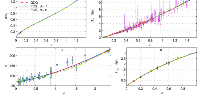
Predictions of different models in Fig. 1 are rather close, in particular, the curves for the models CDM and GCG practically coincide. The Hubble parameter in Fig. 1c is measured in km c-1Mpc-1, the distances and in Fig. 1b, d are in Gpc.
The data points for in Fig. 1d are calculated from in Table 5. Here the error boxes include the data spread between the recent estimations of the comoving sound horizon size:
| (36) |
III.1 CDM model
In the CDM model we use three free parameters , and in Eq. (16) for describing the considered observational data at . For the Hubble constant different approaches result in different estimations. In particular, observations of Cepheid variables in the project Hubble Space Telescope (HST) give the recent estimate km c-1Mpc-1 Riess11 . On the other hand, the satellite projects Planck Collaboration (Planck) Plank13 and Wilkinson Microwave Anisotropy Probe (WMAP) WMAP for observations of cosmic microwave background anisotropy result in the following values (in km c-1Mpc-1):
| (37) |
The nine-year results from WMAP WMAP include also the estimate km c-1Mpc-1 with added recent BAO and observations.
For the CDM model many authors WMAP ; Plank13 ; Tonry03 ; Knop03 ; Kowalski08 ; ShiHL12 ; FarooqMR13 ; FarooqR13 ; Farooqth calculated the best fits for parameters , and for describing the Type Ia supernovae, and BAO data in various combinations. In Refs. ShiHL12 ; FarooqMR13 ; FarooqR13 ; Farooqth some other cosmological models were compared with the CDM model. In particular, the authors ShiHL12 compared 8 models with two information criteria including minimal and the number of model parameters. Optimal values of these parameters were pointed out in Ref. ShiHL12 with the exception of , though is the important parameter for all 8 models.
In Refs. FarooqMR13 ; FarooqR13 ; Farooqth the CDM, XCDM and CDM models were applied to describe the supernovae, and BAO data. For all mentioned models the authors FarooqMR13 ; FarooqR13 ; Farooqth fixed two values of the Hubble constant GottV01 and km c-1Mpc-1 Riess11 and searched optimal values of other model parameters. But they did not estimated the best choice of among these two values and in the segment between them.
In this paper we pay the special attention to dependence of minima on . This dependence is very important if we compare different cosmological models.
The results of calculations WMAP ; Plank13 ; Kowalski08 ; ShiHL12 ; FarooqMR13 ; FarooqR13 ; Farooqth , as usual, are presented as level lines for the functions or of two parameters at (68.27%), (95.45%) and (99.73%) confidence levels. In particular, if a value is fixed, these two parameters for the CDM model may be and .
In Fig. 2 we use this scheme for 3 fixed values (37) indicated on the panels (including the optimal value km c-1Mpc-1) and draw level lines of the functions (29), (30), (34) and (35) in the plane and for with fixed in the bottom-right panel. The points of minima are marked in Fig. 2 as hexagrams for , pentagrams for , diamonds for and circles for . Minimal values of the functions (29), (30), (34) and (35) at these points are tabulated in Table 1 so we can compare efficiency of this description for different . For the same purpose we point out the corresponding values for some level lines in Fig. 2 and present the dependence of minima on and on in the left bottom panels of Fig. 2. Here we denote , and graphs of the fractions , , in are also shown.
In the bottom panels we present how parameters of a minimum point of depend on and on . In particular, for the dependence on the coordinates and of this point are calculated, the value is determined from Eq. (14). For the dependence on we also present the graph , where .
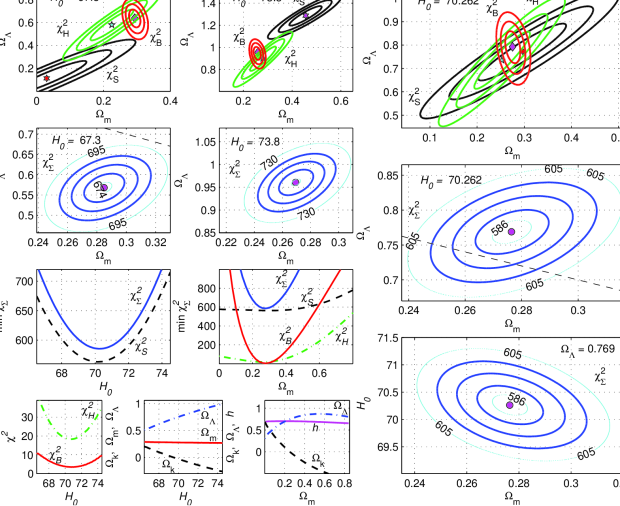
We see in Fig. 2 and in Table 1 that the dependence of is appreciable and significant. This function has the distinct minimum and achieves its minimal value at . The optimal values of the CDM model parameters , , corresponding to this minimum are presented in Table 2, these values are taken for the CDM curves in Fig. 1.
The mentioned sharp dependence of on is connected with two factors: (1) the similar dependence of the main contribution shown in the same panel; (2) the large shift of the minimum point for in the plane corresponding to growth. For and km c-1Mpc-1 this minimum point is far from the similar points of and . Only for close to 70 km c-1Mpc-1 all these three minimum points are near each other (the top-right panel in Fig. 2).
Only the value km c-1Mpc-1 in Table 1 is close to the optimal value in Table 2. We may conclude that the values of the Hubble constant and km c-1Mpc-1 taken in Refs. FarooqMR13 ; FarooqR13 ; Farooqth , unfortunately, lie to the left and to the right from the optimal value km c-1Mpc-1. We see the significant difference between the large values or for the too small and too large values of in Table 1 and the optimal value for in Table 2.
In the middle row panels of Fig. 2 with the flatness line (or ) is shown as the black dashed straight line. This line shows that only for close to the optimal value from Table 2 the following recent observational limitations on the CDM model parameters (13) from surveys WMAP ; Plank13
| (38) |
are satisfied on or level. For and km c-1Mpc-1 the optimal values of parameters , , in Table 1 are far from restrictions (38) for even on level.
| 67.3 | 599.37 | 18.492 | 5.548 | 673.64 | 0.285 | 0.568 | 0.147 |
| 69.7 | 562.73 | 17.993 | 3.517 | 588.53 | 0.278 | 0.734 | |
| 73.8 | 639.90 | 19.466 | 5.322 | 707.84 | 0.269 | 0.961 |
Graphs of the optimal values , and depending on are presented in the second bottom panel. We see that the value weakly depends on , but and satisfy conditions (38) only for km c-1Mpc-1.
The dependence of on is rather sharp because of the correspondent dependence of its fraction . This fact for is connected with the contribution from the value (32) measurements, because is proportional to and is very sensitive to values. Note that the fractions and (in ) weakly depend on .
Dependencies of on , and also , let us calculate estimates of acceptable values for these model parameters. They are presented below in Table 3.
Coordinates and of the minimum point for depend on in a such manner that only for values and satisfy conditions (38). Note that the optimal value of is close to 0.7 for all in the limits .
III.2 GCG model
Let us apply the model with generalized Chaplygin gas (GCG) KamenMP01 ; Bento02 ; Makler03 ; LuGX10 ; LiangXZ11 ; CamposFP12 ; XuLu12 to describing the same observational data for Type Ia supernovae, and BAO. We use here Eq. (18) with the initial condition , so we have 5 independent free parameters in this model: , , , and . However we really used only 4 free parameters, because the fraction may include not only baryonic but also a part of cold dark matter. Our calculations yield that the minimum over remaining 4 parameters practically does not depend on in the range (see Fig. 3). So in our analysis presented in Fig. 3 (except for 3 bottom-right panels) we fixed the value
that is the simple average of the WMAP WMAP and Planck Plank13 estimations.
In the GCG model and in accordance with Eq. (14) and the formal definition (13). However we should use the effective value in this model, in particular, in expression (32). In Refs. LuGX10 ; LiangXZ11 ; CamposFP12 ; XuLu12 ; LuXuWL11 the following effective value is used
| (39) |
This value results from correspondence between the models CDM with Eq. (16) and GCG with Eq. (18) in the early universe at .
But in our investigation the majority of observational data is connected with redshifts , so in Eq. (32) we are to consider the present time limit of the value . If we compare limits of the right hand sides of Eqs. (16) and (18) at or , we obtain another effective value
| (40) |
Values calculated with expressions (39) and (40) are different if . This difference looks like rather small if we compare minima of the sum (35) depending on . In Fig. 3 this dependence with Eq. (40) for is the blue solid line and for the case with Eq. (39) it is the violet dash-and-dot line. We see that the lines closely converge in the vicinity of the minimum point km c-1Mpc-1. The dependence in both cases (39) and (40) has the sharp minimum and resembles the case of the CDM model in Fig. 2. The value of this minimum, its parameters in Table 2, graph of the contribution and dependence on for parameters of the minimum point in the bottom-left panel in Fig. 3 are presented for the case with Eq. (40).
One should note that all mentioned dependencies are different for the case (39), in particular, the absolute minimum of is 584.31. This difference is illustrated in the central panels in Fig. 3 with level lines of for and 70.093 km c-1Mpc-1 (with the specified values , optimal for these ). These level lines are blue for the expression (40) and they are thin violet for Eq. (39). Positions of the optimal points are close only if is close to its optimal value in Table 2.
We suppose that the estimation of with the expression (40) is more adequate to the considered values . So in Table 2 and in other panels of Fig. 3 we use only Eq. (40). Notations in Fig. 3 correspond to Fig. 2.
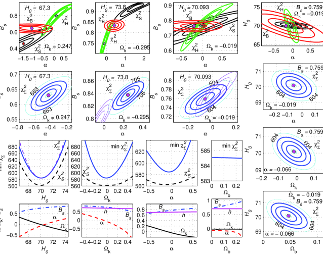
The similar dependence of on for the CDM and GCG models results in unsuccessful description of the data with and 73.8 km c-1Mpc-1 with the corresponding optimal values and . Fig. 3 illustrates large distances between minimum points of , and in these cases. The mentioned distances are small for the optimal values from Table 2 km c-1Mpc-1 and . For these optimal values we present level lines of in ; ; and planes. In these panels other model parameters are fixed and specified.
When we test dependence of the minimum on , , and in Fig. 3, we minimize this value over all other parameters (except for the above mentioned ). In particular, , this function has the distinct minimum near and resembles the dependence . The optimal value of or is practically constant and close to if we vary , or . As mentioned above the dependence of on is very weak, so we fixed in our previous analysis .
For the graph the correspondent minimum is achieved if is negative: (see Table 2). In the GCG model this parameter is connected with the square of adiabatic sound speed Makler03 ; CamposFP12 ; XuLu12
| (41) |
If we accept the restriction (equivalent to ) in our investigation with the mentioned observational data, we obtain the optimal value and the GCG model will be reduced to the CDM model with . The dependence of and other parameters on in Fig. 3 show that for we have and the optimal values of , , corresponding to the CDM model in Table 2.
| Model | other parameters | |||
|---|---|---|---|---|
| CDM | 585.35 | 70.262 | 0.276 | |
| GCG | 584.54 | 70.093 | 0.277 | |
| PCS, | 588.41 | 69.52 | 0.286 | |
| PCS, | 591.10 | 69.49 | 0.288 | |
| PCS, | 592.18 | 69.34 | 0.288 | |
| PCS, | 592.56 | 69.29 | 0.289 |
III.3 PCS model
The multidimensional gravitational model of I. Pahwa, D. Choudhury and T.R. Seshadri PahwaChS has the set of model parameters , , , , , similar to the GCG model, but also it has the additional integer-valued parameter (the number of extra dimensions). Our analysis demonstrated that the value is the most preferable for describing the observational data for supernovae, BAO and .
So it is the case that we present in almost all panels of Fig. 4 (except for 2 panels with dependencies of on and ). We use the similarity of model parameters for the GCG and PCS models draw in Fig. 4 the same graphs and level lines for the PCS model as in Fig. 3 in correspondent panels. Colors of correspondent lines also coincide. Naturally we use in Fig. 4 the value instead of .
The minimum (over all other parameters) increases when the baryon fraction grows. This dependence is more distinct than in the GCG case (Fig. 3), but it is also rather weak for small . So for the multidimensional model PCS we also fix and really use only 5 remaining parameters , , , , . The value is fixed in all panels of Fig. 4 like for Fig. 3 (except for 3 bottom-right panels).
The dependence of on has the distinct minimum at for (the solid blue line here and in panels of this row). The similar behavior takes place for (the violet dashed line) and for (the purple dots). The minimal value for is larger than for the CDM and GCG models and for the minima are still worse (see Table 2).
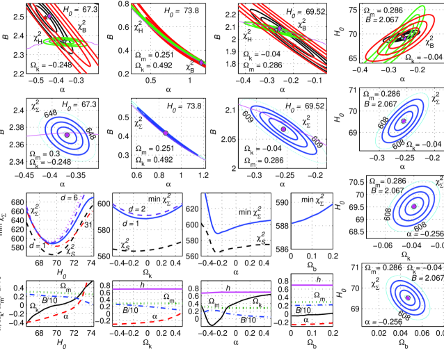
These bad results for the PCS model are connected with description of the recent data with high ( in Table 6). When we excluded 3 data points Busca12 ; Delubac14 ; Font-Ribera13 for with , we obtained absolutely other results presented below in Table 4.
In Fig. 4 all level lines and graphs correspond to the whole data with points. But only one except is done for the dependence of on for : here , this graph is shown as the red dash-and-dot line. The minimum value for this line is in Table 4.
Level lines of functions are shown in Fig. 4 in the same panels as for the GCG model in Fig. 3, in particular, for the values (37) , and the optimal value km c-1Mpc-1. If is too large, the domain of acceptable level of becomes very narrow. One should note that for all level lines we change only two parameters, all remaining model parameters are fixed (they are from Table 2 or optimal for a given ).
In 6 top-left panels with the plane we draw thin purple lines bounding the domain of regular solutions (below these lines). The upper domain (for larger ) consists of singular solutions, they have singularities in the past with infinite value of density corresponding to nonzero value of the scale factor GrSh13 . These solutions are nonphysical and should be excluded. It is interesting that the optimal solutions in Fig. 4 and in Tables 2 and 4 are near this border, but they are regular and describe the standard Big Bang with dynamical compactification of extra dimensions.
IV Conclusion
We considered how the CDM, GCG and PCS models describe the observational data for type Ia supernovae, BAO and SNTable , Tables 5, 6. These observations distinctly restrict acceptable values for the Hubble constant and other parameters of the mentioned models. We used our calculations for dependance , where the absolute minimum (over other parameters) of the value (35) depend on a fixed parameter . On the base of these calculations (presented partially in Figs. 2, 3, 4) we obtained the following estimates for parameters of the CDM, GCG and PCS () models:
| Model | other parameters | |||
|---|---|---|---|---|
| CDM | 585.35 | == | ||
| GCG | 584.54 | = | ||
| PCS, | 588.41 | = |
Our estimates for the CDM model are in agreement with the WMAP observational restrictions (38) on , , WMAP , but they are in tension with the Planck data Plank13 . This fact is connected with too low value km c-1Mpc-1 (37) in the Planck survey Plank13 .
For the GCG model is slightly better and our limitations on and in Table 3 are rather close to the CDM case. However, if we require in accordance with Eq. (41) and Refs. CamposFP12 ; XuLu12 , the GCG model with the optimal value will be reduced to the CDM model with its optimal parameters in Tables 2, 3 and the same .
Values and for the GCG model essentially depend on the expression for (39) or (40). But the optimal parameters in Table 2 for these expressions are rather close.
We mentioned above that the multidimensional model PCS is less effective in description of the considered observational data, and that the main problem of this model is connected with the recent data with high (). We excluded 3 data points Busca12 ; Delubac14 ; Font-Ribera13 with , 2.34, 2.36 and for remaining points of and the same SN and BAO data from SNTable , Table 5. we calculated and optimal values of model parameters presented here in Table 4.
| Model | other parameters | |||
|---|---|---|---|---|
| CDM | 583.71 | 70.12 | 0.281 | |
| GCG | 583.70 | 70.11 | 0.291 | |
| PCS, | 582.68 | 69.89 | 0.281 | |
| PCS, | 582.93 | 69.82 | 0.282 | |
| PCS, | 583.23 | 69.78 | 0.282 |
We see that the model PCS PahwaChS describes the reduced set of data with better than other models. The best fit is for , the optimal value of close to km c-1Mpc-1.
This example demonstrates that predictions of any cosmological model essentially depend on data selection. Moreover, there is the important problem of model dependence (in addition to mutual dependence) of observational data, in particular, data in Tables 5, 6.
Leaving the last problem beyond this paper, we can conclude that the considered observations of type Ia supernovae SNTable , BAO (Table 5) and the Hubble parameter (Table 6) confirm effectiveness of the CDM model, but they do not deny other models. The important argument in favor of the CDM model is its small number of model parameters (degrees of freedom). This number is part of information criteria of model selection statistics, in particular, the Akaike information criterion is ShiHL12 . This criterion supports the leading position of the CDM model.
Appendix A Appendix
| Refs | |||||
|---|---|---|---|---|---|
| 0.106 | 0.336 | 0.015 | 0.526 | 0.028 | WMAP |
| 0.20 | 0.1905 | 0.0061 | 0.488 | 0.016 | WMAP |
| 0.35 | 0.1097 | 0.0036 | 0.484 | 0.016 | WMAP |
| 0.44 | 0.0916 | 0.0071 | 0.474 | 0.034 | BlakeBAO11 |
| 0.57 | 0.07315 | 0.0012 | 0.436 | 0.017 | WMAP ; Chuang13 |
| 0.60 | 0.0726 | 0.0034 | 0.442 | 0.020 | BlakeBAO11 |
| 0.73 | 0.0592 | 0.0032 | 0.424 | 0.021 | BlakeBAO11 |
Measurements of and in Ref. BlakeBAO11 are not independent, they are described with the following elements of covariance matrices and in Eq. (34) WMAP ; BlakeBAO11 :
These matrices are symmetric ones, their remaining elements are , , .
| Refs | Refs | ||||||
| 0.070 | 69 | 19.6 | Zhang12 | 0.57 | 92.9 | 7.855 | Anderson13 |
| 0.090 | 69 | 12 | Simon05 | 0.593 | 104 | 13 | Moresco12 |
| 0.120 | 68.6 | 26.2 | Zhang12 | 0.600 | 87.9 | 6.1 | Blake12 |
| 0.170 | 83 | 8 | Simon05 | 0.680 | 92 | 8; | Moresco12 |
| 0.179 | 75 | 4 | Moresco12 | 0.730 | 97.3 | 7.0 | Blake12 |
| 0.199 | 75 | 5 | Moresco12 | 0.781 | 105 | 12 | Moresco12 |
| 0.200 | 72.9 | 29.6 | Zhang12 | 0.875 | 125 | 17 | Moresco12 |
| 0.240 | 79.69 | 2.65 | Gazta09 | 0.880 | 90 | 40 | Stern10 |
| 0.270 | 77 | 14 | Simon05 | 0.900 | 117 | 23 | Simon05 |
| 0.280 | 88.8 | 36.6 | Zhang12 | 1.037 | 154 | 20 | Moresco12 |
| 0.300 | 81.7 | 6.22 | Oka13 | 1.300 | 168 | 17 | Simon05 |
| 0.350 | 82.7 | 8.4 | Chuang12 | 1.430 | 177 | 18 | Simon05 |
| 0.352 | 83 | 14 | Moresco12 | 1.530 | 140 | 14 | Simon05 |
| 0.400 | 95 | 17 | Simon05 | 1.750 | 202 | 40 | Simon05 |
| 0.430 | 86.45 | 3.68 | Gazta09 | 2.300 | 224 | 8 | Busca12 |
| 0.440 | 82.6 | 7.8 | Blake12 | 2.340 | 222 | 7 | Delubac14 |
| 0.480 | 97 | 62 | Stern10 | 2.360 | 226 | 8 | Font-Ribera13 |
Acknowledgements.
G.S. would like to acknowledge the support of the Ministry of education and science of Russia (grant No. 1.476.2011).References
- (1) A.G. Riess et al., Observational Evidence from Supernovae for an Accelerating Universe and a Cosmological Constant, Astron. J. 116 (1998) 1009 [astro-ph/9805201].
- (2) S. Perlmutter et al., Measurements of Omega and Lambda from 42 high redshift supernovae, Astrophys. J. 517 (1999) 565 [astro-ph/9812133].
- (3) N. Suzuki et al., The Hubble Space Telescope Cluster Supernova Survey: V. Improving the Dark Energy Constraints Above z¿1 and Building an Early-Type-Hosted Supernova Sample, Astrophys. J. 746 (2012) 85 [arXiv:1105.3470].
- (4) D.H. Weinberg et al., Observational Probes of Cosmic Acceleration, Physics Reports 530 (2013) 87 [arXiv:1201.2434].
- (5) G. Hinshaw et al., Nine-year Wilkinson Microwave Anisotropy Probe (WMAP) Observations: Cosmological Parameters Results, Astrophysical Journal Suppl. 208 (2013) 19 [arXiv:1212.5226].
- (6) D.J. Eisenstein et al., Detection of the baryon acoustic peak in the large-scale correlation function of SDSS luminous red galaxies, Astrophys. J. 633(2) (2005) 560 [astro-ph/0501171].
- (7) B.A. Reid et al., Cosmological constraints from the clustering of the Sloan Digital Sky Survey DR7 luminous red galaxies, Mon. Not. Roy. Astron. Soc. 404 (2010) 60 [arXiv:0907.1659].
- (8) P.A.R. Ade et al., Planck 2013 results. XVI. Cosmological parameters, arXiv:1303.5076.
- (9) J. Simon, L. Verde and R. Jimenez, Constraints on the redshift dependence of the dark energy potential, Phys. Rev. D 71 (2005) 123001 [astro-ph/0412269].
- (10) D. Stern, R. Jimenez, L. Verde, M. Kamionkowski and S. A. Stanford, Cosmic chronometers: constraining the equation of state of dark energy. I: measurements, J. of Cosmology and Astropart. Phys. 02 (2010) 008 [arXiv:0907.3149].
- (11) M. Moresco et al., Improved constraints on the expansion rate of the Universe up to 1.1 from the spectroscopic evolution of cosmic chronometers, J. of Cosmology and Astropart. Phys. 8 (2012) 006 [arXiv:1201.3609].
- (12) C. Blake et al., The WiggleZ Dark Energy Survey: Joint measurements of the expansion and growth history at , Mon. Not. Roy. Astron. Soc. 425(1) (2012) 405 [arXiv:1204.3674].
- (13) C. Zhang et al., Four New Observational H(z) Data From Luminous Red Galaxies Sloan Digital Sky Survey Data Release Seven, arXiv:1207.4541.
- (14) N.G. Busca et al., Baryon Acoustic Oscillations in the Ly forest of BOSS quasars, Astron. and Astrop. 552 (2013) A96 [arXiv:1211.2616].
- (15) C.H. Chuang and Y. Wang, Modeling the Anisotropic Two-Point Galaxy Correlation Function on Small Scales and Improved Measurements of , , and from the Sloan Digital Sky Survey DR7 Luminous Red Galaxies, Mon. Not. Roy. Astron. Soc. 435(1) (2013) 255 [arXiv:1209.0210].
- (16) E. Gaztañaga, A. Cabre, L. Hui, Clustering of Luminous Red Galaxies IV: Baryon Acoustic Peak in the Line-of-Sight Direction and a Direct Measurement of , Mon. Not. Roy. Astron. Soc. 399(3) (2009) 1663 [arXiv:0807.3551].
- (17) L. Anderson et al., The clustering of galaxies in the SDSS-III Baryon Oscillation Spectroscopic Survey: Measuring and at from the Baryon Acoustic Peak in the Data Release 9 Spectroscopic Galaxy Sample, Mon. Not. Roy. Astron. Soc. 439(1) (2014) 83 [arXiv:1303.4666].
- (18) A. Oka et al., Simultaneous constraints on the growth of structure and cosmic expansion from the multipole power spectra of the SDSS DR7 LRG sample, Mon. Not. Roy. Astron. Soc. 439(3) (2014) 2515 [arXiv:1310.2820].
- (19) T. Delubac et al., Baryon Acoustic Oscillations in the Ly forest of BOSS DR11 quasars, arXiv:1404.1801.
- (20) A. Font-Ribera et al., Quasar-Lyman Forest Cross-Correlation from BOSS DR11: Baryon Acoustic Oscillations, J. of Cosmology and Astroparticle Phys. 05 (2014) 027 [arXiv:1311.1767].
- (21) C. Blake et al., The WiggleZ dark energy survey: mapping the distance redshift relation with baryon acoustic oscillations, Mon. Not. Roy. Astron. Soc. 418(3) (2011) 1707 [arXiv:1108.2635].
- (22) C-H. Chuang et al., The clustering of galaxies in the SDSS-III Baryon Oscillation Spectroscopic Survey: single-probe measurements and the strong power of on constraining dark energy, Mon. Not. Roy. Astron. Soc. 433(4) (2013) 3559 [arXiv:1303.4486].
- (23) T. Clifton, P.G. Ferreira, A. Padilla and C. Skordis, Modified Gravity and Cosmology, Physics Reports 513 (2012) 1 [arXiv:1106.2476].
- (24) K. Bamba, S. Capozziello, S. Nojiri and S.D. Odintsov, Dark energy cosmology: the equivalent description via different theoretical models and cosmography tests, Astrophys. and Space Science 342 (2012) 155 [arXiv:1205.3421].
- (25) E.J. Copeland, M. Sami and S. Tsujikawa, Dynamics of dark energy, Int. J. Mod. Phys. D 15 (2006) 1753 [hep-th/0603057].
- (26) M. Kunz, The phenomenological approach to modeling the dark energy, Comptes rendus - Physique 13 (2012) 539, [arXiv:1204.5482].
- (27) T.P. Sotiriou and V. Faraoni, f(R) theories of gravity, Rev. of Modern Phys. 82 (2010) 451 [arXiv:0805.1726].
- (28) S. Nojiri and S. D. Odintsov, Unified cosmic history in modified gravity: from F(R) theory to Lorentz non-invariant models, Phys. Rept. 505 (2011) 59 [arxiv:1011.0544].
- (29) R. R. Caldwell, R. Dave and P. J. Steinhardt, Cosmological imprint of an energy component with general equation of state, Phys. Rev. Lett. 80 (1998) 1582 [astro-ph/9708069].
- (30) J. Khoury and A. Weltman, Chameleon cosmology, Phys. Rev. D 69 (2004) 044026 [astro-ph/0309411].
- (31) A.Y. Kamenshchik, U. Moschella and V. Pasquier An alternative to quintessence, Phys. Lett. B 511(2-4) (2001) 265 [arXiv:gr-qc/0103004].
- (32) M.C. Bento, O. Bertolami and A.A. Sen, Generalized Chaplygin gas, accelerated expansion, and dark-energy-matter unification, Phys. Rev. D 66(4) (2002) 043507 [arXiv:gr-qc/0202064].
- (33) M. Makler, S.Q. de Oliveira and I. Waga, Constraints on the generalized Chaplygin gas from supernovae observations, Phys. Lett. B 555(1-2) (2003) 1 [arXiv:astro-ph/0209486].
- (34) J. Lu, Y. Gui and L. Xu, Observational constraint on generalized Chaplygin gas model, Eur. Phys. J. C. 63 (2009) 349 [arXiv:1004.3365].
- (35) N. Liang, L. Xu and Z. Zhu, Constraints on the generalized Chaplygin gas model including gamma-ray bursts via a Markov Chain Monte Carlo approach, Astron. Astrophys. 527 (2011) A11 [arXiv:1009.6059].
- (36) J.P. Campos, J.C. Fabris, R. Perez, O.F. Piattella and H. Velten, Does Chaplygin gas have salvation? Eur. Phys. J. C. 73 (2013) 2357 [arXiv:1212.4136].
- (37) L. Xu, J. Lu and Y. Wang, Revisiting Generalized Chaplygin Gas as a Unified Dark Matter and Dark Energy Model, Eur. Phys. J. C. 72 (2012) 1883 [arXiv:1204.4798].
- (38) J. Lu, L. Xu, Y. Wu, and M. Liu, Combined constraints on modified Chaplygin gas model from cosmological observed data: Markov Chain Monte Carlo approach, Gen. Rel. Grav. 43 (2011) 819 [arXiv:1105.1870].
- (39) B.C. Paul and P. Thakur, Observational constraints on modified Chaplygin gas from cosmic growth, J. of Cosmology and Astropart. Phys. 11 (2013) 052 [arXiv:1306.4808].
- (40) N. Mohammedi, Dynamical Compactification, Standard Cosmology and the Accelerating Universe, Phys. Rev.D 65 (2002) 104018 [hep-th/0202119].
- (41) F. Darabi, Accelerating Universe and Dynamical Compactification of Extra Dimensions, Class. Quant. Grav. 20 (2003) 3385 [gr-qc/0301075].
- (42) T. Bringmann, M. Eriksson and M. Gustafsson, Cosmological Evolution of Homogeneous Universal Extra Dimensions, Phys. Rev. D 68 (2003) 063516 [astro-ph/0303497].
- (43) D. Panigrahi, Y.Z. Zhang and S. Chatterjee, Accelerating Universe as Window for Extra Dimensions, Int. J. Mod. Phys. A 21 (2006) 6491 [gr-qc/0604079].
- (44) C. A. Middleton and E. Stanley, Anisotropic evolution of 5D Friedmann-Robertson-Walker spacetime, Phys. Rev. D 84 (2011) 085013 [arXiv:1107.1828].
- (45) H. Farajollahi and H. Amiri, 5D noncompact Kaluza -Klein cosmology in the presence of Null perfect fluid, Int. J. Mod. Phys. D 19 (2010) 1823 [arXiv:1005.3140].
- (46) I. Pahwa, D. Choudhury and T. R. Seshadri, Late-time acceleration in Higher Dimensional Cosmology, J. of Cosmology and Astroparticle Phys. 09 (2011) 015 [arXiv:1104.1925].
- (47) O.A. Grigorieva and G.S. Sharov, Multidimensional gravitational model with anisotropic pressure, Intern. Journal of Modern Physics D 22 (2013) 1350075 [arXiv:1211.4992].
- (48) A.G. Riess et al., A 3% Solution: Determination of the Hubble Constant with the Hubble Space Telescope and Wide Field Camera 3, Astrophys. J. 730(2) (2011) 119 [arXiv:1103.2976].
- (49) et al. 2003, ApJ, 594, 1 J.L. Tonry et al., Cosmological Results from High-z Supernovae, Astrophys. J. 594 (2003) 1, arXiv:astro-ph/0305008
- (50) . R.A. Knop et al., New Constraints on , , and from an Independent Set of Eleven High-Redshift Supernovae Observed with HST1, Astrophys. J. 598 (2003) 102, arXiv:astro-ph/0309368.
- (51) M. Kowalski et al., Improved cosmological constraints from new, old and combined supernova datasets, Astrophys. J. 686 (2008) 749 [arXiv:0804.4142].
- (52) K. Shi, Y.F. Huang and T. Lu, A comprehensive comparison of cosmological models from the latest observational data, Monthly Notices Roy. Astronom. Soc. 426 (2012) 2452 [arXiv:1207.5875].
- (53) O. Farooq, D. Mania and B. Ratra, Hubble parameter measurement constraints on dark energy, Astrophys. J. 764 (2013) 139 [arXiv:1211.4253].
- (54) O. Farooq and B. Ratra, Hubble parameter measurement constraints on the cosmological deceleration-acceleration transition redshift, Astrophys. J. 766 (2013) L7, [arXiv:1301.5243].
- (55) O. Farooq, Ph.D. thesis, arXiv:1309.3710.
- (56) J.R. Gott III, M.S. Vogeley, S. Podariu and B. Ratra, Median statistics, h0, and the accelerating universe, Astrophys. J. 549 (2001) 1.