Conditional entropy of ordinal patterns
Abstract
In this paper we investigate a quantity called conditional entropy of ordinal patterns, akin to the permutation entropy.
The conditional entropy of ordinal patterns describes the average diversity of the ordinal patterns succeeding a given ordinal pattern.
We observe that this quantity provides a good estimation of the Kolmogorov-Sinai entropy in many cases.
In particular, the conditional entropy of ordinal patterns of a finite order coincides with the Kolmogorov-Sinai entropy for periodic dynamics and for Markov shifts over a binary alphabet.
Finally, the conditional entropy of ordinal patterns is computationally simple and thus can be well applied to real-world data.
Keywords: Conditional entropy; Ordinal pattern; Kolmogorov-Sinai entropy; Permutation entropy; Markov shift; Complexity.
1 Introduction
The question how can one quantify the complexity of a system often arises in various fields of research. On the one hand, theoretical measures of complexity like the Kolmogorov-Sinai (KS) entropy [2, 1], the Lyapunov exponent [1] and others are not easy to estimate from given data. On the other hand, empirical measures of complexity often lack of a theoretical foundation, see for instance the discussion of the renormalized entropy and its relationship to the Kullback-Leibler entropy in [3, 4, 5, 6]. Sometimes they are also not well interpretable, for example, see [7] for a criticism of the approximate entropy interpretability.
One of possible approaches to measuring complexity is based on ordinal pattern analysis [8, 10, 9]. In particular, the permutation entropy of some order can easily be estimated from the data and has a theoretical counterpart (for order tending to infinity), which is a justified measure of complexity. However, in this paper we consider another ordinal-based quantity, the conditional entropy of ordinal patterns. We show that for a finite order in many cases it is closer to the KS entropy than the permutation entropy.
The idea behind ordinal pattern analysis is to consider order relations between values of time series instead of the values themselves. The original time series is converted to a sequence of ordinal patterns of an order , each of them describing order relations between successive points of the time series, as demonstrated in Figure 1 for order .
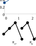
The more complex the underlying dynamical system is, the more diverse the ordinal patterns occurring for the time-series are. This diversity is just what the permutation entropy measures. For example, in Figure 1 the permutation entropy of order is equal to , since there are four different ordinal patterns occurring with the same frequency. The permutation entropy is robust to noise [9], computationally simple and fast [10]. For order tending to infinity the permutation entropy is connected to the central theoretical measure of complexity for dynamical systems: it is equal to the KS entropy in the important particular case [11], and it is not lower than the KS entropy in a more general case [12].
However, the permutation entropy of finite order does not estimate the KS entropy well, while being an interesting practical measure of complexity. Even if the permutation entropy converges to the KS entropy as order tends to infinity, the permutation entropy of finite can be either much higher or much lower than the KS entropy (see Subsection 3.5 for details).
Therefore we propose to consider the conditional entropy of ordinal patterns of order : as we demonstrate, in many cases it provides a much better practical estimation of the KS entropy than the permutation entropy, while having the same computational efficiency. The conditional entropy of ordinal patterns characterizes the average diversity of ordinal patterns succeeding a given one. For the example in Figure 1 the conditional entropy of ordinal patterns of order is equal to zero since for each ordinal pattern only one successive ordinal pattern occurs ( is the only successive ordinal pattern for , is the only successive ordinal pattern for and so on).
Let us motivate the discussion of the conditional entropy of ordinal patterns by an example.
Example 1.
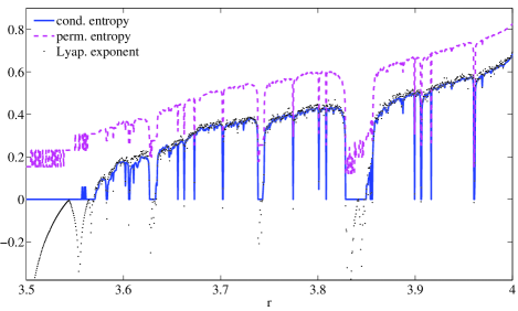
Consider the family of logistic maps defined by . For almost all the KS entropy either coincides with the Lyapunov exponent if it is positive or is equal to zero otherwise (this holds by Pesin’s formula [13, Theorems 4, 6], due to the properties of -invariant measures [14]). Note that the Lyapunov exponent for the logistic map can be estimated rather accurately [15]. For the logistic maps the permutation entropy of order converges to the KS entropy as tends to infinity. However, Figure 2 shows that for the permutation entropy of order is relatively far from the Lyapunov exponent in comparison with the conditional entropy of ordinal patterns of the same order (values of both entropies are numerically estimated from orbits of length of a ‘random point’ in ).
In this paper we demonstrate that under certain assumptions the conditional entropy of ordinal patterns estimates the KS entropy better than the permutation entropy (Theorem 1). Besides, we prove that for some dynamical systems the conditional entropy of ordinal patterns for a finite order coincides with the KS entropy (Theorems 5, 6), while the permutation entropy only asymptotically approaches the KS entropy.
The paper is organized as follows. In Section 2 we fix the notation, recall the definition of the KS entropy and basic notions from ordinal pattern analysis. In Section 3 we introduce the conditional entropy of ordinal patterns and show that in some cases it approaches the KS entropy faster than the permutation entropy. Moreover, we prove that the conditional entropy of ordinal patterns for finite order coincides with the KS entropy for Markov shifts over two symbols (Subsection 3.3) and for systems with periodic dynamics (Subsection 3.4). In Section 4 we consider the interrelation between the conditional entropy of ordinal patterns, the permutation entropy and the sorting entropy [8]. In Section 5 we observe some open question and make a conclusion. Finally, in Section 6 we provide those proofs that are mainly technical.
2 Preliminaries
2.1 Kolmogorov-Sinai entropy
In this subsection we recall the definition of the KS entropy of a dynamical system and define some related notions we will use further on. Throughout the paper we use the same notation as in [16] and refer to this paper for a brief introduction. For a general discussion and details we refer the reader to [1, 17].
We focus on a measure-preserving dynamical system , where is a non-empty topological space, is the Borel sigma-algebra on it, is a probability measure, and is a --measurable -preserving map, i.e. for all .
The complexity of a system can be measured by considering a coarse-grained description of it provided by symbolic dynamics. Given a finite partition of (below we consider only partitions without mentioning this explicitly), one assigns to each set the symbol from the alphabet . Similarly, the -letter word is associated with the set defined by
| (1) |
Then the collection
| (2) |
forms a partition of as well. The Shannon entropy, the entropy rate and the Kolmogorov-Sinai (KS) entropy are respectively defined by (we use the convention that )
The latter quantity provides a theoretical measure of complexity for a dynamical system. In general, the determination of the KS entropy is complicated, thus the estimation of the KS entropy (from real-world data as well) is of interest.
2.2 Ordinal patterns, permutation entropy and sorting entropy
Let us first recall the definitions of ordinal patterns and ordinal partitions. For denote the set of permutations of by .
Definition 1.
We say that a real vector has the ordinal pattern of order if
and
Definition 2.
For , let be an -valued random vector on . Then for the partition
with
is called the ordinal partition of order with respect to and .
The permutation entropy of order (with respect to ) and the sorting entropy of order (with respect to ), being ordinal-based complexity measures for time series, are respectively given by
(note that the original definitions in [8] were given for the case and , where is the identity map). The permutation entropy is often defined just as , but for us it is more convenient to use the definition above. The sorting entropy represents the increase of diversity of ordinal patterns as the order increases by one. To see the physical meaning of the permutation entropy let us rewrite it in the explicit form. Given , we have
that is the permutation entropy characterizes the diversity of ordinal patterns divided by the order .
In applications permutation and sorting entropy of order can be estimated from a finite orbit of a dynamical system with certain properties. Simple and natural estimators are the empirical permutation entropy and the empirical sorting entropy, respectively. They are based on estimating by the empirical probabilities of observing in the time series generated by .
Finally, recall that the permutation and sorting entropy are related to the KS entropy. For the case , being a piecewise strictly-monotone interval map and , Bandt et al. [11] proved that:
Keller and Sinn [18, 19, 12] showed that in many cases (see [20] for recent results) it holds:
| (3) |
Note that if (3) holds, then the permutation entropy and the sorting entropy for tending to infinity provide upper bounds for the KS entropy [12]:
One may ask whether it is possible to get a better ordinal-based estimator of the KS entropy using the representation (3). This question is discussed in the next section.
3 Conditional entropy of ordinal patterns and its relation to the Kolmogorov-Sinai entropy
The conditional entropy of ordinal patterns of order is defined by
| (4) |
It is the first element of the sequence
which provides the ordinal representation (3) of the KS entropy as both and tend to infinity. For brevity we refer to as the ‘conditional entropy’ when no confusion can arise.
To see the physical meaning of the conditional entropy recall that the entropies of the partitions and are given by
Then we can rewrite the conditional entropy (4) as
If for some with and , then we say that in the ordinal patterns are successors of the ordinal patterns , respectively. The conditional entropy characterizes the diversity of successors of given ordinal patterns , whereas the permutation entropy characterizes the diversity of ordinal patterns themselves.
In the rest of the section we discuss the relationship between the conditional entropy of ordinal patterns and the KS entropy.
3.1 Relationship in the general case
Statements (i) and (ii) of the following theorem imply that under the given assumptions the conditional entropy of ordinal patterns bounds the KS entropy better than the sorting entropy and the permutation entropy, respectively.
Theorem 1.
Let be a measure-preserving dynamical system, be a random vector on such that (3) is satisfied. Then it holds
| (5) |
| or the limit of the sorting entropy |
| (6) |
| then it holds: |
| (7) |
The proof is given in Subsection 6.1. Note that both statements of Theorem 1 remain correct if one replaces the upper limits by the lower limits.
As a consequence of Theorem 1 we get the following result.
Corollary 2.
This sheds some light on the behavior of the conditional entropy for the logistic maps, described in Example 1. Nevertheless, it is not clear whether the statements (5) or (6) hold, neither in the general case nor for the logistic maps. Note that a sufficient condition for (6) is the monotone decrease of the sorting entropy with increasing . However, the sorting entropy and the permutation entropy do not necessarily decrease for all .
Example 2.
Consider the golden mean map defined by
for being the golden ratio. The map preserves the measure [1] given by for all and for
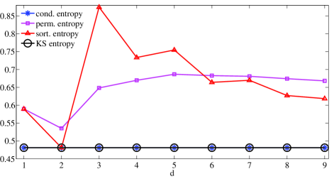
The values of permutation, sorting and conditional entropies for the dynamical system estimated from the orbit of length are shown in Figure 3. Note that neither sorting nor permutation entropy is monotonically decreasing with increasing . (The interesting fact that for all the conditional entropy and the KS entropy coincide is explained in Subsection 3.3.)
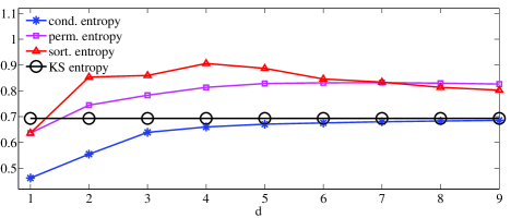
The question when or decrease starting from some is still open. For instance, for the logistic map with our estimated values of permutation entropy and sorting entropy decrease starting from and , respectively (see Figure 4). However, at this point we do not have theoretical results in this direction.
3.2 Markov property of ordinal partition
Computation of the KS entropy involves taking a supremum over all finite partitions and is unfeasible in the general case. A possible solution is provided by the properties given in Definitions 3 and 4.
Definition 3.
A finite partition of is said to be generating (under ) if, given the sigma-algebra generated by the sets with and , for every there exists a set such that .
Definition 4.
A finite partition of has the Markov property with respect to and if for all with and it holds
| (8) |
Originally in [21] a partition with property (8) was called Markov partition, but we use another term to avoid confusion with the topological notion of Markov partition.
By the Kolmogorov-Sinai theorem (for details we refer to [2, Theorem 4.17]), if is a generating partition then it holds . Further, it is easy to show (see [17, Observation 6.2.10]) that for the partition with the Markov property it holds
Therefore, if is both generating and has the Markov property, then
From the last two statements it follows the sufficient condition for the coincidence between the conditional entropy and the KS entropy.
Lemma 3.
Let be a measure-preserving dynamical system, be an -valued random vector on such that (3) is satisfied. Then the following two statements hold:
-
(i)If has the Markov property for all then
(ii)If is generating and has the Markov property for some then
(9)
In general, it is complicated to verify that ordinal partitions are generating or have the Markov property; however in Subsection 3.3 this is done for Markov shifts over two symbols.
3.3 Markov shifts
In this subsection we establish the equality of the conditional entropy of order and the KS entropy for the case of Markov shifts over two symbols. First we recall the definition of the Markov shifts (see [17, Section 6] for details), then we impose a natural restriction on the observables, state the result and finally discuss some possible extensions.
Definition 5.
Let be an stochastic matrix and be a stationary probability vector of with . Then a Markov shift is the dynamical system , where
-
•
is the space of one-sided sequences over ,
-
•
is the Borel sigma-algebra generated by the cylinder sets given by
-
•
such that for all and is a shift map,
-
•
is a Markov measure on , defined on the cylinder sets by
In the particular case when for all , the measure defined as follows is said to be a Bernoulli measure:
The system is then called a Bernoulli shift. We use this concept below for illustration purposes.
The natural order on the set of sequences is the lexicographic order defined as follows: for the inequality holds iff or there exists some with for and . However, we prefer to be consistent in using the concept of ordinal patterns and to keep working with the usual order on observables instead of considering particular orders on different spaces. Thus, to introduce the ordinal partition for Markov shifts, we impose a restriction on the observables on .
Definition 6.
Let us say that the observable is lexicographic-like if for almost all it is injective and if for all and the inequality holds iff .
In other words, the fact that an observable is lexicographic-like means that an induces the natural order relation on . A simple example of such is provided by considering as -expansions of a number in :
Note that since a lexicographic-like is injective for almost all , it provides the ordinal representation (3) of the KS entropy (see [12]).
Recall that the dynamical system is ergodic if for every with it holds either or . In Subsection 6.4 we prove the following statement.
Lemma 4.
Let be an ergodic Markov shift over two symbols. If the random variable is lexicographic-like, then the ordinal partition is generating and has the Markov property for all .
Theorem 5.
Under the assumptions of Lemma 4 for all it holds
Example 3.
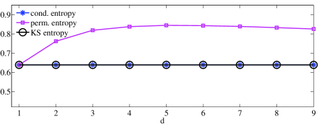
Figure 5 illustrates Theorem 5 for the Bernoulli shift over two symbols with , . For all the empirical conditional entropy computed from an orbit of length nearly coincides with the theoretical KS entropy . Meanwhile, the empirical permutation entropy differs from the KS entropy significantly.
The result established in Theorem 5 naturally extends to the class of maps that are order-isomorphic to an ergodic Markov shift over two symbols (the concept of order-isomorphism is introduced in [9]). An example of a map being order-isomorphic to a Markov shift is the golden mean map considered in Example 2. It explains the coincidence of the conditional entropy and the KS entropy in Figure 3. Note that the logistic map for is isomorphic, but not order-isomorphic to an ergodic Markov shift over two symbols [9, Subsection 3.4.1]. Therefore in the case of the logistic map with the conditional entropy for finite does not coincide with the KS entropy (see Figure 4).
Theorem 5 cannot be extended to Markov shifts over a general alphabet. One can rigorously show that for the Bernoulli shifts over more than two symbols, does not have the Markov property.
Example 4.
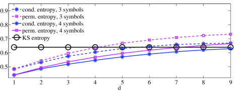
Figure 6 represents estimated values of the empirical conditional and permutation entropies for the Bernoulli shifts over three and four symbols. Although these shifts have the same KS entropy as the shift in Figure 5, their conditional entropies differ significantly.
3.4 Periodic case
Here we relate the conditional entropy to the KS entropy in the case of periodic dynamics. By periodic dynamical system we mean a system such that the set of periodic points has measure . Though it is well known that the KS entropy of a periodic dynamical system is equal to zero, the permutation entropy of order can be arbitrarily large in this case and thus does not provide a reliable estimate for the KS entropy. In Theorem 6 we show that the conditional entropy of a periodic dynamical system is equal to the KS entropy starting from some finite order , which advantages the conditional entropy over the permutation entropy.
Theorem 6.
Let be a measure-preserving dynamical system. Suppose that the set of periodic points of with period not exceeding has measure , then for all with it holds
The proof is given in Subsection 6.2.
Example 5.
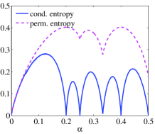
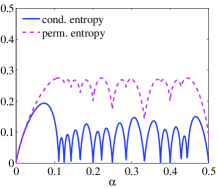
In order to illustrate the behavior of permutation and conditional entropies of periodic dynamical systems, consider the rotation maps on the interval with the Lebesgue measure . Let be rational, then provides a periodic behavior and it holds . Figure 7 illustrates conditional and permutation entropies for the rotation maps for and for varying with step 0.001. For both values of the conditional entropy is more close to zero than the permutation entropy since periodic orbits provide various ordinal patterns, but most of them have one and the same successor. Note that for those values of forcing periods shorter than (for instance for all have period ) it holds as provided by Theorem 6.
(a)
(b)
3.5 Relationship between permutation entropy and Kolmogorov-Sinai entropy
We finish this section by giving several reasons for why the permutation entropy of finite does not provide an appropriate estimation of the KS entropy (even if ). First, the permutation entropy of order converges to rather slowly [11]. Second, the permutation entropy of order is bounded from above, which means that for a relatively small a relatively large KS entropy cannot be correctly estimated. Indeed, given an -valued random vector on , for all it holds
| (10) |
To see this recall that there are different ordinal patterns of order . Therefore by general properties of the Shannon entropy we have
and inequality (10) becomes obvious.
Finally, as we have already mentioned in Subsection 3.4, the permutation entropy of order can be arbitrarily large for simple systems. In particular, for any given one can construct a periodic dynamical system such that the permutation entropy of order reaches the maximal possible value provided by inequality (10), while .
Example 6.
Consider a map , defined as follows
on the interval with the Lebesgue measure . All points are periodic with period , as one can easily check, therefore . However, all ordinal patterns of order occur with equal frequency , which provides for (cf. (10)).
4 Interrelationship between conditional entropy of ordinal patterns, permutation and sorting entropy
In this section we consider the relationship between the conditional entropy of order , the permutation entropy and the sorting entropy . Besides being interesting in its own right, this relationship is used to prove Theorem 1.
Lemma 7.
Let be a measure-preserving dynamical system. Then for all it holds
| (11) |
Moreover, if for some it holds , then we get
| (12) |
Proof.
By Lemma 7 we have that the conditional entropy under certain assumption is not greater than the permutation entropy and that in the general case the conditional entropy is not greater than the sorting entropy. Moreover, one can show that in the strong-mixing case the conditional entropy and the sorting entropy asymptotically approach each other. To see this recall that the map is said to be strong-mixing if for every it holds
According to [22], if is an interval in and is strong-mixing then it holds
Together with Lemma 7 this implies the following statement.
Corollary 8.
Let be a measure-preserving dynamical system, where is an interval in and is strong-mixing. Then
5 Conclusions
As we have discussed, the conditional entropy of ordinal patterns has rather good properties. Our theoretical results and numerical experiments show that in many cases the conditional entropy provides a reliable estimation of the KS entropy. In this regard it is important to note that the conditional entropy is computationally simple: it has the same computational complexity as the permutation entropy. (The algorithm for fast computing the conditional entropy of ordinal patterns, based on ideas presented in [23], will be discussed elsewhere.)
Meanwhile, some questions concerning the conditional entropy of ordinal patterns remain open. In particular, possible directions of a future work are to find dynamical systems having one of the following properties:
-
1.
The permutation entropy or the sorting entropy monotonically decrease starting from some order . In this case by Theorem 1, the conditional entropy provides a better bound for the KS entropy than the permutation entropy.
-
2.
The ordinal partition for some order is generating and has the Markov property, while the system is not order-isomorphic to a Markov shift over two symbols. In this case by statement (ii) of Lemma 3 the conditional entropy of order is equal to the KS entropy.
-
3.
The ordinal partition has the Markov property for all . In this case by statement (i) of Lemma 3 the conditional entropy of order converges to the KS entropy as tends to infinity.
6 Proofs
In Subsections 6.1 and 6.2 we give proofs of Theorems 1 and 6, respectively. In Subsection 6.4 we prove Lemma 4, to do this we use an auxiliary result established in Subsection 6.3.
6.1 Proof of Theorem 1
Proof.
For any given partition , the difference decreases monotonically with increasing [24, Section 4.2]. In particular, for the ordinal partition it holds
and consequently
6.2 Proof of Theorem 6
Proof.
Since the KS entropy for periodic dynamical systems is equal to zero, it remains to show that it holds
| (14) |
We prove this now for a one-dimensional random vector , the proof in the general case is completely resembling.
The idea of the proof is as follows. Consider periodic points with period not exceeding that belong to some element of ordinal partition for . We show below that all these points have the same period and, consequently, that the images of all these points are in the same element of the ordinal partition. This means that every ordinal pattern of order has a completely determined successor, which provides (14).
By assumption there exists a set such that and for all it holds for some . Let us fix an order and take ordinal patterns such that . We aim to prove that it holds
To do this, let us consider some , hence and are the ordinal patterns of the vectors
and
respectively. Since , it is periodic with some (minimal) period such that . Together with Definition 1 of an ordinal pattern, this implies . Now it is clear that all points have the same period. Indeed, the ordinal pattern of any point with period such that is . Therefore for all it holds and the ordinal pattern for the vector
is obtained from the ordinal pattern in a well-defined way [10]: by deleting the entry , adding to all remaining entries and inserting the entry to the left of the entry . Since , for every other it also holds . Hence for all with it holds
which yields (14) and we are done. ∎
6.3 Markov property of a partition for the Markov shift
Hereafter we call the partition , where are cylinders, a cylinder partition. By the definition of Markov shifts, the cylinder partition is generating and has the Markov property.
To prove Lemma 4 we need the following result.
Lemma 9.
Let be a Markov shift over . Suppose that is a partition of with the following properties:
-
any is either a subset of some cylinder () or an invariant set with zero measure ( and );
-
for any it holds either for some or .
Then the partition is generating and has the Markov property.
Let us first prove the following lemma.
Lemma 10.
Suppose that the assumptions of Lemma 9 hold and that are sets from with , , and , where and are cylinders. Then for any , it holds
| (15) |
Proof.
Given , equality (15) holds automatically, thus assume that . As a consequence of assumption of Lemma 9, for any we have
Since , for all the first symbol is fixed. One can also decompose the set into union of sets with two fixed elements:
where it holds for all . Then it follows
Finally, since is a Markov measure, we get
This completes the proof. ∎
Now we come to the proof of Lemma 9.
Proof.
By assumption , the partition is finer than the generating partition except for an invariant set of measure zero, hence is generating as well. To show that has the Markov property let us fix some and consider with
We need to show that the following equality holds:
According to assumption , there exist with for all . Therefore by successive application of (15) we have:
Analogously:
and we are done. ∎
Corollary 11.
Let and , where and , be partitions of . If satisfies the assumptions of Lemma 9, then is generating and has the Markov property.
6.4 Proof of Lemma 4
Now we show that for ergodic Markov shift over two symbols the ordinal partitions are generating and have the Markov property. The idea of the proof is to construct for an ordinal partition a partition as in Corollary 11 and show that satisfies the assumptions of Lemma 9. Then the partition is generating and has the Markov property by Corollary 11.
The proof is divided into a sequence of three lemmas. First, Lemma 12 relates the partition with the cylinder partition . Then we construct the partition and show in Lemma 13 that it satisfies assumption of Lemma 9. Finally, in Lemma 14 we prove that satisfies assumption of Lemma 9.
Given , the following holds.
Lemma 12.
Let be elements of the ordinal partition corresponding to the increasing and decreasing ordinal pattern of order , respectively:
where is lexicographic-like. Then it holds
and
Proof.
We show first that for all it holds . Indeed, assume . Then for the smallest with it holds for and , that is . Since is lexicographic-like, this implies .
By the same reason for all it holds . Finally, as one can easily see, implies . According to Definition 1 of an ordinal pattern, in this case and we are done. ∎
In order to apply Corollary 11, consider the set
By Definition 5 of a Markov shift , hence no fixed point has full measure. Together with the assumption of ergodicity of the shift, this implies that the measure of a fixed point is zero, thus . As is easy to check, . Therefore, to prove that the partition is generating and has the Markov property, it is sufficient to show that the partition
| (16) |
satisfies the assumptions of Lemma 9.
Lemma 13.
Let and be the partition defined by (16) for an ergodic Markov shift over two symbols. For every it holds
where is a cylinder set.
Proof.
Consider the partition consisting of cylinder sets:
for . According to Lemma 12, coincides with the partition except for the only point , consequently for all , partition coincides with except for the points from the set . Since is finer than , we are done. ∎
Lemma 14.
Let and be the partition defined by (16) for an ergodic Markov shift over two symbols. Given with for , it holds either
or
Proof.
Fix some and let . If or , then it follows immediately that ; thus we put , . Further, let us define the set as follows
It is sufficient to prove that it holds either or . To do this we show that the ordering of is the same for all . Since , the ordering of is the same for all . It remains to show that the relation between and for is the same for all .
Note that the order relations between and for is given by the fact that . Next, by Lemma 13 for every there exists a cylinder set , such that if then for . Now it remains to consider two cases:
Assume first that and consider . If then . Further, if , then implies , and implies .
Analogously, assume that and consider . If then . If , then implies , and implies .
Therefore all are in the same set of the ordinal partition, and consequently it holds either or . This finishes the proof. ∎
Acknowledgment
This work was supported by the Graduate School for Computing in Medicine and Life Sciences funded by Germany’s Excellence Initiative [DFG GSC 235/1].
References
- [1] G.H. Choe, Computational ergodic theory, Springer, Berlin, 2005.
- [2] P. Walters, An introduction to ergodic theory, Springer, New York, 2000.
- [3] P. Saparin, A. Witt, J. Kurths, V. Anishenko, The renormalized entropy – an appropriate complexity measure?, Chaos Soliton. Fract., 4 (1994) 1907–1916.
- [4] R. Quian Quiroga, J. Arnhold, K. Lehnertz, P. Grassberger, Kulback-Leibler and renormalized entropies: Applications to electroencephalograms of epilepsy patients, Phys. Rev. E, 62 (2000) 8380–8386.
- [5] K. Kopitzki, P.C. Warnke, P. Saparin, J. Kurths, J. Timmer, Comment on “Kullback-Leibler and renormalized entropies: Applications to electroencephalograms of epilepsy patients”, Phys. Rev. E, 66 (2002) 043902.
- [6] R. Quian Quiroga, J. Arnhold, K. Lehnertz, P. Grassberger, Reply to “Comment on ‘Kullback-Leibler and renormalized entropies: Applications to electroencephalograms of epilepsy patients’ ”, Phys. Rev. E, 66 (2002) 043903.
- [7] J.S. Richman, J.R. Moorman, Physiological time-series analysis using approximate entropy and sample entropy, Am. J. Physiol.–Heart C., 278 (2000) H2039–H2049.
- [8] C. Bandt, B. Pompe, Permutation entropy: A natural complexity measure for time series, Phys. Rev. Lett., 88 (2002) 174102.
- [9] J.M. Amigó, Permutation complexity in dynamical systems. Ordinal patterns, permutation entropy and all that, Springer, Berlin Heidelberg, 2010.
- [10] K. Keller, J. Emonds, M. Sinn, Time series from the ordinal viewpoint, Stoch. Dynam., 2 (2007) 247–272.
- [11] C. Bandt, G. Keller, B. Pompe, Entropy of interval maps via permutations, Nonlinearity, 15 (2002) 1595–1602.
- [12] K. Keller, Permutations and the Kolmogorov-Sinai entropy, Discrete Contin. Dyn. S., 32 (2012) 891–900.
- [13] L.-S. Young, Entropy in dynamical systems, Princeton University Press, Princeton, 2003.
- [14] M. Martens, T. Nowicki, Invariant measures for typical quadratic maps, Astérisque, Paris, 2000.
- [15] J.C. Sprott, Chaos and time-series analysis, Oxford University Press, Oxford, 2003.
- [16] K. Keller, A.M. Unakafov, V.A. Unakafova, On the relation of KS entropy and permutation entropy, Physica D, 241 (2012) 1477–1481.
- [17] B.P. Kitchens, Symbolic dynamics. One-sided, two-sided and countable state Markov shifts, Springer, Berlin, 1998.
- [18] K. Keller, M. Sinn, A standardized approach to the Kolmogorov-Sinai entropy, Nonlinearity, 22 (2009) 2417–2422.
- [19] K. Keller, M. Sinn, Kolmogorov-Sinai entropy from the ordinal viewpoint, Physica D, 239 (2010) 997–1000.
- [20] A. Antoniouk, K. Keller, S. Maksymenko, Kolmogorov-Sinai entropy via separation properties of order-generated sigma-algebras, Discrete Contin. Dyn. S., 34 (2014) 1793–1809.
- [21] W. Parry, R.F. Williams, Block coding and a zeta function for finite Markov chains, Proc. Lond. Math. Soc., III. Ser., 35 (1977) 483–495.
- [22] V.A. Unakafova, A.M. Unakafov, K. Keller, An approach to comparing Kolmogorov-Sinai and permutation entropy, Eur. Phys J. Spec. Top., 222 (2013) 353–361.
- [23] V.A. Unakafova, K. Keller, Efficient measuring complexity on the base of real-world data, Entropy, 15 (2013) 4392–4415.
- [24] T.M. Cover, J.A. Thomas, Elements of information theory. 2nd ed., John Wiley & Sons, Hoboken, 2006.