Taylor’s Law and the Spatial Distribution of Urban Facilities

Abstract

Taylor’s law is the footprint of ecosystems, which admits a power function relationship $S^{2}=am^{b}$ between the variance $S^{2}$ and mean number $m$ of organisms in an area. We examine the distribution of spatial coordinate data of seven urban facilities (beauty salons, banks, stadiums, schools, pharmacy, convenient stores and restaurants) in 37 major cities in China, and find that Taylor’s law is validated among all 7 considered facilities, in the fashion that either all cities are combined together or each city is considered separately. Moreover, we find that the exponent $b$ falls between 1 and 2, which reveals that the distribution of urban facilities resembles that of the organisms in ecosystems. Furthermore, through decomposing the inverse of exponent $b$, we examine two different factors affecting the numbers of facilities in an area of a city respectively, which are the city-specific factor and the facility-specific factor. The city-specific factor reflects the overall density of all the facilities in a city, while the facility-specific factor indicates the overall aggregation level of each type of facility in all the cities. For example, Beijing ranks the first in the overall density, while restaurant tops the overall aggregation level.

    

    

1 Introduction

Taylor (1961) describes a power function relationship $S^{2}=am^{b}$ between the between-sample variance in density $S^{2}$ and the overall mean density $m$ of a sample of organisms in a area, and shows that the exponent $b$ is specie-specific and concentrates in the interval $[1,2]$. Moreover, he points out that exponent $b$ can be treated as a clumping index: a) when $b\rightarrow 0$, it is random distribution; a) when $b=1$, it is a Poisson distribution; and b) when $b$ is significantly larger than $1$, it indicates the clumping of organisms. Moreover, the concentration of the values of $b$ in the interval $[1,2]$, indicates that vast majority of the species follow a clumping and uneven distribution. Taylor’s law attracts wide attention from researchers in various fields and triggers long-lasting intense discussions, especially regarding the origins and implications of the power law and exponent $b$.

Besides the distribution of organisms, Taylor’s power law has found application to seemingly unrelated phenomena like human sexual pairing (Andersen and May (1988)), human hematogenous cancer metastases, the clustering of childhood leukemia (Philippe (1999)), measles epidemics (Rhodes and Anderson (1996)) and gene structures (Kendal (2004)) etc., Given such broad applicability of Taylor’s law in many seemly mysterious and complicated natural processes, one might ask whether there is any general principle at the basis of all these processes. A large body of literature has been devoted to this question, and many theoretical models have been introduced to explain Taylor’s Law. For instance, Anderson et al. (1982) proposes a Markovian population model and justifies this model through simulations, which shows that with the increase in the average population density, the variance to mean relationship would approach a power function with a maximum exponent value $2$.

Although the research in this field has not yet brought out a unified theoretical description, it is undeniable that Taylor’s law is closely related to the way of specie proliferation, reflecting the mechanism for the interaction between the organisms of a specie and the interaction between the a specie and the ecosystem. The concentration of values of $b$ between 1 and 2 implies that Taylor’s law may reflect the joint consequence of certain nonrandom dynamic processes and random fluctuations of events Linnerud et al. (2013). In this paper, we are going to explore the potential relationship between Taylor’s law and the distribution of urban facilities.

Serving as areas for the concentration of human activities, cities are considered to be the principal engines of innovation and economic growth (Mumford (1961); Hall (1998)). Today, more than half of the world population live in cities. The developed world is now about 80% urbanization and the entire planet will follow this pattern by around 2050, with some two billion people moving to cities, especially in China, India, Africa and Southeast Asia. Countries around the world are experiencing a rapid urbanization process, which presents an urgent challenge for developing predictive, subtle and quantitative theories and methods, providing necessary technical support for urban organization and sustainable development.

As consumers of energy and resources and producers of artifacts, information, and waste, cities have often been compared with biological entities and ecosystems (Bettencourt et al. (2007); Miller (1978); Girardet (1996); Botkin and Beveridge (1997). Bettencourt et al. (2007) shows that there are very general and nontrivial quantitative regularities of social activities common to all cities across urban systems, and many diverse properties of cities, such as patent production, personal income and crime, are shown to be power law functions of population size. Through exploring possible consequences of the scaling relations by deriving growth equations, they quantify the dramatic difference between growth fueled by innovation versus that driven by economies of scale, suggesting that as population grows, major innovation cycles must be generated at a continually accelerating rate, so as to sustain growth and avoid stagnation or collapse. Bettencourt and West (2010) states that cities should be treated as a complex dynamic system, which is capable of aggregating and manifesting human cognitive ability, leading to open socioeconomic development.

In this paper, we obtain the data set of spatial coordinates of 7 facilities in 37 major cities in China, through Baidu Map API. Based on the data set of accurate location of these facilities, we are able to explore the micro-structure of these cities and study the distribution characteristics of urban facilities. We find that there is a power law relationship $S^{2}=am^{b}$ between the variance $S^{2}$ and mean number $m$ of facilities in the quadrats, and almost all the values of exponent $b$ fall between 1 and 2. This shows that similar to the distribution of various species in ecosystems, the distribution of urban facilities complies with Taylor’s law as well. This implies that the exponent $b$ may reflect the complex mechanism underlying the distribution of urban facilities and the micro-structure of cities. The same facilities in a city may help each other survive, while at the same time, they compete for various resources, which resembles the relationship between the organisms of a specie in an area.

Furthermore, in order to study the key factors contributing to the difference between the values of exponent $b$ and explore the mechanism underlying the distribution of urban facilities, we decompose the inverse of exponent $b$ to examine two different factors contributing to the numbers of facilities in a city respectively. These two factors are the City-Specific Factor (CSF) and the Facility-Specific Factor (FSF) respectively. The CSF reflects the overall density of all the facilities in a city, while the FSF indicates the overall aggregation level of each type of facility in all the cities. For example, Beijing ranks first in the overall density, while restaurant tops the overall concentration level. These findings are consistent with our intuitive understandings of these cities and urban facilities.

The contribution of this paper mainly lie in the following two aspects. This is the first paper revealing the relation between Taylor’s law and the distribution of urban facilities. Moreover, we decompose the inverse of exponent $b$ to examine two different factors contributing to the numbers of facilities in the quadrats within a city respectively, and find that both the CSF and the FSF have their own concrete and specific implications. Furthermore, we discuss some potential factors underlying the distribution of urban facilities.

This paper proceeds as follow. Section 2 introduces the source of the data used in this paper. Section 3 explains our research methods. Section 4 shows the analytical results. Section 5 decomposes the factors affecting the number of a facility in the quadrats within a city. Section 5 discusses the results. Section 7 concludes.

2 Data Source

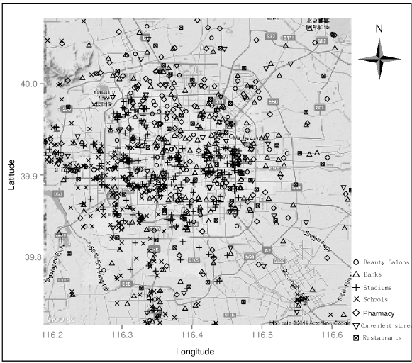
Figure 1: The distribution of 7 facilities in Beijing.

    Through Baidu Map API, we obtain the data set of spatial coordinates of 7 facilities, in the city area and adjacent counties and county-level cities of 37 major cities in China. The 7 facilities are: beauty salons, banks, stadiums, schools, pharmacy, convenient stores and restaurants. The 37 major cities consist of 4 direct-controlled municipalities (Beijing, Shanghai, Chongqing, Tianjin), 30 Provincial capitals and sub-provincial cities and 3 other large cities. The spatial data is the latitude and longitude coordinates of each facility. For example, as shown in Fig. 1, we randomly choose 300 samples for each of the 7 facilities in Beijing and mark these samples in the map. Then we convert the spatial data of the latitude and longitude coordinates into the the plane coordinate data denoted by meter, so as to facilitate the calculation of distance and area selection. Since it is hard to define the exact boundary of a city, we fix the central point $(\textnormal{lng}_{0},\textnormal{lat}_{0})$ of a city, then calculate the relative distance of each sample to the central point in the plane coordinate centered at it. For example, given the latitude and longitude coordinate $(\textnormal{lng}_{i},\textnormal{lat}_{i})$ of a sample, its relative distance to the central point can be defined by: $x_{i}=\textnormal{Distance}((\textnormal{lng}_{i},\textnormal{lat}_{0}),(\textnormal{lng}_{0},\textnormal{lat}_{0}))\times\textnormal{Sign}(\textnormal{lng}_{i},-\textnormal{lng}_{i})$, $y_{i}=\textnormal{Distance}((\textnormal{lng}_{0},\textnormal{lat}_{i}),(\textnormal{lng}_{0},\textnormal{lat}_{0}))$ $\times\textnormal{Sign}(\textnormal{lat}_{i},-\textnormal{lat}_{i})$. Here, $Sing(x)=1$ if $x>0$, 0 if $x=0$, and $-1$ if $x<0$. The relative distance is equal to the length of arc connecting two points on a spherical coordinate. The radius of the earth is given by $R=6371004$ meters .

3 Research Methods

For each city, we choose a $40km\times 40km$ study area centered at the city central point. This area is then divided into 16 $10km\times 10km$ non-overlapping sub-areas, each of which is further divided into 25 $2km\times 2km$ small quadrats. We denote the number of a facility in quadrat $i$ of sub-area $j$ with $X_{ji}$, where $i=1,2,...,25$ and $j=1,2,...16$. For each of the 16 sub-areas, we calculate the mean and variance of the number of a facility, thus getting 16 pairs of mean and variance denoted by $(m_{j},S_{j}^{2})$, where $m_{j}=E[X_{j}]$ and $S_{j}^{2}=Var(X_{j})$ ($j=1,2,...16$). In order to get a good estimation of mean and variance in each sub-area $j$, $X_{i,j}$ should be bigger than 0 for a sufficient number of quadrats. However, because of the irregularity of the city area, a few of the sub-areas could be corresponding with the depopulated zones, such as sea and mountainous areas. Hence, for some cities, the numbers of the pairs of means and variances are less than 16. Nonetheless, this would not affect the robustness of the analytical results in this paper.

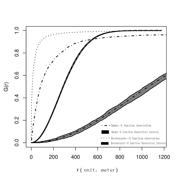
Figure 2: G function analysis

3.1 Descriptive Statistical Analysis of the spatial distribution of the Facilities

    First of all, we study the statistical characteristics of the distribution of $X_{ji}$. The main objective is to find out whether or not they are from the Poisson distribution, based on $\chi^{2}$ test, $G$ function analysis, and Monte Carlo simulation.

3.2 Taylor’s Power Law

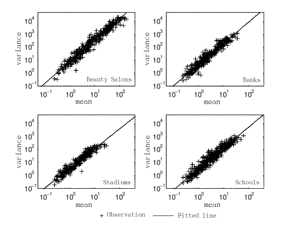
Figure 3: Aggregated scatterplots for Beauty Salons, Banks, Stadiums and Schools.

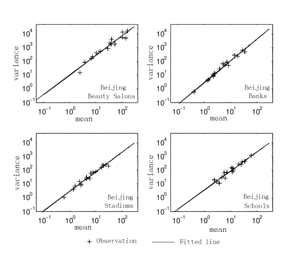
Figure 4: Scatterplots for Beauty Salons, Banks, Stadiums and Schools in Beijing.

    In order to study the statistical characteristics of the spatial distribution of the facilities. we will focus on studying the exponent $b$ in Taylor’s power function $S^{2}=am^{b}$. In some of the cities, the numbers of certain facilities are not large enough, which may greatly increase the size of error in the estimation of the means and variances. To solve this problem, for the study of a facility, we only use the date from the cities which rank in the top 30 in term of the number of this facility. Note that every pair of means and variances is from an area with the same size to the other ones’. Hence, the potential relation between the means and variances only reflects the feature of the events in the areas with a fixed size, not a scaling rule where the number of events is measured in a series of expanding areas discussed by Wu (2014).

Through examining whether or not there is linear correlation between the natural Logarithm values of the means and variances, i.e. $\log S^{2}=loga+b\log m$, we can judge whether or not Taylor’s power law is applicable in the distribution of the urban facilities.

Table 1: Aggregated parameter fitting results of Taylor’s law.

Urban Facilities	Beauty Salons	Banks	Stadium	Schools	Pharmacy	Convenient Stores	Restaurants
$b$	1.66	1.63	1.52	1.61	1.50	1.64	1.74
$\log a$	2.03	1.52	1.30	1.16	1.55	1.55	1.82

4 Analytical Results

4.1 Aggregation Test

By dividing the $40km\times 40km$ study area of each city into $2km\times 2km$ quadrats, and counting the number of events in each quadrat, we can first apply statistic test to see whether urban facilities are aggregated or not. First, the $\chi^{2}$ test is applied against the null hypothesis that urban facilities follow Poisson distribution. For all the 7 facilities in each of the 37 cities, based on the $\chi^{2}$ score of $T_{cc}$, we find that $T_{cc}$ is significantly larger than the result from the Poisson distribution. Under the significance level $\alpha<0.001$, we can reject the null hypothesis of Poisson distribution. For the detailed results for five cities: Beijing, Shanghai, Guangzhou, Chengdu and Wuhan, please refer to Table A1 in Appendix 1.

We also carry out G function analysis on the spatial distribution of the facilities in each city. $G$ function is defined as the distribution function of the nearest neighbour distance. For example, the dashed and the dotted line in Fig. 2 represent the G function of the restaurants and that of the banks in Beijing respectively. In order to illustrate that the two considered facilities are aggregated, we plot the empirical G functions together with the theoretic G functions if the facilties are Poisson distributed. Suppose that the restaurants and the banks in Beijing follow the Poisson distribution, whose parameters are estimated from the real data by assuming that it is Poisson distributed. Then these estimated parameters can be used to generate 99 groups of sample data for each facility by Monte Carlo simulation. After calculating the G functions of those sample data, we can get the envelope of those G functions by taking the maximum and minimum at each distance $r$. The envelope of G functions approximate the 99% confidence interval. The theoretical envelopes of restaurants and banks in Beijing are plotted as the shaded area in Fig.2. We find that the empirical G functions always lie above the confidence interval of the random spatial distribution from the Monte Carlo simulation. Both dotted line and dashed line in Fig. 2 which represents the restaurants and banks in Beijing rises sharply within the range of 200 meters, which implies that the percentage of other facilities locating close to a given facility is far bigger than that can be predicted by random spatial distribution. The restaurants and banks are aggregated in space.

Figure 5: The values of exponent b for 21 cities.

4.2 Taylor’s Power Law

In this subsection, we will examine the aggregated distribution characteristic of each facility in all 30 cities chosen for this facility. Figure 3 shows the scatterplot of the means and variances for each of the four types of facilities, beauty salons, stadiums, schools and banks, in 30 cities corresponding with each of them. The results of the other three facilities (pharmacy, convenient stores, and restaurants) are similar. As we can see from this figure, all the means and variances of each facility are distributed along a straight line in the log-log plot coordinates, which means they could be described by the power function, i.e., they satisfy Taylor’s power Law.

Based on the linear regression of the means on the variances, we can estimate the values of the parameters in Taylor’s power function for each facility. For example, the regression result for schools is: $\log S^{2}=1.16+1.61\log m$, thus the corresponding intercept and slope are given by $\log a=1.16$ and $b=1.61$ respectively. $b>1$ indicates that schools follows the aggregated distribution, which is consistent with statistical test results in the above subsection. Since there is no characteristic scale for the power function, this implies the aggregation degree of schools is similar at various levels of mean concentration. Moreover, for the t-test on the intercepts and slops, the significance levels are all well below 0.001. The null hypothesis that either intercept or slope is zero can be rejected. Besides the four types of facilities in Figure 3, the analytical results of the rest three kinds show that their spatial distributions are all consistent with Taylor’s law. It is worthy noting that values of the intercepts concentrate in the interval $[1.50,2]$.

In the above, we have examined the aggregated distribution of the facilities in 30 cities. Now we examine the distribution of the facilities in a single city. Taking Beijing as an example, we draw the scatterplots of the means and variances for beauty salons, stadiums, schools and banks in Figure 4. As we can see from Figure 4, for each facility, 16 pairs of the means and variances are distributed along a straight line in log-log plot, which clearly indicates that it satisfies Taylor’s law.

Based on the linear regression for each facility in a city, the exponent $b$ falls between 1.0 and 2 (see Table 4), which means that within each city, all the facilities follow aggregation distribution. Once again, the results are consistent with the conclusion from aggregation test.

The graphs in Fig. 3 are derived by the stacking of log-log scatters for all cities. The means and variances are scattered within a band along a straight line, which reflects the fluctuation in the values of exponent $b$ in different cities. The main reasons leading to the fluctuation may lie in the following two aspects. On one hand, the cities are different from each other in terms of their environmental and socioeconomic conditions, which may result in the differences in the slops of the power functions. On the other hand, when the number of a facility is not larger enough, the division of a city into 16 sub-areas may lead to considerable estimation errors of means and variances.

The 7 groups of 30 cities chosen for each facility are different from each other, and there are only 21 cities which are present in all these 7 groups. In order to give a clear picture of the estimation values of exponent $b$ for each facility, we put together the values of exponent $b$ for each facility in those 21 common cities as in Figure 5. As we can see from Figure 5, almost all the values fall between 1 and 2, and concentrate around 1.6. There are some values outside the interval $\left[1,2\right]$, this may result from the the estimation error due to insufficient sample quantity. Despite the differences between the exponent values, the distribution of every facility still complies with Taylor’s law. Based on the existing study of Taylor’s law in ecology, it is reasonable to infer that there are a particular or a few mechanisms underlying the applicability of Taylor’s law in the distribution of urban facilities.

5 Decomposing the Factors Affecting the Number of A Facility

Table 2: The City-Specific Factor in 21 Cities

City	Beijing	Changsha	Chengdu	Dalian	Guangzhou	Haerbin	Hangzhou
$C_{i}$	0.26	0.13	0.18	0.11	0.21	0.11	0.15
City	Hefei	Jinan	Kunming	Nanjing	Qingdao	Shanghai	Shenzhen
$C_{i}$	0.14	0.14	0.18	0.13	0.12	0.23	0.19
City	Shenyang	Shijiazhuang	Taiyuan	Wuhan	Xi’an	Zhengzhou	Chongqing
$C_{i}$	0.15	0.12	0.14	0.16	0.13	0.15	0.13

Table 3: The Facility-Specific Factor for 7 Facilities

Urban Facilities	Beauty Salons	Banks	Stadium	Schools	Pharmacy	Convenient Stores	Restaurants
$f_{j}$	0.44	0.44	0.49	0.48	0.53	0.47	0.43

As we have mentioned in subsection 4.2, the differences in socioeconomic conditions of the cities and the distinct features of various facilities may result in the differences between the values of exponent $b$ in the power functions. In order to explain the fluctuation in the values of $b$ for various facilities and in different cities, we can decompose the factor affecting the number of a facility in the quadrats of a city into two main factors: city-specific factor and facility-specific factor. Through the ordinary least square regression, this decomposition may remove a proportion of estimation error due to insufficient sample quantity, so that we can illustrate the relative contributions of CSF and FSF to the number of a facility in the quadrats of a city.

Assume: a) the number of a facility in a quadrat of a city is jointly determined by the CSF and FSF, which are assumed to be independent from each other; b) these two factors satisfy the following equation for decomposition: $X_{ij}=Y_{i}+Z_{j}$, where: a) $X_{ij}$ stands for the quantity of the facility $j$ ($j=1,2,...,7$), in a quadrat of city $i$ ($i=1,2,...,21$); b) $Y_{i}$ represents the CSF; and c) $Z_{j}$ represents the FSF. It is clear that the mean value of $X_{ij}$ could be expressed as:

$$m_{ij}=\textnormal{E}(X_{ij})=\textnormal{E}(Y_{i})+\textnormal{E}(Z_{j})=m_{Y_{i}}+m_{Z_{j}},$$ (1)

where $m_{Y_{i}}=\textnormal{E}(Y_{i})$ and $m_{Z_{j}}=\textnormal{E}(Z_{j})$, which represent the average contribution value of the CSF and that of the FSF respectively. We further assume that there is a power function relation with exponent $c_{i}$ between the variance $S^{2}$ and the average contribution value of the CSF, while the power function for FSF is with exponent $f_{i}$. This assumption can be represented by the following two equations:

$$m_{Y_{i}}=(S_{ij}^{2})^{c_{i}}/\tilde{a},$$ (2)

$$m_{Z_{i}}=(S_{ij}^{2})^{f_{i}}/\tilde{a}$$ (3)

Here, it is assumed that there is a common factor $\tilde{a}$ in the above two power functions. It should be noted that when $S_{ij}^{2}$(or $m_{ij}$) is sufficiently large, these two power functions will play a dominant role, making this assumption relatively trivial. By combining equations (2) and (3), we have:

$$\frac{m_{Y_{i}}}{m_{Z_{i}}}=S_{ij}^{2(c_{i}-f_{i})},$$ (4)

which means that the relative average contribution, between the CSF and the FSF, is determined by the difference between the exponents $c_{i}$ and $f_{i}$. Particularly, when $S_{ij}^{2}\gg 1$ (or $m_{ij}\gg 1$) is sufficiently large, the factor corresponding to the relative larger exponent between $c_{i}$ and $f_{i}$, will play an absolutely dominant role in the average contribution to the number of a facility in an area. For instance, when $f_{i}>c_{i}$, the FSF plays an absolutely dominant role.Based on the Taylor’s power function $S^{2}=am^{b},$ we can derive:

$$m_{ij}=(S_{ij}^{2})^{\frac{1}{b_{ij}}}/a^{\frac{1}{b_{ij}}}$$ (5)

Hence, based on Eqs. (1), (2), (3) and (5), we can infer:

$$(S^{2})^{\frac{1}{b_{ij}}}=(S_{ij}^{2})^{c_{i}+f_{i}},$$ (6)

thus,

$$\frac{1}{b_{ij}}=c_{i}+f_{i}$$ (7)

Considering the errors in the data, we can rewrite Eq. (7) as:

$$\frac{1}{b_{ij}}=c_{i}+f_{i}+\varepsilon_{ij}.$$ (8)

Based on Eq. (8), we can define the objective function:

$$J=\sum_{i=1}^{n}\sum_{j=1}^{m}\left(\frac{1}{b_{ij}}-(c_{i}+f_{i})\right)^{2},$$ (9)

where $n$ and $m$ represent the number of cities and that of a facility respectively. Through minimizing the above objective function, we can derive the value of $c_{i}$ and that of $f_{i}$. We find that $E[|\frac{1}{b_{ij}}-(c_{i}+f_{i})|/\frac{1}{b_{ij}}]=2.7\%$, which means that $c_{i}$ and $f_{i}$ jointly contribute $97.3\%$ to the value of $\frac{1}{b_{ij}}$. The vast majority of the values of $c_{i}$ fall between 0.1 and 0.26, contributing around 25% to the value of $\frac{1}{b_{ij}}$; while the values of $f_{i}$ are rather concentrated in a small interval $[0.43,0.53]$, contributing about $75\%$ to the value of $\frac{1}{b_{ij}}$. Hence, it is obvious it is the FSF that plays a dominant role in determining the number of a facility in an area within a city. Based on the above analysis, we can infer that when the number of a facility in an area is relative large, it is largely the FSF that leads to the agglomeration of the facility; while the role of city-specific factor is minor.

In order to better understand the above analytical results, let’s look at the case of beauty salons in Beijing. The relevant values for this case is given by: $c=0.26$, $f=0.44$, $\log(a)=2.23$ and $b=1.42$. When the variance $S^{2}=5000$, the mean value of this facility in a quadrat in Beijing is: $m=(S^{2})^{\frac{1}{b}}/a^{\frac{1}{b}}$. The average contribution of the CSF for Beijing is: $m_{Y}=(S^{2})^{c}/a^{\frac{1}{2b}}$, and the average contribution of the FSF is: $m_{Z}=(S^{2})^{f}/a^{\frac{1}{2b}}$. Based on these values, it is clear that the FSF plays a dominant role in the mean value of beauty salons in a quadrat in Beijing. In the following two tables, we list the values of the contribution factors for all the 7 facilities in 21 cities.

As we can see from Table 2, the values of the CSF vary significantly among different cities. These values directly determine the mean value for all facilities in a quadrat within a city, hence they can be seen as the indicators of the overall density of all the facilities in their corresponding cities. The CSF for Beijing is 0.26, which shows the highest density of the facilities among all the cities. It is followed by Shanghai (0.23), Guangzhou (0.21). Dalian and Haerbin have the same lowest value of the CSF at 0.11.

For the values of the FSF, we need to understand from another perspective. Because $\frac{1}{b_{ij}}=c_{i}+f_{j}$, for given a value of $c_{i}$ in a city, the smaller the value of $f_{j}$, the larger the values of $b_{ij}$ and therefore larger $S_{ij}^{2}$ for a given mean $m_{ij}$ in the corresponding city. Larger variances imply greater differences between the numbers of facility $j$ in different quadrats. At some place, the number is small, but at another place, the number can be very large which means that the facility tend to aggregate in space. On the contrary, when $f_{j}$ becomes larger, given the same value of mean, the variance falls, thus the distribution tends to behave more like the Poisson distributio, which implies a weaker aggregation. In our decomposition, the value of the FSF for restaurants is 0.43, which is the smallest, and that for pharmacy is 0.53, which is the largest. This shows restaurants have the highest degree of aggregation; while pharmacy has the lowest degree of aggregation. Restaurants with different styles can coexist at one place, however, due to its interchangeability, pharmacy tends to distribute away from each other.

6 Discussion

Industries are often geographically concentrated in particular cities or metropolitan areas, and there are many theories explaining why the concentration may occur (Marshall (2006); Krugman (1990); Ellison and Glaeser (1999). According to Marshall (2006), industries agglomerate mainly because of the following factors: (i) benefiting from mass-production (internal economies or scale economies), ii) saving transport costs by proximity to input suppliers or final consumers, iii) allowing for labor market pooling, iv) facilitating knowledge spillovers by reducing communication cost, and v) capitalizing from the existence of modern infrastructures. Ellison and Glaeser (1999) assess the importance of natural advantage to geographic concentration, and find that one-quarter of industrial concentration can be explained by observable sources of natural advantage. Krugman (1990) develops a model of labor market pooling, illustrating how labor market pooling leads to industrial agglomeration. Audretsch (1998) states that ‘knowledge is generated and transmitted more efficiently via local proximity, economic activity based on new knowledge has a high propensity to cluster within a geographic region’.

The analytical results in this paper are in line with the findings in the literature mentioned in the above paragraph. Beijing, Shanghai and Guangzhou are generally acknowledged as the three most urbanized cities in China, and our analytical results show that these three cities have the highest level of concentration of urban facilities. Glaeser and Kohlhase (2004) show evidence that services tend to be located in dense areas because they are more dependent on proximity to costumers than manufacturing industries. Kolko (2007) states that services are less agglomerated but more urbanized than manufacturing. Moreover, there is a strong tendency of service industries to locate near their suppliers and customers, because the costs of delivering services are much higher than the costs of delivering goods. City streets enable service providers to readily link with large numbers of their diverse customers, hence they are a good setting for services. Waldfogel (2008) reveals that there is a strong pattern of retail establishment sectors, such as restaurants and media, to locate near demographic groups that regularly buy from that sector.

6.1 Animal Grouping Behavior and Facility Aggregating Pattern

As we have shown in the above analyses, the distribution of urban facilities resembles that of the organisms in ecosystems. Organisms feed on various resources, while facilities ‘feed on’ consumer demand. Organisms are prone to form groups, but the size of group varies between different species. For example, zebras and wildebeest form large herds, while the lions usually live in small groups. Urban facilities tend to agglomerate in an area, while as we can see from Table 3, the degree of agglomeration varies between different facilities. For instance, the value of the FSF for restaurants is 0.43, which is the smallest, and that for pharmacies is 0.53, which is the largest. This shows restaurants have the highest degree of agglomeration; while pharmacies have the lowest degree of agglomeration (or highest degree of dispersion). The same facilities in an area may help each other survive, but at the same time, they compete with each other in various aspects(such as consumer demand and raw materials), which resembles the relationship between the organisms of a specie in an area.

Considering the similarities between organisms and urban facilities, we may get a useful guideline in the study of the reasons driving the agglomeration of facilities, through looking at the factors contributing to the concentration of organisms.

i) Some organisms agglomerate in an area, because their food is clumped. As long as there is no pending threat, animals will stop moving and searching when they reach an area with abundant food. Animals of the same species survive on the same food, thus an area abundant with such food will attract them to move from other areas. As a result, they start to concentrate in this area. Examples include various herbivores, such as zebras, chinkaras and fallow deers.

Across services, Kolko (2007) finds a positive relationship between urbanization and concentration, and the services that are most likely to benefit from geographic connections to diverse urban populations, are also most likely to concentrate. Many urban facilities, such as restaurants, beauty salons, stadiums and schools, deliver face-to-face services or serve as venues of meeting people, while the costs of moving people across space is much higher than that of delivering products. Hence, urban facilities would concentrate in those areas where their customers are concentrated. For instance, the restaurants tend to agglomerate in those business areas with large numbers of visitors, i.e. their customers are ‘clumped’.

ii) The larger a group, the less likely it is an individual will be eaten, because your risk is diluted by those around you. Grouping has been widely accepted as a mechanism for protection from predation. Moreover, Mooring and Hart (1992) point out that grouping applies as much to protection of animals from flying parasites as protection from predators, as long as the encounter-dilution effect works. They state: ‘the encounter-dilution effect provides protection when the probability of detection of a group does not increase in proportion to an increase in group size (the encounter effect), provided that the parasites do not offset the encounter effect by attacking more members of the group (the dilution effect)’.

If a number of certain facilities have been surviving in an area, their success signals to the potential enters that this area is a desirable location for their business, thus it is less likely that their business would fail. Such a signaling effect may attract more and more same facilities into this area or adjacent areas, thus urban facilities agglomerate. Moreover, when the number of adverse incidents, such as robbery and extortion, does not increase in proportion to an increase in group size, an individual facility could become less likely to suffer from those adverse incidents. This ‘dilution effect’ could be another reason driving the agglomeration of urban facilities.

iii) By living in groups, many prey species become faster in detecting approaching predators and stronger in defending against them. Goshawks are less successful in attacks on pigeons in large flocks mainly because the pigeons are much more alerted to a pending attack sufficiently early to fly away. Fish swim together in schools to warn each other of approaching danger. Moreover, when many group-living animals are confronted with predators, they will resort to mobbing behavior to defense themselves.

Urban facilities agglomerating in an area are facing similar market conditions and potential negative shocks, such as unexpected changes in consumer preference. By observing what is happening to their peers in the same industry and communicating with them, the owners of the facilities may be able to detect the changes in the market earlier. Such a knowledge spillover effect could enable them to adapt to the changes in time, so as to improve business performance or reduce loss. Moreover, when there exist certain group defense mechanisms between the same facilities in an area, each individual facility will become less vulnerable to potential threats. For example, the restaurant owners may cooperate with each other to exert greater pressure on the supplies who are planning to increase the prices of raw materials.

iv) For many organisms, the success of finding food is directly related to the size of group. The desert locusts usually move in swarms of immense size, which enable them to spot forage efficiently. Naked mole-rats live in groups of up to 300, and they establish co-ordinated digging teams in their attempts to find hidden food below ground. Couzin et al. (2005) finds that the larger the group, the smaller the proportion of informed individuals needed to guide the group on the move. Moreover, only a very small proportion of informed individuals is required to achieve great accuracy of direction.

For many urban facilities, the success of attracting more customers is directly related to the size of group.When the number of certain facility grows in an area, this may work as a ‘free advertisement’ to the population in this area and those adjacent areas. Large numbers of same facilities in an area usually imply that the consumers are entitled to more differentiated services and possible lower prices, especially for those monopolistic competition industries (such as restaurants and beauty salons). This may attract more customers from this area and other areas. Moreover, As we have mentioned in the above, many urban facilities are served as venues for meeting people. When people are discussing about where to meet, it is more likely that they would agree on the location where the facilities concentrate, instead of those areas with only a few such facilities. Examples include restaurants and fashion shops.

Animals can benefit from the positive side of grouping, while at the same time, they have to live with the negative side. Animals may face some threats resulting from grouping. The dawn cacophony at a sociable weaver nest attracts various predators, including cape cobra. Individuals within groups also share adverse attributes such as parasites and diseases. Moreover, it is paradoxically yet naturally that the very group members that assist you to either find or subdue your food, will instantly become your greatest rivals when the time comes to eat the spoils. Naked mole-rats co-ordinated in digging for food below ground, nonetheless once food is found, the veneer of co-operation gives way to conflict immediately.

When the number of restaurants grows in an area within a city, this may attract more customers from other areas; while at the same time, a restaurant will have to compete with more rivals for the customers in this area. Belleflamme et al. (2000) state “when the firms in the same industry are agglomerated, they will have to face the prospects of tough price competition”. This conclusion could also be applied to those facilities in the service industry. Moreover, Belleflamme et al. (2000)argue that the price competition can be relaxed through product differentiation. Generally speaking, the products or services are more differentiated in the restaurants, this could explain why the restaurants are more agglomerated than other types of facilities.

6.2 External Economy vs. External Diseconomy of Agglomeration

Figure 6: External economy vs. external diseconomy.

Figure 7: Equilibrium levels for different facilities.

Figure 8: Equilibrium levels of clustering across areas.

The theory of agglomeration economies proposes that firms enjoy positive externalities from the spatial concentration of economic activities. These benefits can arise from both intra- and inter-industry clustering of economic activities (see Fujita et al. (1999); Fujita and Thisse (2002)). Fujita and Thisse (2002) state: ‘Intuitively the equilibrium spatial configuration of economic activities can be viewed as the outcome of a process involving two opposing types of forces, that is, agglomeration (or centripetal) forces and dispersion (or centrifugal) forces…an interesting model of economic geography must include both centripetal and centrifugal forces. The corresponding spatial equilibrium is then the result of a complicated balance of forces that push and pull consumers and firms until no one can find a better location’.

In the context of economics, we may use external economy and external diseconomy of clustering to describe the opposite impacts of increasing the number of the same type of facilities in an are. In order to study the distribution pattern of urban facilities, and the differences between the distribution patterns of various urban facilities, we need to explore the factors leading to external economy or external diseconomy, and examine the differences between these factors and how they affect the patterns. Facilities such as restaurants and beauty salons are more concentrated than some other facilities such as pharmacies and stadiums, because for the former, external economy dominates external diseconomy over larger numbers of agglomerated facilities, compared with the later.

A potential entrant is determining whether or not to locate his business in an area with n incumbent, where $n\geq 0$. Suppose the external economy will bring extra $f(n)$ units of profit to his business, while the external diseconomy will reduce the profit by $g(n)$ units. Here, let’s assume: i) $f(n)$ is concave function with $f(0)=0$, $f′(0)=\infty$, $f′(n)>0$ and $f′^{\prime}(n)<0$ for all $n>0$; ii) $g(n)$ is a convex function with $g(0)=0$, $g′(0)=0$, $g^{\prime}(n)<0$ and $g′′(n)>0$, for all $n>0$. We may normalize the profit from locating the business in other areas to zero, then the decision rule of the entrant is reduced to comparing the benefit of external economy and the cost of external diseconomy.

In Figure 6, the unique crossing point of $f(n)$ and $g(n)$ is corresponding to the number $n^{*}$. It is clear that when the number of incumbents in an area is $n^{*}$, the potential entrant is indifferent between entering this area or not. When the number of incumbents is smaller than $n^{*}$, the potential entrant will enter. When the number of incumbents is larger than $n^{*}$, the potential entrant will not enter; Hence, given the the above simple setting, the equilibrium level of clustering is $n^{*}$ for the same type facilities in an area.

The degrees of agglomeration vary across different facilities, which means the equilibrium levels of clustering are different between facilities. This results from different extent of external economy and external diseconomy. Suppose there are l types of facilities. In order to reflect such a difference, we can introduce a parameter $\alpha_{i}$, where $\alpha_{i}>0$ and $i=1,2,...l$, to scale up or scale down external economy; and a parameter $\beta_{i}$, where $\beta_{i}>0$, to scale up or scale down external diseconomy. For type $i$ facilities, the external economy and external diseconomy are represented by $\alpha_{i}f(n)$ and $\beta_{i}g(n)$ respectively. There is an unique crossing point of $\alpha_{i}f(n)$ and $\beta_{i}g(n)$ corresponding to $n_{i}^{*}$, which is the equilibrium level of clustering for type $i$ facilities. By comparing the $n_{i}^{*}$ for different types, we can find out which type has higher degree of agglomeration. For example, if $\beta_{i}=\beta_{j}$, while $\alpha_{i}>\alpha_{j}$, where $i\neq j$, then it is easy to show $n_{i}^{*}>n_{j}^{*}$ (see Figure 8).

As we have shown, the concentration level of a facility varies across cities and different areas within a city. Certain specific features of an area, such as population density and location, may have significant impact on the the concentration level of a facility. Suppose there are h areas, we may introduce parameter $\theta_{ij}$ and $\eta_{ij}$ , where $j=1,2,...,h$ , to represent the area-specific impact on external economy and external diseconomy for facility $i$ , where $i=1,2,...l$ . Here, $\theta_{ij}\in[\underline{\theta_{i}},\overline{\theta_{i}}]$ and $\eta_{ij}\in[\underline{\eta_{i}},\overline{\eta_{i}}]$ , where $\overline{\theta_{i}}>\underline{\theta_{i}}>0$ and $\overline{\eta_{i}}>\underline{\eta_{i}}>0$. Then $\theta_{ij}\alpha_{i}f(n)$ and $\eta_{ij}\beta_{i}g(n)$ stand for the external economy and external diseconomy for facility $i$ in area $j$ respectively, where $i=1,2,...l$ and $j=1,2,...,h$ . It is clear that for facility $i$ in area $j$ , the lowest equilibrium level of clustering $n_{\textnormal{min}}$ is jointly determined by $\underline{\theta_{i}}\alpha_{i}f(n)$ and $\overline{\eta_{i}}\beta_{i}g(n)$ , while the highest level $n_{max}$ is jointly determined by $\overline{\theta_{i}}\alpha_{i}f(n)$ and $\underline{\eta_{i}}\beta_{i}g(n)$ . This can be shown in figure 8.

7 Conclusion

Based on the data set of spatial coordinates of 7 facilities in 37 major cities in China, we explore the micro-structure of these cities and study the characteristics of the distribution of urban facilities. We find that there is a power law function relationship $S^{2}=am^{b}$ between the variance $S^{2}$ and mean number $m$ of facilities in the quadrats, and almost all the values of exponent $b$ falling between 1 and 2. This shows that the distribution of urban facilities complies with Taylor’s law. The same facilities in a city may help each other survive, while at the same time, they compete for various resources, which resembles the relationship between the organisms of a specie in an area.

Furthermore, in order to study the key factors contributing to the difference between the values of exponent $b$ and explore the mechanism underlying the distribution of urban facilities, we decomposing the inverse of exponent $b$ into two different factors contributing to the numbers of facilities in a city respectively: the CSF and the FSF. we find that the values of the CSF vary significantly between different cities, and different facilities have different degree of agglomeration. It is interesting to note that Beijing, Shanghai and Guangzhou, the three largest and most developed cities in mainland China, show the highest density of the facilities among all the cities. Moreover, restaurants have the highest degree of agglomeration; while pharmacies have the lowest degree of agglomeration. These findings are consistent with our intuitive understandings of these cities and urban facilities.

Spatial Statistics has been becoming more and more important in urban and regional studies, which greatly contributes to the development of theories and knowledge in this field. Through studying the characteristic of the spatial distribution of urban facilities, we can find out whether or not there is an agglomeration property of a facility and how strong it is. Bettencourt and West (2010) state: ‘…cities are remarkably robust: success, once achieved, is sustained for several decades or longer, thereby setting a city on a long run of creativity and prosperity’. While the distribution of urban facilities may play a critical role in setting a city on a long run of creativity and prosperity.

It is important for us to carry out further studies on the distribution of urban facilities, and the potential directions could lie in the following three aspects. Firstly, through combining spatial statistics, economic theories and other relevant fields, we could further explore the rationals and mechanisms underlying the distribution of urban facilities, and examine its impact on socioeconomic development in a city and the adjacent regions. Secondly, when we have sufficient panel data, we could examine the evolution of the distribution of urban facilities over both the time and space, and explore the relationship between the evolution process and the changes in socioeconomic development indicators, such as income per capita, population density and health indicator, etc. Lastly, we could explore relevant theoretical frameworks that could help improve the distribution of urban facilities, thus facilitating sustainable development of cities.

Appendix

Table 4: The Analitical Results of 7 urban facilities in Five Representative Cities

City	Ss.	Convenient Stores	Restaurants	Beauty Salons	Stadiums	Schools	Pharmacy	Banks
Beijing	$n$	9142	56844	25405	3768	6660	3719	3521
	$T_{cc}$	11312.2	122323.9	82491.4	6841.6	12257.4	3968.5	9261.9
	$p$	(0.000)	(0.000)	(0.000)	(0.000)	(0.000)	(0.000)	(0.000)
	$b$	1.25	1.39	1.42	1.42	1.37	1.25	1.57
Shanghai	$n$	14038	59065	23194	3079	5519	2939	2923
	$T_{cc}$	26667.0	170349.1	77446.1	6935.5	10858.1	3534.1	10940.6
	$p$	(0.000)	(0.000)	(0.000)	(0.000)	(0.000)	(0.000)	(0.000)
	$b$	1.64	1.75	1.78	1.51	1.61	1.50	1.58
Guangzhou	$n$	7575	25824	11626	1411	3784	4408	2063
	$T_{cc}$	22213.6	71082.8	52938.8	4567.7	8491.2	7871.3	9251.2
	$p$	(0.000)	(0.000)	(0.000)	(0.000)	(0.000)	(0.000)	(0.000)
	$b$	1.55	1.38	1.48	1.43	2.06	1.80	1.59
Chengdu	$n$	9540	32121	12470	869	3469	4711	1606
	$T_{cc}$	30919.1	158292.7	67452.3	4266.7	8926.94	10328.6	7816.2
	$p$	(0.000)	(0.000)	(0.000)	(0.000)	(0.000)	(0.000)	(0.000)
	$b$	1.54	1.55	1.58	1.72	1.72	1.20	1.63
Wuhan	$n$	4443	18406	7684	1027	3168	3103	1397
	$T_{cc}$	20633.4	99795.5	44907.7	4176.0	10303.7	11772.3	6427.0
	$p$	(0.000)	(0.000)	(0.000)	(0.000)	(0.000)	(0.000)	(0.000)
	$b$	1.61	1.78	1.68	1.65	1.57	1.63	1.70

Note: a) Ss. stands for statistics; b)$n$ is the total number of facilities; c)$T_{cc}$ is the statistical score of $\chi^{2}$; d)$p$ is the p-value of $\chi^{2}$ test; e) b is the exponent in Taylor’s power function.

References

- Andersen and May (1988) Andersen, R. M., May, R. M., 1988. Epidemiological parameters of hi v transmission. Nature 333 (6173), 514–519.
- Anderson et al. (1982) Anderson, R., Gordon, D., Crawley, M., Hassell, M., 1982. Variability in the abundance of animal and plant species. Nature, 245–248.
- Audretsch (1998) Audretsch, B., 1998. Agglomeration and the location of innovative activity. Oxford review of economic policy 14 (2), 18–29.
- Belleflamme et al. (2000) Belleflamme, P., Picard, P., Thisse, J.-F., 2000. An economic theory of regional clusters. Journal of Urban Economics 48 (1), 158–184.
- Bettencourt and West (2010) Bettencourt, L., West, G., 2010. A unified theory of urban living. Nature 467 (7318), 912–913.
- Bettencourt et al. (2007) Bettencourt, L. M., Lobo, J., Helbing, D., Kühnert, C., West, G. B., 2007. Growth, innovation, scaling, and the pace of life in cities. Proceedings of the National Academy of Sciences 104 (17), 7301–7306.
- Botkin and Beveridge (1997) Botkin, D. B., Beveridge, C. E., 1997. Cities as environments. Urban Ecosystems 1 (1), 3–19.
- Couzin et al. (2005) Couzin, I. D., Krause, J., Franks, N. R., Levin, S. A., 2005. Effective leadership and decision-making in animal groups on the move. Nature 433 (7025), 513–516.
- Ellison and Glaeser (1999) Ellison, G., Glaeser, E. L., 1999. The geographic concentration of industry: does natural advantage explain agglomeration? American Economic Review, 311–316.
- Fujita et al. (1999) Fujita, M., Krugman, P., Venables, A. J., 1999. The spatial economy: Cities, regions, and international trade.
- Fujita and Thisse (2002) Fujita, M., Thisse, J.-F., 2002. Economics of agglomeration: Cities. Industrial Location, and Regional Growth, Cambridge.
- Girardet (1996) Girardet, H., 1996. The Gaia Atlas of Cities: new directions for sustainable urban living. UN-HABITAT.
- Glaeser and Kohlhase (2004) Glaeser, E. L., Kohlhase, J. E., 2004. Cities, regions and the decline of transport costs*. Papers in Regional Science 83 (1), 197–228.
- Hall (1998) Hall, P. G., 1998. Cities in civilization. Pantheon Books New York.
- Kendal (2004) Kendal, W. S., 2004. A scale invariant clustering of genes on human chromosome 7. BMC evolutionary biology 4 (1), 3.
- Kolko (2007) Kolko, J., 2007. Agglomeration and co-agglomeration of services industries.
- Krugman (1990) Krugman, P., 1990. Increasing returns and economic geography. Tech. rep., National Bureau of Economic Research.
- Linnerud et al. (2013) Linnerud, M., Sæther, B.-E., Grøtan, V., Engen, S., Noble, D. G., Freckleton, R. P., 2013. Interspecific differences in stochastic population dynamics explains variation in taylor’s temporal power law. Oikos 122 (8), 1207–1216.
- Marshall (2006) Marshall, A., 2006. Industry and trade. Vol. 2. Cosimo, Inc.
- Miller (1978) Miller, J. G., 1978. Living systems.
- Mooring and Hart (1992) Mooring, M. S., Hart, B. L., 1992. Animal grouping for protection from parasites: selfish herd and encounter-dilution effects. Behaviour, 173–193.
- Mumford (1961) Mumford, L., 1961. The city in history. its origins, its transformation, and its prospects.
- Philippe (1999) Philippe, P., 1999. The scale-invariant spatial clustering of leukemia in san francisco. Journal of theoretical biology 199 (4), 371–381.
- Rhodes and Anderson (1996) Rhodes, C. J., Anderson, R. M., 1996. Power laws governing epidemics in isolated populations. Nature 381 (6583), 600–602.
- Taylor (1961) Taylor, L., 1961. Aggregation, variance and the mean. Nature, 732–735.
- Waldfogel (2008) Waldfogel, J., 2008. The median voter and the median consumer: Local private goods and population composition. Journal of Urban Economics 63 (2), 567–582.
- Wu (2014) Wu, L., 2014. Scaling properties of urban facilities. arXiv preprint arXiv:1406.0691.