Chapman-Enskog Analysis of Finite Volume Lattice Boltzmann Schemes

Abstract

In this paper, we provide a systematic analysis of some finite volume lattice Boltzmann schemes in two dimensions. A complete iteration cycle in time evolution of discretized distribution functions is formally divided into collision and propagation (streaming) steps. Considering mass and momentum conserving properties of the collision step, it becomes obvious that changes in the momentum of finite volume cells is just due to the propagation step. Details of the propagation step are discussed for different approximate schemes for the evaluation of fluxes at the boundaries of the finite volume cells. Moreover, a full Chapman-Enskog analysis is conducted allowing to recover the Navier-Stokes equation. As an important result of this analysis, the relation between the lattice Boltzmann relaxation time and the kinematic viscosity of the fluid is derived for each approximate flux evaluation scheme. In particular, it is found that the constant upwind scheme leads to a positive numerical viscosity while the central scheme as well as the linear upwind scheme are free of this artifact.

1 Introduction

In recent years, mesoscopic methods such as stochastic rotation dynamics (SRD) [1, 2], dissipative particle dynamics (DPD) [3, 4] and the lattice Boltzmann method (LBM) [5, 6, 7, 8, 9] appeared as alternatives to conventional computational fluid dynamic (CFD) methods for the simulation of several complex fluid dynamical problems ranging from two-phase flow through porous media [10], particle-fluid suspensions [11] and high Reynolds number flows [12, 13, 14, 15].

The original lattice Boltzmann method, proposed as probability density based (and hence a coarse grained) counterpart of lattice-gas cellular automata [16, 17, 18], attracted much interest to be a practical computational fluid dynamics tool. However, one of the major drawbacks of the original lattice Boltzmann method was its restriction to uniform lattices, leading to problems when dealing with practical CFD applications. In order to overcome this limitation, many efforts were undertaken to enhance LBM’s efficiency when dealing with complex geometries or multi scale problems which require non-uniform or unstructured grids. These extensions of the standard LBM are generally motivated by the conventional CFD methods. Among the most important techniques are local grid refinement [19, 20, 21], interpolation supplemented finite difference method [22, 23] as well as various types of finite volume formulations [24, 25, 26, 27, 28]. These different approaches extent the lattice Boltzmann method to non-uniform and even unstructured grids. Among these methods, finite volume approaches are of a rather simple and flexible form. As the name suggests, in a finite volume approach, the space is divided into a number of subvolumes, each containing a finite (but not necessarily equal) fraction of the total available volume of the computational domain. When applying to a space spanned by lattice nodes (as is the case in the lattice Boltzmann method), the division of the space is done in such a way as to ensure that each subvolume contains (surrounds) one and only one lattice node. The time evolution (update) of the population densities assigned to a given lattice node is then governed by the net mass current into the subvolume containing that node. Obviously, the net mass flux into a subvolume is computed as the surface integral of the mass flux vector projected onto the direction normal to the surface surrounding the node under consideration. Although finite volume formulations are used extensively, there is still lack of analytical analysis of this type of LBM modifications. There are, however, some theoretical arguments, based on the inspection of the dispersion relation associated with the unstructured lattice Boltzmann scheme [26]. More recently, through establishing a link between the lattice Boltzmann scheme and the finite volume method, general relations that define mass and momentum fluxes is proposed and the treatment of the boundary condition is studied [29]. Here we will perform a full Chapman-Enskog analysis of some typical finite volume approaches to introduce a framework for further analytical investigations. In order to keep the presentation and the subsequent analysis as simple as possible, we choose a two dimensional uniform mesh. This allows us to focus on generic features of different finite volume lattice Boltzmann methods. As shown in Fig. 1, each cell is a square, including one standard LBM grid point, placed at its center. Boundaries of the cell are located in the middle of the standard LBM grid points. This paper is organized as follows. Section 2 is a review of the original lattice Boltzmann method. In sections 3 and 4, we present the evolution of the velocity of each cell during a single time step, considering details of different finite volume schemes. Section 5 describes the multiscale analysis of the finite volume schemes introduced in section 4. Section 6 discusses the results and concludes the paper.

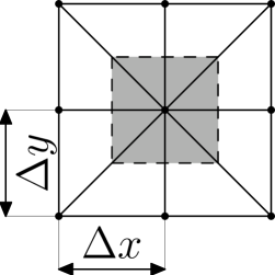
Figure 1: Uniform mesh with $\Delta x=\Delta y$ and the finite volume cell constructed on it (filled with gray). The filled circles are lattice Boltzmann nodes. The time evolution of the population densities at the central node is controlled by the projected (onto the surface normal) sum of all the fluxes entering/leaving the gray region.

2 The Lattice Boltzmann Method

There are excellent monographs [30, 31, 32] and comprehensive review articles [33, 34, 11] on the lattice Boltzmann method and the related lattice-gas cellular automata (LGCA). Historically, the lattice Boltzmann method directly evolved from the lattice-gas cellular automata (LGCA) [16]. Particles represented by Boolean numbers in the LGCA are replaced by single-particle distribution functions. Consequently, the lattice Boltzmann method inherits some properties from the LGCA, including the coupling between the discrete velocity space and the spatial space as well as the conservation of mass and momentum. However, it is important to realize that, despite this historical connection between the LGCA and the LBM, the lattice Boltzmann method can also be derived in a way completely independent of the lattice-gas cellular automata, namely from the kinetic Boltzmann equation in a certain approximation [35]. Similar to the LGCA, dynamics of evolution in the lattice Boltzmann method can formally be divided into two basic steps in each iteration; namely, (i) collision and (ii) propagation. As mentioned above, both mass and momentum are conserved during the collision step. This is a necessary (but not always sufficient) condition in order to recover the correct hydrodynamic behavior in the macroscopic limit. Generally, this property of the collision step is common to all mesoscopic approaches aiming at dealing with hydrodynamic phenomena such as LGCA, LBM, SRD and DPD. In the propagation step of the LGCA or the LBM, on the other hand, the post-collision particles or distribution functions are advected entirely (without any change) along the link connecting two neighboring lattice nodes (free streaming).

Figure 2: Discrete velocities for D2Q9 model

In this paper, we use the two dimensional nine velocity (D2Q9) lattice Boltzmann model (see Fig. 2). Using the so called Bhatnagar-Gross-Krook (BGK) approximation [36], the equation of the evolution of the discretized distribution functions, $F_{i}$ is

$$F_{i}({{\bm{r}}}+{{\bm{c}}}_{i}\Delta t,t+\Delta t)=F_{i}({{\bm{r}}},t)+\omega(F_{i}^{\mathrm{eq}}({{\bm{r}}},t)-F_{i}({{\bm{r}}},t))+\frac{\Delta tc_{i\alpha}}{6c^{2}}K_{\alpha}$$ (1)

where $\Delta t$ is the time step, $\tau$ is the relaxation time and $\omega=\Delta t/\tau$. $F_{i}^{\mathrm{eq}}$ is the equilibrium distribution function, ${\bf K}=(K_{x},K_{y})$ is an applied body force which is assumed to be constant and $\alpha$ indicates different directions of physical coordinate system, $x$ and $y$. In the D2Q9 model used in the present paper, the index $i$ refers to the nine discrete velocities defined by

$${{\bm{c}}}_{i}=\begin{cases}0&i=0\\ (\cos[(i-1)\pi/2],\sin[(i-1)\pi/2])c&i=1,2,3,4,\\ \sqrt{2}(\cos[(i-5)\pi/2+\pi/4],\sin[(i-5)\pi/2+\pi/4])c&i=5,6,7,8.\end{cases}$$ (2)

where $c$ is defined as the ratio of the lattice spacing and the time step, $c=\Delta x/\Delta t$.
Physical properties of the system enter the lattice Boltzmann iteration scheme via the quantity $F_{i}^{\mathrm{eq}}$ equation (1). Obviously, the system is ’pushed’ towards $F_{i}^{\mathrm{eq}}$ with a rate $\Delta t/\tau$. The population density $F_{i}^{\mathrm{eq}}$ is, therefore, referred to as ’equilibrium distribution’. It is noteworthy that the term ’equilibrium’ does not refer to a global thermal equilibrium, where no flow exists. Rather, it describes the local velocity distribution in a portion of fluid moving at a velocity ${{\bm{v}}}({{\bm{r}}})$. Within the present lattice Boltzmann model, one expands $F_{i}^{\mathrm{eq}}$ in powers of the fluid velocity, ${{\bm{v}}}$, up to the second order recalling the second order expansion of the Maxwell velocity distribution. This leads to

$$F_{i}^{\mathrm{eq}}({{\bm{r}}},t)=w_{i}\rho(1+\frac{3({{\bm{c}}}_{i}.{{\bm{v}}})}{c^{2}}+\frac{9({{\bm{c}}}_{i}.{{\bm{v}}})^{2}}{2c^{4}}-\frac{3v^{2}}{2c^{2}})$$ (3)

where the weight factors $w_{i}$ are given by (for a derivation, see e.g. [30])

$$w_{i}=\begin{cases}4/9&i=0\\ 1/9&i=1,2,3,4,\\ 1/36&i=5,6,7,8.\end{cases}$$ (4)

Macroscopic quantities such as density and momentum are obtained locally as the zeroth and the first moments of the population density, $F_{i}$, respectively:

$$\rho=\sum^{8}_{i=0}F_{i}\mbox{~{}~{}~{}~{}~{}~{}~{}~{}~{}~{}~{}~{}~{}~{}~{}~{}~{}and~{}~{}~{}~{}~{}~{}~{}~{}~{}~{}~{}~{}~{}~{}~{}~{}~{}}\rho{{\bm{v}}}=\sum_{i=1}^{8}{{\bm{c}}}_{i}F_{i}.$$ (5)

In order to estimate momentum exchange between cells through their boundaries, the momentum flux tensor is needed. It can be defined as

$$\Pi_{\alpha\beta}=\sum_{i=1}^{8}{{\bm{c}}}_{i\alpha}{{\bm{c}}}_{i\beta}F_{i}.$$ (6)

In the above equation, $\alpha$ and $\beta$ indicate different directions of Cartesian coordinate system, $x$ and $y$. Note that, since ${{\bm{c}}}_{0}=\bm{0}$, the term with $i=0$ has no effect on the fluid velocity as well as the momentum flux tensor. It is of common practice to decompose equation (1) into two parts, the first part is the so called collision step and the second one implements the free propagation (streaming) of the distribution functions between two neighboring lattice nodes directly linked via the velocity vector ${{\bm{c}}}_{i}$. The collision step is considered to occur within a time interval which is infinitesimally small compared to all relevant times in the problem. We therefore consider it as an instantaneous process. The streaming step, on the other hand, happens in the finite time interval $[t,t+\Delta t]$.

$$F^{*}_{i}({{\bm{r}}},t) = F_{i}({{\bm{r}}},t)+\omega(F_{i}^{eq}({{\bm{r}}},t)-F_{i}({{\bm{r}}},t))+\frac{\Delta tc_{i\alpha}}{6c^{2}}K_{\alpha}$$ (7)

$$F_{i}({{\bm{r}}}+{{\bm{c}}}_{i}\Delta t,t+\Delta t) = F^{*}_{i}({{\bm{r}}},t).$$ (8)

It can be easily shown that the requirement of mass and momentum conservation during the collision step is equivalent to the following two conditions on the moments of the distribution function, $F_{i}$, namely

$$\sum_{i=0}^{8}F_{i}({{\bm{r}}},t)=\sum_{i=0}^{8}F_{i}^{\mathrm{eq}}({{\bm{r}}},t)\mbox{~{}~{}~{}~{}~{}~{}~{}~{}~{}~{}~{}~{} and ~{}~{}~{}~{}~{}~{}~{}~{}~{}~{}~{}~{}}\sum_{i=1}^{8}F_{i}({{\bm{r}}},t){{\bm{c}}}_{i}=\sum_{i=1}^{8}F_{i}^{\mathrm{eq}}({{\bm{r}}},t){{\bm{c}}}_{i}.$$ (9)

In the next two sections, we show how the velocity of each cell changes during these two steps in a single iteration cycle.

3 Finite Volume Analysis of the Momentum Change Due to Collision

Although the collision step is modified differently in each finite volume lattice Boltzmann scheme, the mass and momentum conserving properties of the standard lattice Boltzmann method are not violated in any of those schemes. Consequently, the collision step bluedoes not change the momentum of the cells. If an external field is applied, for each cell the velocity of the center of mass will increase by a constant when the external field is constant.

4 Finite Volume Analysis of the Momentum Change Due to Propagation

After the collision step, the system undergoes a propagation step, during which the momentum of cells can change due to the exchange of particles. However, in the standard lattice Boltzmann method, populations, $F_{i}$, are advected entirely (i.e. with no loss or gain) between two neighboring lattice nodes linked along the velocity vector ${{\bm{c}}}_{i}$. In contrast to this, within a finite volume approach, one first determines the total mass flux as well as the momentum flux through the cell’s boundaries by integrating the component of the corresponding current projected onto the direction normal to the cell’s surface. More formally, and considering the case of momentum exchange, one computes the total change in momentum of a cell via

$$\Delta\bm{P}=\Delta t\sum_{i=1}^{8}\int F_{i}{{\bm{c}}}_{i}[{{\bm{c}}}_{i}{\cdot}d{{\bm{S}}}].$$ (10)

Here, the integral is over the whole boundary of a cell. For the simple case of a regular rectangular lattice, each node can be surrounded by a rectangular finite volume cell. In this case, the above integral reduces to

$$(\frac{\Delta P}{\Delta t})_{\alpha} = {\sum_{i=1}^{8}}\int F_{i}c_{i\alpha}[{{\bm{c}}}_{i}\cdot d{{\bm{S}}}]$$ (11)

$$= {\sum_{i=1}^{8}}c_{i\alpha}c_{ix}[F_{i}^{\mathrm{av}}({{\bm{r}}}+\frac{\Delta x}{2}{{\bm{i}}})-F_{i}^{\mathrm{av}}({{\bm{r}}}-\frac{\Delta x}{2}{{\bm{i}}})]\Delta y$$

$$+ {\sum_{i=1}^{8}}c_{i\alpha}c_{iy}[F_{i}^{\mathrm{av}}({{\bm{r}}}+\frac{\Delta y}{2}{{\bm{j}}})-F_{i}^{\mathrm{av}}({{\bm{r}}}-\frac{\Delta y}{2}{{\bm{j}}})]\Delta x.$$

where $F_{i}^{\mathrm{av}}$ is the average of $F_{i}$ over the corresponding edge of the cell. If the edge is horizontal, $F_{i}^{\mathrm{av}}({{\bm{r}}})$ is defined as

$$F_{i}^{\mathrm{av}}({{\bm{r}}})=\frac{1}{\Delta x}\int_{{{\bm{r}}}-\frac{\Delta x}{2}{{\bm{i}}}}^{{{\bm{r}}}+\frac{\Delta x}{2}{{\bm{i}}}}F_{i}(\mathcal{\\ R})d\mathcal{\\ R}$$ (13)

and it is given by

$$F_{i}^{\mathrm{av}}({{\bm{r}}})=\frac{1}{\Delta y}\int_{{{\bm{r}}}-\frac{\Delta y}{2}{{\bm{j}}}}^{{{\bm{r}}}+\frac{\Delta y}{2}{{\bm{j}}}}F_{i}(\mathcal{\\ R})d\mathcal{\\ R}$$ (14)

if the edge is vertical. The first two terms in equation (4) arise from fluxes across the right and left boundaries ($d{{\bm{S}}}=(\Delta y,0)$) whereas the terms proportional to $\Delta x$ represent the contribution of the flux through the top and bottom edges of the cell ($d{{\bm{S}}}=(0,\Delta x)$). In order to simplify the notation, we make use of Einstein summation convention over repeated indices and rewrite equation (4) as

$$(\frac{\Delta P}{\Delta t})_{\alpha} = c_{i\alpha}[F_{i}^{\mathrm{av}}({{\bm{r}}}+\frac{c_{ix}\Delta t}{2}{{\bm{i}}})-F_{i}^{\mathrm{av}}({{\bm{r}}}-\frac{c_{ix}\Delta t}{2}{{\bm{i}}})]c\Delta y$$

$$+ c_{i\alpha}[F_{i}^{\mathrm{av}}({{\bm{r}}}+\frac{c_{iy}\Delta t}{2}{{\bm{j}}})-F_{i}^{\mathrm{av}}({{\bm{r}}}-\frac{c_{iy}\Delta t}{2}{{\bm{j}}})]c\Delta x$$

Thus, for the simple case of a square lattice studied in this work, the computation of the total momentum change within a finite volume cell requires the knowledge of the population density, $F_{i}$, midway between the node surrounded by the cell and the lattice nodes linked to it via a velocity vector ${{\bm{c}}}_{i}$. Since only the values of $F_{i}$ at the lattice nodes are exactly known, some approximation is necessary in order to obtain the required quantities. Therefore, we discuss in the next subsection the details of different methods of evaluating $F_{i}^{\mathrm{av}}$, including the central scheme and constant as well as linear upwind schemes [37]. By conducting a full Chapman-Enskog analysis of these finite volume schemes in section 5, we also study the resulting macroscopic equations and, in particular, the relation between the relaxation time, $\tau$, and the kinematic viscosity, $\nu$, within each approximate method.

4.1 Computation of the Fluxes

As mentioned above, in order to estimate fluxes, $F_{i}^{\mathrm{av}}$ should be evaluated at the cell faces. In the context of finite volume methods, there are many different approaches for flux evaluation [38]. In 1959 Godunov proposed a scheme in which flux evaluation is based on the value of conserved variables which are considered to be piecewise constant over the cells [39]. Later in 1979, van Leer extended the Godunov’s scheme to a higher order total variation diminishing (TVD) method, through use of piecewise linear approximation within each cell and flux limiters [40]. Methods introduced in the finite volume method to solve partial differential equations are implemented in the finite volume lattice Boltzmann method to solve the Boltzmann equation (see e.g. [24, 25, 26, 27, 28]). In this paper, two different upwind schemes introduced by Steibler et al. [37] and one central scheme introduced by Peng et al. [27] are analyzed.

4.1.1 Constant Upwind Scheme

A very simple upwind scheme results from the following approximation

$$F_{i}^{\mathrm{av}}({{\bm{r}}}+\frac{\Delta x}{2}{{\bm{i}}})\simeq F_{i}({{\bm{r}}})\mbox{~{}~{}~{}~{}~{}~{}~{}~{}~{}~{}~{}~{} and ~{}~{}~{}~{}~{}~{}~{}~{}~{}~{}~{}~{}}F_{i}^{\mathrm{av}}({{\bm{r}}}-\frac{\Delta x}{2}{{\bm{i}}})\simeq F_{i}({{\bm{r}}}-\Delta x{{\bm{i}}})$$ (16)

$$F_{i}^{\mathrm{av}}({{\bm{r}}}+\frac{\Delta y}{2}{{\bm{j}}})\simeq F_{i}({{\bm{r}}})\mbox{~{}~{}~{}~{}~{}~{}~{}~{}~{}~{}~{}~{} and ~{}~{}~{}~{}~{}~{}~{}~{}~{}~{}~{}~{}}F_{i}^{\mathrm{av}}({{\bm{r}}}-\frac{\Delta y}{2}{{\bm{j}}})\simeq F_{i}({{\bm{r}}}-\Delta y{{\bm{j}}})$$ (17)

This scheme is the basic Godunov scheme, which simply assumes constant approximations for the value of variables and results in the first order upwind discretization. Inserting equations (16) and (17) into equation (4), $({\Delta P}/{\Delta t})_{\alpha}$ can be estimated as

$$(\frac{\Delta P}{\Delta t})_{\alpha} =c_{i\alpha}[F_{i}({{\bm{r}}})-F_{i}({{\bm{r}}}-c_{ix}\Delta t{{\bm{i}}})+F_{i}({{\bm{r}}})-F_{i}({{\bm{r}}}-c_{iy}\Delta t{{\bm{j}}})]c\Delta x=$$ (18)

$$=c_{i\alpha}[c_{i\beta}\Delta t\partial_{\beta}F_{i}|_{{{\bm{r}}}}-\frac{c_{i\beta}c_{i\gamma}(\Delta t)^{2}}{2}\partial_{\beta}\partial_{\gamma}F_{i}|_{{{\bm{r}}}}+O((\Delta x)^{3})]c\Delta x$$ (19)

It is worth mentioning that, in contrast to central and linear upwind schemes (see equations (27) and (37) ), terms of the second order do not vanish here. As will be shown in section 5 and appendix A, this gives rise to a finite numerical viscosity within the constant upwind approach, an artifact absent both in the central and linear upwind schemes.

4.1.2 Central Scheme

Average value of $F_{i}$ over each face of the cell can be determined by averaging between distribution functions at the both ends of the corresponding face but end points of the cells are not coinciding with the lattice nodes so the values of $F_{i}$ are not known and should be approximated. Each end point has four neighboring lattice nodes and values of $F_{i}$s at these point can be used to interpolate the value of distribution functions at the corresponding end point.

This method is equivalent to the extension of Godunov’s method to use piecewise linear approximation of each cell. Although this method results in second order accuracy in space, it introduces unphysical oscillations in problems with shocks or discontinuities. These spurious oscillations are well-known for higher order schemes (e.g. the Lax-Wendroff scheme [41] and Beam-Warming scheme [42]). These numerical oscillations are due to the non-monotonicity of the higher order schemes[43]. In order to deal with this problem, the concept of flux limiters is introduced into the context of CFD. A systematic analysis and derivation of a class of flux limiters for high resolution TVD second order schemes is done in [44]. Normally, the need for flux limiters arise when there are discontinuities in the problem and in this paper for simplicity we focus on problems with smooth solutions. For such a smooth problem, it can be easily shown that

$$F_{i}^{\mathrm{av}}(r\pm\frac{c_{ix}\Delta t}{2}{{\bm{i}}})\simeq\frac{F_{i}(r\pm c_{ix}\Delta t{{\bm{i}}})+F_{i}(r)}{2}$$ (20)

$$F_{i}^{\mathrm{av}}(r\pm\frac{c_{iy}\Delta t}{2}{{\bm{j}}})\simeq\frac{F_{i}(r\pm c_{iy}\Delta t{{\bm{j}}})+F_{i}(r)}{2}$$ (21)

Substituting equation (20), as an approximation of $F_{i}^{\mathrm{av}}$, in the first term of equation (4) leads to

$$F_{i}^{\mathrm{av}}(r+\frac{c_{ix}\Delta t}{2}{{\bm{i}}})-F_{i}^{\mathrm{av}}({{\bm{r}}}-\frac{c_{ix}\Delta t}{2}{{\bm{i}}})=$$ (22)

$$=\frac{F_{i}({{\bm{r}}}+c_{ix}\Delta t{{\bm{i}}})+F_{i}({{\bm{r}}})}{2}-\frac{F_{i}({{\bm{r}}}-c_{ix}\Delta t{{\bm{i}}})+F_{i}({{\bm{r}}})}{2}=$$ (23)

$$=\frac{F_{i}({{\bm{r}}}+c_{ix}\Delta t{{\bm{i}}})-F_{i}({{\bm{r}}}-c_{ix}\Delta t{{\bm{i}}})}{2}=$$ (24)

$$={c_{ix}\Delta t}\partial_{x}F_{i}|_{{{\bm{r}}}}+O((\Delta x)^{3})$$ (25)

It must be emphasized that terms related to second derivatives of $F_{i}$s will cancel each other and despite the fact that only first derivatives of $F_{i}$s appear in equation (25), the first non-vanishing error term is of the order $O((\Delta x)^{3})$. Generally, this is not the case when the geometry of the cell is more complicated. Similarly, the second term in equation (4) can be simplified according to equation (21),

$$F_{i}^{\mathrm{av}}({{\bm{r}}}+\frac{\Delta y}{2}{{\bm{j}}})-F_{i}^{\mathrm{av}}({{\bm{r}}}-\frac{\Delta y}{2}{{\bm{j}}})={c_{iy}\Delta t}\partial_{y}F_{i}|_{{{\bm{r}}}}+O((\Delta x)^{3})$$ (26)

Substituting equations (25) and (26) in equation (4) results in

$$(\frac{\Delta P}{\Delta t})_{\alpha}=c_{i\alpha}[{c_{i\beta}\Delta t}\partial_{\beta}F_{i}|_{{{\bm{r}}}}+O(\Delta x)^{3}]c\Delta x$$ (27)

4.1.3 Linear Upwind Scheme

A more accurate upwind scheme can be constructed using the Taylor expansion, in the sense that $F_{i}$ at cell’s boundaries can be approximated with

$$F_{i}^{\mathrm{av}}({{\bm{r}}}+\frac{c_{ix}\Delta t}{2}{{\bm{i}}})\simeq F_{i}({{\bm{r}}})+\frac{c_{ix}\Delta t}{2}\partial^{1}_{x}F_{i}|_{{{\bm{r}}}}+O((\Delta x)^{2})$$ (28)

$$F_{i}^{\mathrm{av}}({{\bm{r}}}-\frac{c_{ix}\Delta t}{2}{{\bm{i}}})\simeq F_{i}({{\bm{r}}}-c_{ix}\Delta t{{\bm{i}}})+\frac{c_{ix}\Delta t}{2}\partial^{1}_{x}F_{i}|_{{{\bm{r}}}}+O((\Delta x)^{2})$$ (29)

$$F_{i}^{\mathrm{av}}({{\bm{r}}}+\frac{c_{iy}\Delta t}{2}{{\bm{j}}})\simeq F_{i}({{\bm{r}}})+\frac{c_{iy}\Delta t}{2}\partial^{1}_{y}F_{i}|_{{{\bm{r}}}}+O((\Delta x)^{2})$$ (30)

$$F_{i}^{\mathrm{av}}({{\bm{r}}}-\frac{c_{iy}\Delta t}{2}{{\bm{j}}})\simeq F_{i}({{\bm{r}}}-c_{iy}\Delta t{{\bm{j}}})+\frac{c_{iy}\Delta t}{2}\partial^{1}_{y}F_{y}i|_{{{\bm{r}}}}+O((\Delta x)^{2})$$ (31)

Substituting equations (28) and (29) in the first term of equation (4) results in,

$$F_{i}^{\mathrm{av}}({{\bm{r}}}+\frac{c_{ix}\Delta t}{2}{{\bm{i}}})-F_{i}^{\mathrm{av}}({{\bm{r}}}-\frac{c_{ix}\Delta t}{2}{{\bm{i}}})=$$ (32)

$$=F_{i}({{\bm{r}}})+\frac{c_{ix}\Delta t}{2}\partial_{x}F_{i}|_{{{\bm{r}}}}-(F_{i}({{\bm{r}}}-c_{ix}\Delta t)+\frac{c_{ix}\Delta t}{2}\partial^{1}_{x}F_{i}|_{r-c_{ix}\Delta t{{\bm{i}}}})=$$ (33)

$$=F_{i}({{\bm{r}}})-F_{i}({{\bm{r}}}-c_{ix}\Delta t)+\frac{c_{ix}\Delta t}{2}\partial_{x}F_{i}|_{{{\bm{r}}}}-\frac{c_{ix}\Delta t}{2}\partial^{1}_{x}F_{i}|_{r-c_{ix}\Delta t{{\bm{i}}}}=$$ (34)

$$=c_{i\beta}\Delta t\partial_{\beta}F_{i}|_{{{\bm{r}}}}-\frac{c_{i\beta}c_{i\gamma}(\Delta t)^{2}}{2}\partial_{\beta}\partial_{\gamma}F_{i}|_{{{\bm{r}}}}+\frac{c_{ix}c_{i\gamma}(\Delta t)^{2}}{2}\partial_{x}\partial_{\gamma}F_{i}|_{{{\bm{r}}}}+O((\Delta x)^{3})=$$ (35)

$$=c_{ix}\Delta t\partial_{x}F_{i}|_{{{\bm{r}}}}+O((\Delta x)^{3})$$ (36)

Using equations (30) and (31), the same procedure can be applied for the second term of equation (4). Combining both terms of equation (4),

$$(\frac{\Delta P}{\Delta t})_{\alpha}=c_{i\alpha}[{c_{i\beta}\Delta t}\partial_{\beta}F_{i}|_{{{\bm{r}}}}+O((\Delta x)^{3})]c\Delta x$$ (37)

which is identical to equation (27).

5 Multiscale Analysis

In this section we introduce a multi scale expansion of the distribution function around the equilibrium distribution function [30]

$$F_{i}=F^{0}_{i}+\epsilon F^{1}_{i}+\epsilon^{2}F^{2}_{i}+O(\epsilon^{3})$$ (38)

and the derivatives

$$\partial_{x}=\epsilon\partial^{1}_{x}$$ (39)

into different schemes discussed above. The first term is the equilibrium distribution function ($F_{i}^{0}$) and the first non-equilibrium term of equation (38), $F^{1}_{i}$, can be approximated (for details refer to appendix A) as

$$F^{1}_{i}=-\frac{\Delta t}{\omega}c_{i\gamma}\partial^{1}_{\gamma}F^{0}_{i}+\frac{\Delta t}{6c^{2}\omega}c_{i\gamma}K_{\gamma}$$ (40)

where ${\bf K}=(K_{x},K_{y})$ is the external force.

5.1 Central and Linear Upwind Schemes

Equations (27) and (37) are identical. The Chapman-Enskog analysis of equation (27) is done here and the result is also valid for equation (37).
Substituting equations (38), (39) and (40) in (27) and keeping the terms up to $\epsilon^{2}$ results in

$$\frac{\Delta\bf{P}}{\Delta t}=\epsilon{{\bm{c}}}_{i}c_{i\beta}\partial^{1}_{\beta}F^{0}_{i}(\Delta x)^{2}+\epsilon^{2}{{\bm{c}}}_{i}c_{i\beta}\partial^{1}_{\beta}F^{1}_{i}(\Delta x)^{2}+O(\epsilon^{3})$$ (41)

$$\frac{\Delta\bf{P}}{\Delta t}\simeq\epsilon{{\bm{c}}}_{i}c_{i\beta}\partial^{1}_{\beta}F^{0}_{i}(\Delta x)^{2}+\epsilon^{2}{{\bm{c}}}_{i}(\frac{-1}{\omega})c_{i\beta}c_{i\gamma}\Delta t\partial^{1}_{\beta}\partial^{1}_{\gamma}F^{0}_{i}(\Delta x)^{2}$$ (42)

5.2 Constant Upwind Scheme

Substituting equations (38), (39) and (40) in (19) and keeping the terms up to $\epsilon^{2}$ results in

$$\frac{\Delta\bf{P}}{\Delta t}=\epsilon{{\bm{c}}}_{i}c_{i\beta}\partial^{1}_{\beta}F^{0}_{i}(\Delta x)^{2}+\epsilon^{2}{{\bm{c}}}_{i}c_{i\beta}\partial^{1}_{\beta}F^{1}_{i}(\Delta x)^{2}-\epsilon^{2}{{\bm{c}}}_{i}\frac{c_{i\beta}c_{i\gamma}\Delta t}{2}\partial^{1}_{\beta}\partial^{1}_{\gamma}F^{0}_{i}(\Delta x)^{2}+O(\epsilon^{3})$$ (43)

$$\frac{\Delta\bf{P}}{\Delta t}\simeq\epsilon{{\bm{c}}}_{i}c_{i\beta}\partial^{1}_{\beta}F^{0}_{i}(\Delta x)^{2}-\epsilon^{2}(\frac{1}{\omega}+\frac{1}{2}){{\bm{c}}}_{i}c_{i\beta}c_{i\gamma}\Delta t\partial^{1}_{\beta}\partial^{1}_{\gamma}F^{0}_{i}(\Delta x)^{2}$$ (44)

5.3 Recovering Navier-Stokes Equation

The first velocity moment of $\epsilon$ and $\epsilon^{2}$ terms of (42) and (44), reproduce the Navier-Stokes equation. In Appendix A details of the calculations for central scheme and constant upwind scheme are explained. It can be seen that the kinematic viscosity, $\nu$, will be different among the different schemes:

$$\nu=\begin{cases}c_{s}^{2}\tau&\text{central, linear upwind}\\ c_{s}^{2}(\tau+\Delta t/2)&\text{constant upwind}\end{cases}$$ (45)

where $c_{s}=c/\sqrt{3}$ is the sound speed.

6 Discussion

As shown here, different approaches for solving the Boltzmann equation may result in different values for the viscosity. The viscosity estimated from the Chapman-Enskog analysis of the Boltzmann equation with the BGK approximation is exactly $c^{2}_{s}\tau$ and the difference between $c^{2}_{s}\tau$ and the viscosity obtained from the numerical scheme is referred to as numerical viscosity. The numerical viscosity is an artifact of the solution method and generally undesirable. Through the Chapman-Enskog analysis we showed that the numerical viscosity identically vanishes both within the central scheme and the linear upwind schemes. The constant upwind scheme, on the other hand, yields a finite numerical viscosity of $c^{2}_{s}\Delta t/2$. Even though undesirable, this numerical viscosity admits the positivity of the numerical viscosity as reported in [37].
Generally speaking, regarding the accuracy, some finite difference schemes and finite volume schemes will result in the same set of discrete equations in the limit of a uniform lattice. Comparison of constant upwind scheme and central scheme in present work with their finite difference lattice Boltzmann equivalents shows agreement in value of viscosity [45]. It is typical of first order schemes (e.g. constant upwind scheme; see equation (19) and the comment on it) to show higher viscosity in comparison to second order schemes (e.g. central scheme), which are expected to show oscillations in the solution [38] .
In summary, we introduced a systematic procedure, which enables further analysis of the finite volume lattice Boltzmann methods and presented a derivation of the relation between the kinematic viscosity of the fluid and the lattice Boltzmann relaxation parameter for some typical approximate schemes for the flux evaluation within the finite volume approach to the lattice Boltzmann method. The next step in this framework could be the analytical study of different boundary conditions, the effect of boundary condition on the stress tensor, slip as an artifact in mesoscopic methods and analysis of the effect of the more complex cell geometries on the properties of different schemes.

Appendix A Chapman-Enskog Expansion

The Chapman-Enskog expansion is a method to derive the Navier-Stokes equation and its transport coefficients from the Boltzmann equation. This method has been developed by Chapman and Enskog [46, 47]. Here we just consider the Chapman-Enskog analysis for two dimensional nine velocity (D2Q9) lattice Boltzmann model. The distribution functions $F_{i}(x,t)$ are expanded around the equilibrium distributions $F^{0}_{i}(x,t)$

$$F_{i}(x,t)=F^{0}_{i}(x,t)+\epsilon F^{1}_{i}(x,t)+\epsilon^{2}F^{2}_{i}(x,t)+O(\epsilon^{3})$$ (46)

with

$$\sum_{i=0}^{8}F^{1}_{i}=0\mbox{~{}~{}~{}~{}~{}~{}~{}~{}~{}~{}~{}~{} and ~{}~{}~{}~{}~{}~{}~{}~{}~{}~{}~{}~{}}\sum_{i=1}^{8}{{\bm{c}}}_{i}F^{1}_{i}=0,$$ (47)

$$\sum_{i=0}^{8}F^{2}_{i}=0\mbox{~{}~{}~{}~{}~{}~{}~{}~{}~{}~{}~{}~{} and ~{}~{}~{}~{}~{}~{}~{}~{}~{}~{}~{}~{}}\sum_{i=1}^{8}{{\bm{c}}}_{i}F^{2}_{i}=0.$$ (48)

The small expansion parameter $\epsilon$ might be considered as

1. the Knudsen number which is the ratio between the mean free path and the characteristic length scale of the flow.

2. a formal parameter in the expansions which allows one to keep track of the relative orders of magnitude of the various terms. It will be considered only as a label and will be dropped out of the final results by setting $\epsilon=1$.

As an example consider the expansion $F_{i}(x,t)=F^{0}_{i}(x,t)+\epsilon F^{1}_{i}(x,t)$. In discussions one may consider $F^{0}_{i}(x,t)$ and $F^{1}_{i}(x,t)$ as quantities of the same order of magnitude and argue that the second term of the expansion is small because $\epsilon$ is a small quantity whereas in the formal calculations $F^{1}_{i}(x,t)$ is small compared to $F^{0}_{i}(x,t)$ and $\epsilon$ is only a label to keep track of the relative size of the various terms. The $\epsilon$ in this second sense can be set equal to one after finishing all transformations [30]. As the last point about equation (46), one should mention that the series resulting from the Chapman-Enskog procedure is probably not convergent but asymptotic [48].
Considering the steady state case, only spatial changes of $F_{i}$ are taken into account and temporal derivations of the distribution functions will vanish.

$$F_{i}({{\bm{r}}}+{{\bm{c}}}_{i}\Delta t,t+\Delta t) = F_{i}({{\bm{r}}}+{{\bm{c}}}_{i}\Delta t,t)$$ (49)

So equation (1) will be

$$F_{i}({{\bm{r}}}+{{\bm{c}}}_{i}\Delta t,t)=F_{i}({{\bm{r}}},t)+\omega(F_{i}^{\mathrm{eq}}({{\bm{r}}},t)-F_{i}({{\bm{r}}},t))+\frac{\Delta tc_{i\alpha}}{6c^{2}}K_{\alpha}$$ (50)

One can expand the left hand of the equation (50) into a Taylor series up to terms of second order as follows

$$F_{i}({{\bm{r}}}+{{\bm{c}}}_{i}\Delta t,t)=F_{i}({{\bm{r}}},t)+c_{i\alpha}\Delta t\partial_{\alpha}F_{i}+\frac{(\Delta t)^{2}}{2}c_{i\alpha}c_{i\beta}\partial_{\alpha}\partial_{\beta}F_{i}$$ (51)

Here one spatial scale with the following scaling will be introduced

$$\partial_{\alpha}=\epsilon\partial^{1}_{\alpha}$$ (52)

Substitution of expansions (46) and (52) and equation (51) into equation (50) leads to

$$0 = \epsilon(c_{i\gamma}\partial^{1}_{\gamma}F^{0}_{i}+\frac{\omega}{\Delta t}F^{1}_{i}-\frac{c_{i\gamma}}{6c^{2}}K_{\gamma})+$$ (53)

$$\epsilon^{2}(c_{i\gamma}\partial^{1}_{\gamma}F^{1}_{i}+\frac{\Delta t}{2}\partial^{1}_{\beta}\partial^{1}_{\gamma}F^{0}_{i}+\frac{\omega}{\Delta t}F^{2}_{i}).$$ (54)

Setting terms of first order in $\epsilon$ to zero result in

$$F^{1}_{i}=-\frac{\Delta t}{\omega}c_{i\gamma}\partial^{1}_{\gamma}F^{0}_{i}+\frac{\Delta t}{6c^{2}\omega}c_{i\gamma}K_{\gamma}$$ (55)

Using the above equation, it is possible to calculate terms of order $\epsilon$ and $\epsilon^{2}$ for the central and linear upwind schemes in equation (42) through substituting equation (55) in equation (41). The same procedure can be applied to terms of equation (43) in constant upwind scheme which results in equation (44).
Terms of order $\epsilon$ in the central and linear upwind and also constant upwind schemes are identical (refer to equations (42) and (44)). These terms lead to the steady state Navier-Stokes equation without viscous friction (Euler equation)

$$\sum_{i=1}^{8}{{\bm{c}}}_{i}(c_{i\beta}\Delta t\partial^{1}_{\beta}F^{0}_{i}-\frac{c_{i\beta}}{6c^{2}}K_{\beta}) = \rho{{\bm{v}}}.\nabla{{\bm{v}}}+{\nabla p}-{\bf K}$$ (56)

where $p=\frac{\rho}{c^{2}_{s}}$.
Considering the central and linear upwind schemes, the second term in equation (42) in incompressible limit results in viscous term of the Navier-Stokes equation.

$$\sum_{i=1}^{8}{{\bm{c}}}_{i}(\frac{-1}{\omega})c_{i\beta}c_{i\gamma}(\Delta t)^{2}\partial^{1}_{\beta}\partial^{1}_{\gamma}F^{0}_{i}={\Delta t}{c^{2}_{s}}(\frac{-1}{\omega})\rho\nabla^{2}{{\bm{v}}}$$ (57)

Summation of equations (56) and (57) results in the steady state Navier-Stokes equation in incompressible limit for the central and linear upwind approaches,

$$\mu\nabla^{2}{{\bm{v}}}-\rho{{\bm{v}}}.\nabla{{\bm{v}}}-{\nabla p}+{\bf K}=0$$ (58)

where $\mu=\rho c^{2}_{s}\tau$ is the dynamic viscosity. Comparing the second order terms in equations (42) and (44), it is clear that the last term in constant upwind scheme doesn’t appear in the central or linear upwind methods. Contribution of this term is

$$\sum_{i=1}^{8}{{\bm{c}}}_{i}(\frac{-c_{i\beta}^{2}\Delta t}{2})\partial^{1}_{\beta}\partial^{1}_{\beta}F^{0}_{i}={\Delta t}{c^{2}_{s}}(\frac{-1}{2}\rho\nabla^{2}{{\bm{v}}}-\rho\partial_{x}\partial_{y}{{\bm{v}}}).$$ (59)

This terms adds up with the viscous term resulting from equation (57) and leads to the viscosity of the constant upwind scheme, $\mu=\rho c^{2}_{s}(\tau+\frac{1}{2})$, which is higher than the viscosity in central and upwind schemes.

References

- [1] A. Malevanets, R. Kapral, Mesoscopic model for solvent dynamics, J. Chem. Phys. 110, 8605 (1999).
- [2] T. Ihle, D. M. Kroll, Stochastic rotation dynamics: A Galilean-invariant mesoscopic model for fluid flow, Phys. Rev. E 63, 020201 (2001).
- [3] P. J. Hoogerbrugge, J. M. V. A. Koelman, Simulating Microscopic Hydrodynamic Phenomena with Dissipative Particle Dynamics, Europhys. Lett. 19, 155 (1992).
- [4] R. D. Groot and P. B. Warren, Dissipative particle dynamics: Bridging the gap between atomistic and mesoscopic simulation, J. Chem. Phys. 107, 4423 (1997).
- [5] G. R. McNamara, G. Zanetti, Use of the Boltzmann Equation to Simulate Lattice-Gas Automata, Phys. Rev. Lett. 61, 2332 (1998).
- [6] H. Chen, S. Chen, W. H. Matthaeus, Recovery of the Navier-Stokes equations using a lattice-gas Boltzmann method, Phys. Rev. A 45, R5339 (1992).
- [7] F. Higuera, S. Succi, R. Benzi, Lattice Gas Dynamics with Enhanced Collisions, Europhys. Lett. 9, 345 (1989).
- [8] Y. H. Qian, D. d’Humieres, P. Lallemand, Lattice BGK Models for Navier-Stokes Equation, Europhys. Lett. 17, 479 (1992).
- [9] R. Benzi, S. Succi, and M. Vergassola, The lattice Boltzmann equation: theory and applications, Phys. Rep. 222, 145 (1992).
- [10] A. Gunstensen and D. Rothman, Lattice-Boltzmann Studies of Immiscible Two-phase Flow Through Porous Media, J. Geophys. Res. 98, 6431 (1993).
- [11] A. J. C. Ladd and R. Verberg, Lattice-Boltzmann Simulations of Particle-Fluid Suspensions, J. Stat. Phys. 104, 1191 (2001).
- [12] S. Succi, O. Filippova, H. Chen, S. Orszag, Towards a Renormalized Lattice Boltzmann Equation for Fluid Turbulence, J. Stat. Phys. 107, 261 (2002).
- [13] F. Varnik, D. Raabe, Scaling effects in microscale fluid flow at rough solid surfaces, Modelling Simul. Mater. Sci. Eng. 14, 857 (2006).
- [14] F. Varnik, D. Dorner, D. Raabe, Roughness-induced flow instability : A lattice Boltzmann study, J. Fluid Mech. 573, 191 (2007).
- [15] F. Varnik, D. Raabe, Chaotic flows in microchannels : A lattice Boltzmann study, Molecular Simulation 33, 583 (2007).
- [16] U. Frisch, B. Hasslacher, Y. Pomeau, Lattice-Gas Automata for the Navier-Stokes Equation, Phys. Rev. Lett. 56, 1505 (1986).
- [17] S. Wolfram, Cellular automaton fluids 1: Basic theory, J. Stat. Phys. 45, 471 (1986).
- [18] U. Frisch, D. d‘Humieres, B. Hasslacher, P. Lallemand, Y. Pomeau, J. P. Rivet, Lattice gas hydrodynamics in two and three dimensions, Complex Syst. 1, 649 (1987).
- [19] O. Filippova, D. Haenel, Grid refinement for lattice-BGK models, J. Comp. Phys. 147, 219 (1998).
- [20] A. Dupuis, B. Chopard, Theory and applications of an alternative lattice Boltzmann grid refinement algorithm, Phys. Rev. E 67, 066707 (2003).
- [21] D. Yu, R. Mei, W. Shyy, A multi-block lattice Boltzmann method for viscous fluid flows, Int. J. Numer. Methods Fluids 39, 99 (2002).
- [22] X. He, X. Shan, G. Doolen, Lattice Boltzmann method on curvilinear coordinates system: flow around a circular cylinder, J. Comp. Phys. 134, 306 (1998).
- [23] Z. Guo, T. S. Zhao, Explicit finite-difference lattice Boltzmann method for curvilinear coordinates, Phys. Rev. E 67, 066709 (2003).
- [24] S. Succi, G. Amati, R. Benzi, Challenges in lattice Boltzmann computing, J. Stat. Phys. 81, 5 (1995).
- [25] F. Nannelli, S. Succi, The lattice Boltzmann equation on irregular lattices, J. Stat. Phys. 68, 401 (1992).
- [26] S. Ubertini, S. Succi, G. Bella, Lattice Boltzmann schemes without coordinates, Phil. Trans. R. Soc. Lond. A 362, 1763 (2004).
- [27] G. Peng, H.Xi, C. Duncan, S-H. Chou, Finite volume scheme for the lattice Boltzmann method on unstructured meshes, Phys. Rev. E 59, 4675 (1999).
- [28] H. Xi, G. Peng, S-H. Chou, Finite-volume lattice Boltzmann method, Phys. Rev. E 59, 6202 (1999).
- [29] F. Dubois, P. Lallemand, On lattice Boltzmann scheme, finite volumes and boundary conditions, Progress in Computational Fluid Dynamics 8, 11 (2008).
- [30] D. A. Wolf-Gladrow, Lattice-Gas Cellular Automata and Lattice Boltzmann Models: An Introduction, Lecture Notes in Mathematics, 1725 (Springer, 2000).
- [31] D. Rothman, S. Zaleski, Lattice-Gas Cellular Automata (Simple Models of Complex Hydrodynamics) (Cambridge University Press, 1997).
- [32] S. Succi, The Lattice Boltzmann Equation for Fluid Dynamics and Beyond (Oxford University Press, 2001).
- [33] D. Raabe, Overview of the lattice Boltzmann method for nano- and microscale fluid dynamics in materials science and engineering, Modelling Simul. Mater. Sci. Eng. 12, R13 (2004).
- [34] S. Chen, G. Doolen, Lattice Boltzmann method for fluid flows, Ann. Rev. Fluid Mech. 30, 329 (1998).
- [35] X. He, L. S. Luo, Theory of the lattice Boltzmann method: From the Boltzmann equation to the lattice Boltzmann equation, Phys. Rev. E 56, 6811 (1997).
- [36] P. L. Bhatnagar, E. P. Gross, M. Krook, A Model for Collision Processes in Gases. I. Small Amplitude Processes in Charged and Neutral One-Component Systems, Phys. Rev. 94, 511 (1954).
- [37] M. Steibler, J. Tölke, M. Krafczyk, An upwind discretization scheme for the finite volume lattice Boltzmann method, J. Computers and Fluids 35, 814 (2006).
- [38] J. H. Ferziger, M. Perić, Computational Methods for Fluid Dynamics (Springer, 2002).
- [39] S. K. Godunov, A Difference Scheme for Numerical Solution of Discontinuous Solution of Hydrodynamic Equations, Math. Sbornik 47, 271 (1959).
- [40] B. van Leer, Towards the Ultimate Conservative Difference Scheme, V. A Second Order Sequel to Godunov’s Method, J. Com. Phys. 32, 101 (1979).
- [41] P. D. Lax, B. Wendroff, Systems of conservation laws, Comm. Pure Appl. Math. 13, 217 (1960).
- [42] R. F. Warming, R. M. Beam, Upwind second order difference schemes and applications in aerodynamics, AIAA J. 14, 1241 (1976).
- [43] C. Hirsch, Numerical computation of internal and external flows. Fundamentals of numerical discretization, Volume 1 (Wiley, 1988).
- [44] P. K. Sweby, High Resolution Schemes Using Flux Limiters for Hyperbolic Conservation Laws, SIAM J. Numer. Anal. 21, 995 (1984).
- [45] V. Sofonea, R. F. Sekerka, Viscosity of finite difference lattice Boltzmann models, J. Comp. Phys. 184, 422 (2003).
- [46] S. Chapman, On the Law of Distribution of Molecular Velocities, and on the Theory of Viscosity and Thermal conduction, in a Non-uniform Simple Monatomic Gas, Phil. Trans. Roy. Soc. A 216, 279 (1916).
- [47] D. Enskog, Kinetische Theorie der Vorgänge in Mässig Verdünnten Gasen, PhD thesis, Uppsala (1997).
- [48] A. Santos, J. J. Brey, J. W. Dufty, Divergence of the Chapman-Enskog Expansion, Phys. Rev. Lett. 56, 1571 (1986).