Estimating the distance Estrada index

Abstract.

Suppose $G$ is a simple graph on $n$ vertices. The $D$-eigenvalues $\mu_{1},\mu_{2},\cdots,\mu_{n}$ of $G$ are the eigenvalues of its distance matrix. The distance Estrada index of $G$ is defined as $DEE(G)=\sum_{i=1}^{n}e^{\mu_{i}}$. In this paper, we establish new lower and upper bounds for $DEE(G)$ in terms of the Wiener index $W(G)$. We also compute the distance Estrada index for some concrete graphs including the buckminsterfullerene $C_{60}$.

1. Introduction

Let $G$ be a simple $n$-vertex graph with vertex set $V(G)$. Denote by $D(G)=(d_{ij})\in\mathbb{R}^{n\times n}$ the distance matrix of $G$, where $d_{ij}$ signifies the length of shortest path between vertices $v_{i}\in V(G)$ and $v_{j}\in V(G)$. Then the adjacency matrix $A(G)=(a_{ij})$ of the graph can be defined by $a_{ij}=1$ if $d_{ij}=1$, and $a_{ij}=0$ otherwise. Since $D(G)$ is a real symmetric matrix, its eigenvalues are real numbers. We order the eigenvalues in a non-increasing manner as $\mu_{1}\geq\mu_{2}\geq\cdots\geq\mu_{n}$ (they are customarily called $D$-eigenvalues of $G$ [5]). The distance Estrada index of $G$ is defined as

(1) $$DEE(G)=\sum_{i=1}^{n}e^{\mu_{i}}.$$

This graph-spectrum-based structural invariant is recently proposed in [13], and some results on its bounds can be found in [3, 4, 22]. If we replace in (1) the $D$-eigenvalues $\{\mu_{i}\}_{i=1}^{n}$ by the eigenvalues $\{\lambda_{i}\}_{i=1}^{n}$ of the adjacency matrix $A(G)$, we recover the well-researched graph descriptor Estrada index [9]. The Estrada index can be used as an efficient measuring tool in a number of areas in chemistry and physics, and its mathematical properties have been intensively studied (see e.g. [6, 7, 10, 11, 12, 14, 17, 23, 24, 25, 28], to mention only a few).

Apart from its formal analogy to the Estrada index, we believe the distance Estrada index (1) is potentially of vast importance in physical chemistry. After all, the most natural description of a molecular graph is in terms of the distances—be them geometric or topological—between pairs of vertices. The oldest distance-based invariant, perhaps, is the Wiener index [27], which has found useful applications in structure—property correlations; see e.g. [8, 20, 21, 26]. In this paper, we aim to establish lower and upper bounds for $DEE(G)$ by using the Wiener index, which allows us to gain insight into the relationship between the distance Estrada index and the Wiener index, and, in particular, gain better understanding of the dependence of the distance Estrada index on the concept of distance degree whereby the Wiener index is constructed. We mention that various properties of $D(G)$ for some interesting graphs can be found in e.g. [2, 19].

The rest of the paper is organized as follows. In Section 2, we give some notations and lemmas. The bounds for $DEE(G)$ are provided in Section 3. In Section 4, we compute the distance Estrada index of some concrete graphs, including the buckminsterfullerene $C_{60}$, to demonstrate the availability of our obtained results.

2. Preliminaries

Let $G$ be a simple connected $n$-vertex graph with vertex set $V(G)=\{v_{1},v_{2},$ $\cdots,v_{n}\}$. Denote by $D(G)$ the distance matrix of the graph $G$. The distance degree of a vertex $v_{i}$ is given by $D_{i}=\sum_{j=1}^{n}d_{ij}$. This concept first appears in [16] and is reinvented recently in [18] under the name of distance degree. The Wiener index [27] of $G$, denoted by $W(G)$, is the sum of the distances between all (unordered) pairs of vertices of $G$, that is

(2) $$W(G)=\sum_{i<j}d_{ij}=\frac{1}{2}\sum_{i=1}^{n}D_{i}.$$

Let $M(G)=(\prod_{i=1}^{n}D_{i})^{1/n}$ be the geometric mean of the distance degrees. Then $2W(G)/n\geq M(G)$ holds, and equality is attained if and only if $D_{1}=D_{2}=\cdots=D_{n}$ (i.e., the graph $G$ is distance degree regular [16]).

Several properties of the spectrum of the distance matrix $D(G)$ follows easily from its definition. For $k\in\mathbb{N}$, let $N_{k}=\sum_{i=1}^{n}\mu_{i}^{k}$ be the $k$th spectral moment. Since all elements of $D(G)$ are integers, all moments $N_{k}$ are also integral. In particular, $N_{1}=0$, i.e., $D(G)$ is traceless; and $N_{2}=2\sum_{i<j}d_{ij}^{2}$. The following two lemmas will be needed later.

Lemma 1. [18] A connected graph $G$ has two distinct $D$-eigenvalues if and only if $G$ is a complete graph.

Lemma 2. [29] Let $a_{1},a_{2},\cdots,a_{n}$ be nonnegative numbers. Then

$$n\left(\frac{1}{n}\sum_{i=1}^{n}a_{i}-\left(\prod_{i=1}^{n}a_{i}\right)^{\frac{1}{n}}\right)\leq n\sum_{i=1}^{n}a_{i}-\left(\sum_{i=1}^{n}a_{i}^{\frac{1}{2}}\right)^{2}.$$

3. Bounds for the distance Estrada index

Our main result reads as follows.

Theorem 1.  Let $G$ be a connected graph on $n$ vertices. Denote by $\Delta(G)$ the diameter of $G$. Then

(3) $$e^{\left(\frac{4W^{2}(G)-M^{2}(G)n}{n(n-1)}\right)^{\frac{1}{2}}}+\frac{n-1}{e^{\frac{1}{n-1}\left(\frac{4W^{2}(G)-M^{2}(G)n}{n(n-1)}\right)^{\frac{1}{2}}}}\leq DEE(G)\leq n-1+e^{\sqrt{2}\Delta^{\frac{1}{2}}(G)W^{\frac{1}{2}}(G)}.$$

The equality on the left-hand side of (3) holds if and only if $G$ is the complete graph $K_{n}$. The equality on the right-hand side of (3) holds if and only if $G=K_{1}$, i.e., a single vertex.

Remark 1. When $n=1$, we will have $4W^{2}(G)=M^{2}(G)n$ and view the leftmost term of (3) as 1.

Proof. Lower bound. Using the arithmetic-geometric mean inequality, we obtain

(4) $$DEE(G) = \sum_{i=1}^{n}e^{\mu_{i}}$$

$$\geq e^{\mu_{1}}+(n-1)\left(\prod_{i=2}^{n}e^{\mu_{i}}\right)^{\frac{1}{n-1}}$$

$$= e^{\mu_{1}}+(n-1)e^{-\frac{\mu_{1}}{n-1}},$$

where we have used the fact that $N_{1}=\sum_{i=1}^{n}\mu_{i}=0$.

In [18] it was shown that

(5) $$\mu_{1}\geq\left(\frac{\sum_{i=1}^{n}D_{i}^{2}}{n}\right)^{\frac{1}{2}}.$$

Setting $\sqrt{a_{i}}=D_{i}$ in Lemma 2, we get

$$n^{2}\left(\frac{\sum_{i=1}^{n}D_{i}^{2}}{n}-\left(\frac{2W}{n}\right)^{2}\right)\geq\sum_{i=1}^{n}D_{i}^{2}-n\left(\prod_{i=1}^{n}D_{i}^{2}\right)^{\frac{1}{n}}.$$

Combining this with (5) yields

(6) $$\mu_{1}\geq\left(\frac{4W^{2}(G)-M^{2}(G)n}{n(n-1)}\right)^{\frac{1}{2}}\geq 0.$$

Clearly, $4W^{2}(G)=M^{2}(G)n$ (namely, the second equality in (6) holds) if and only if $n=1$.

It is elementary to show that for $n\geq 1$ the function

(7) $$f(x)=e^{x}+\frac{n-1}{e^{\frac{x}{n-1}}}$$

monotonically increases in the interval $[0,+\infty)$ (here we take the limit function $f(x)=e^{x}$ when $n=1$). Therefore, by means of (4) and (6) we arrive at the first half of Theorem 1.

Note that when $G=K_{n}$, we have $\mu_{1}=n-1$, $\mu_{2}=\cdots=\mu_{n}=-1$, $W(G)=n(n-1)/2$ and $M(G)=n-1$. Hence, $DEE(G)=e^{n-1}+(n-1)e^{-1}$ and the equality on the left-hand side of (3) holds. Conversely, suppose that the equality holds, then from (4) we have $\mu_{2}=\cdots=\mu_{n}$. We assume that $n\geq 2$. It follows from (6) that $\mu_{1}>0$. Then $G$ has exactly two distinct $D$-eigenvalues, and Lemma 1 indicates that $G$ is the complete graph $K_{n}$.

Upper bound. Let $n_{+}$ be the number of positive $D$-eigenvalues of $G$, we obtain

$$DEE(G) \leq n-n{{}_{+}}+\sum_{i=1}^{n_{+}}e^{{\mu_{i}}}$$

$$= n-n{{}_{+}}+\sum_{i=1}^{n_{+}}\sum_{k=0}^{\infty}\frac{\mu_{i}^{k}}{k!}$$

$$= n+\sum_{k=1}^{\infty}\frac{1}{k!}\sum_{i=1}^{n_{+}}\mu_{i}^{k}$$

$$\leq n+\sum_{k=1}^{\infty}\frac{1}{k!}\left(\sum_{i=1}^{n_{+}}\mu_{i}^{2}\right)^{\frac{k}{2}}$$

$$= n+\sum_{k=1}^{\infty}\frac{1}{k!}\left(2\sum_{i<j}d_{ij}^{2}-\sum_{i=n_{+}+1}^{n}\mu_{i}^{2}\right)^{\frac{k}{2}}$$

$$\leq n-1+e^{\sqrt{2\sum_{i<j}d_{ij}^{2}}}$$

$$\leq n-1+e^{\sqrt{2\Delta\sum_{i<j}d_{ij}}},$$

which directly leads to the right-hand side inequality in (3).

From the above derivation it is apparent that equality holds if and only if the graph $G$ has all zero $D$-eigenvalues. Since $G$ is a connected graph, this only happens when $G=K_{1}$ (and thus $DEE(G)=1$).

The proof of Theorem 1 is completed. $\Box$

Remark 2. In [4], it was proved that

(8) $$DEE(G)\geq e^{\frac{2W(G)}{n}}+(n-1)e^{-\frac{2W(G)}{n(n-1)}}.$$

If we utilize the property $2W(G)/n\geq M(G)$, then we obtain

$$\frac{2W(G)}{n}\leq\left(\frac{4W^{2}(G)-M^{2}(G)n}{n(n-1)}\right)^{\frac{1}{2}}.$$

Since the function $f(x)$ defined in (7) is strictly increasing, we see that our lower bound in (3) is better than the bound in (8).

Remark 3. It was shown in [13] that

(9) $$DEE(G)\leq n-1+e^{\Delta(G)\sqrt{n(n-1)}}.$$

Since $d_{ij}\leq\Delta(G)$ for all $i$ and $j$, $n(n-1)\Delta(G)\geq 2W(G)$. Obviously, our upper bound in (3) is better than the bound in (9).

If the graph $G$ is $r$-distance regular for some $r\in\mathbb{N}$, we have $D_{1}=D_{2}=\cdots=D_{n}=r$ [18]. Consequently, $W(G)=nr/2$ and $M(G)=r$. The following result is immediate.

Corollary 1.  Let $G$ be a connected $r$-distance regular graph on $n$ vertices. Denote by $\Delta(G)$ the diameter of $G$. Then

(10) $$e^{r}+\frac{n-1}{e^{\frac{r}{n-1}}}\leq DEE(G)\leq n-1+e^{\sqrt{\Delta(G)nr}}.$$

The equality on the left-hand side of (10) holds if and only if $G$ is the complete graph $K_{n}$ with $n=r+1$. The equality on the right-hand side of (10) holds if and only if $G=K_{1}$, i.e., a single vertex.

4. Some examples

In this section, we provide some concrete examples to demonstrate the calculations of distance Estrada index as well as the feasibility of the above obtained results.

Example 1. In this example, the graph $G$ is the cycle over $n=6$ vertices, namely, a hexagonal cell. Its distance matrix is shown below

$$D(G)=\left(\begin{array}[]{cccccc}0&1&2&3&2&1\\ 1&0&1&2&3&2\\ 2&1&0&1&2&3\\ 3&2&1&0&1&2\\ 2&3&2&1&0&1\\ 1&2&3&2&1&0\end{array}\right).$$

Since $D(G)$ is a circulant matrix, the $D$-eigenvalues consist of $\{\omega_{j}+2\omega_{j}^{2}+3\omega_{j}^{3}+2\omega_{j}^{4}+\omega_{j}^{5}\}_{j=0}^{5}$, where $\omega_{j}=\cos(2\pi j/n)+i\sin(2\pi j/n)$, $i=\sqrt{-1}$, and $j=0,1,\cdots,5$. Via some simplifications, we have $\mu_{1}=9,\mu_{2}=\mu_{3}=0,\mu_{4}=-1$ and $\mu_{5}=\mu_{6}=-4$. Thus, we calculate that $DEE(G)=\sum_{k=1}^{6}e^{\mu_{k}}=8105.5$.

It is evident that $G$ is a connected $r$-distance regular graph with $r=9$. The diameter is given by $\Delta(G)=3$. Therefore, from Corollary 1 we have the following bounds

$$8103.9\leq DEE(G)\leq 337033.2.$$

It turns out that the lower bound is very sharp while the upper bound is conservative in this specific example.

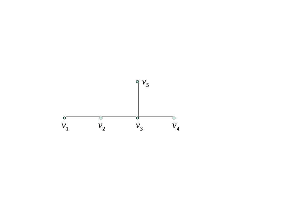
Figure 1. A chemical tree $G$ on vertex set $V(G)=\{v_{1},v_{2},\cdots,v_{5}\}$. Recall that a chemical tree is a tree having no vertex with degree greater than 4.

Example 2. In Fig. 1 we display a chemical tree of $n=5$ vertices. The distance matrix is

$$D(G)=\left(\begin{array}[]{ccccc}0&1&2&3&3\\ 1&0&1&2&2\\ 2&1&0&1&1\\ 3&2&1&0&2\\ 3&2&1&2&0\end{array}\right).$$

The $D$-eigenvalues of the graph are as follows: $\mu_{1}=7.46,\mu_{2}=-0.51,\mu_{3}=-1.08,\mu_{4}=-2$ and $\mu_{5}=-3.86$. We obtain $DEE(G)=1738.2$.

On the other hand, we can easily obtain $W(G)=18$, $M(G)=7.04$ and $\Delta(G)=3$. Hence, from Theorem 1 we have the following bounds

$$1393.4\leq DEE(G)\leq 32611.7.$$

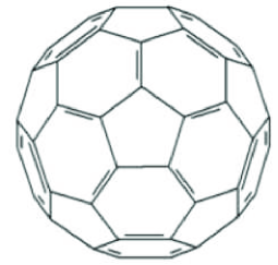
Figure 2. A projection depiction of the buckminsterfullerene $C_{60}$.

Example 3. In this example, we consider the buckminsterfullerene $C_{60}$, which is a well-known member of the fullerene family [15]. As a graph, $C_{60}$ is a truncated icosahedron with $n=60$ vertices and 32 faces (including 20 hexagons and 12 pentagons); see Fig. 2 for an illustration. The $D$-eigenvalues of $C_{60}$ were computed in [1] by using the Givens-Householder method (see Table 1 in [1]). For example, there are exactly 18 positive $D$-eigenvalues and no zero $D$-eigenvalue. Based on these $D$-eigenvalues we calculate by definition (1) that $DEE(C_{60})=152.11+e^{278}$.

Since $C_{60}$ contains 60 vertices, a wise approach to capture its distance matrix is to understand the associated distance level diagram, as is done in Figure 1 of [1]. From that, we conclude that $C_{60}$ is a connected $r$-distance regular graph with $r=278$ and the diameter is $\Delta(C_{60})=9$. Hence, $W(C_{60})=nr/2=8340$ and $M(C_{60})=r=278$. Corollary 1 leads to the following bounds

$$0.53+e^{278}\leq DEE(C_{60})\leq 59+e^{387}.$$

Clearly, the upper bound obtained is way above the true value for $DEE(C_{60})$. Future work may study better behaved estimations.

References

• [1] K. Balasubramanian, A topological analysis of the $C_{60}$ buckminsterfullerene and $C_{70}$ based on distance matrices. Chem. Phys. Lett., 239(1995) 117–123
• [2] R. B. Bapat, S. Sivasubramanian, Product distance matrix of a graph and squared distance matrix of a tree. Appl. Anal. Discrete Math., 7(2013) 285–301
• [3] Ş. B. Bozkurt, C. Adiga, D. Bozkurt, Bounds on the distance energy and the distance Estrada index of strongly quotient graphs. J. Appl. Math., 2013(2013) Art. no. 681019
• [4] Ş. B. Bozkurt, D. Bozkurt, Bounds for the distance Estrada index of graphs. Available at arXiv:1205.1189
• [5] D. M. CvetkoviΔ‡, M. Doob, H. Sachs, Spectra of Graphs: Theory and Application. Johann Ambrosius Bart Verlag, Heidelberg, 1995
• [6] K. C. Das, S.-G. Lee, On the Estrada index conjecture. Linear Algebra Appl., 431(2009) 1351–1359
• [7] J. A. de la PeΓ±a, I. Gutman, J. Rada, Estimating the Estrada index. Linear Algebra Appl., 427(2007) 70–76
• [8] A. A. Dobrynin, R. Entringer, I. Gutman, Wiener index of trees: theory and applications. Acta Appl. Math., 66(2001) 211–249
• [9] E. Estrada, Characterization of 3D molecular structure. Chem. Phys. Lett., 319(2000) 713–718
• [10] E. Estrada, Characterization of the folding degree of proteins. Bioinformatics, 18(2002) 697–704
• [11] E. Estrada, Characterization of the amino acid contribution to the folding degree of proteins. Proteins, 54(2004) 727–737
• [12] E. Estrada, J. A. RodrΓ­guez-VelΓ‘zquez, Spectral measures of bipartivity in complex networks. Phys. Rev. E, 72(2005) 046105
• [13] A. D. GΓΌngΓΆr, Ş. B. Bozkurt, On the distance Estrada index of graphs. Hacettepe J. Math. Stat., 38(2009) 277–283
• [14] I. Gutman, H. Deng, S. RadenkoviΔ‡, The Estrada index: an updated survey. In: D. CvetkoviΔ‡, I. Gutman (Eds.), Selected Topics on Applications of Graph Spectra, Math. Inst., Beograd, 2011, 155–174
• [15] H. W. Kroto, J. R. Heath, S. C. O’Brien, R. F. Curl, R. E. Smalley, $C_{60}$: Buckminsterfullerene. Nature, 318(1985) 162–163
• [16] T. Hilano, K. Nomura, Distance degree regular graphs. J. Comb. Theory Ser. B, 37(1984) 96–100
• [17] A. IliΔ‡, D. StevanoviΔ‡, The Estrada index of chemical trees. J. Math. Chem., 47(2010) 305–314
• [18] G. Indulal, Sharp bounds on the distance spectral radius and the distance energy of graphs. Linear Algebra Appl., 430(2009) 106–113
• [19] G. Indulal, I. Gutman, On the distance spectra of some graphs. Math. Commun., 13(2008) 123–131
• [20] S. NikoliΔ‡, N. TrinajstiΔ‡, Z. MihaliΔ‡, The Wiener index: development and applications. Croat. Chem. Acta, 68(1995) 105–129
• [21] M. RandiΔ‡, In search for graph invariants of chemical interest. J. Mol. Struct., 300(1993) 551–571
• [22] Y. Shang, Distance Estrada index of random graphs. Linear and Multilinear Algebra, DOI:10.1080/03081087.2013.872640
• [23] Y. Shang, Perturbation results for the Estrada index in weighted networks. J. Phys. A: Math. Theor., 44(2011) 075003
• [24] Y. Shang, Lower bounds for the Estrada index using mixing time and Laplacian spectrum. Rocky Mountain J. Math., 43(2013) 2009–2016
• [25] Y. Shang, Estrada index of general weighted graphs. Bull. Aust. Math. Soc., 88(2013) 106–112
• [26] H. B. Walikar, V. S. Shigehalli, H. S. Ramane, Bounds on the Wiener number of a graph. MATCH Comm. Math. Comp. Chem., 50(2004) 117–132
• [27] H. Wiener, Structural determination of paraffin boiling points. J. Amer. Chem. Soc., 69(1947) 17–20
• [28] B. Zhou, On Estrada index. MATCH Comm. Math. Comp. Chem., 60(2008) 485–492
• [29] B. Zhou, I. Gutman, T. AleksiΔ‡, A note on Laplacian energy of graphs. MATCH Comm. Math. Comp. Chem., 60(2008) 441–446