Curvature Motion in a Minkowski Plane

Abstract.

In this paper we study the curvature flow of a curve in a plane endowed with a minkowskian norm whose unit ball is smooth. We show that many of the properties known in the euclidean case can be extended (with due adaptations) to this new situation. In particular, we show that simple, closed, strictly convex, smooth curves remain so until the area enclosed by them vanishes. Moreover, their isoperimetric ratios converge to the minimum possible value, only attained by the minkowskian circle – so these curves converge to a minkowskian ”circular point” as the enclosed area approaches zero.

1. Introduction

Note: Since we wrote this paper, it came to our attention that its main results have already been published. See:

[1] Gage, M., Evolving plane curves by curvature in relative geometries, Duke Math J. 72 (1993) 441-466.
[2] Gage, M. & Li, Y., Evolving plane curves by curvature in relative geometries II, Duke Math J. 75 (1994) 79-98.

Possibly the most fascinating front deformation, the classical planar Curvature Motion is defined by

$$\frac{\partial\gamma}{\partial t}\left(u,t\right)=k\left(u,t\right)N\left(u,t\right)$$

where $k$ and $N$ are the curvature and the inwards unit normal vector to the closed curve $\gamma\left(\cdot,t\right)$ at the point $\gamma\left(u,t\right)$. A series of papers ([3], [4], [5] and [6]) has shown that any embedded curve in the Euclidean plane remains embedded and converges to a ”circular point” in finite time. Moreover, if $L\left(t\right)$ and $A\left(t\right)$ are the length of $\gamma$ and the area it encloses, some very simple formulae can be shown about their evolutions:

$$\frac{dL}{dt} =-\int k^{2}ds$$

$$\frac{dA}{dt} =-2\pi$$

$$\lim_{t\rightarrow t_{V}}\frac{L^{2}}{A} =4\pi$$

(where $t_{V}=\frac{A\left(0\right)}{2\pi}$) the last one being one interpretation of ”converging to a circular shape”.

On the other hand, a Minkowski plane is a 2-dimensional vector space with a norm which can be defined by its unit ball $\mathcal{P}$ (a convex symmetric set). Of course, along with a different geometry, come different notions of lengths, normal vectors and curvature, which we very briefly review in the next section (see [12] for details and [7], [8] for a survey). So it is natural to ask: are the properties of Curvature Motion still valid on the Minkowski plane, with the due adaptations? The goal of this paper is to answer a resounding YES, at least when the boundary of $\mathcal{P}$ is smooth and the initial curve $\gamma\left(\cdot,0\right)$ is smooth and strictly convex. More specifically, following similar techniques as in [3], [4] and [5], we show that the flow is well defined up to the vanishing time $t_{V}=\frac{A\left(\gamma\left(0\right)\right)}{2A\left(\mathcal{P}\right)}$, and that

$$\frac{dL_{\mathcal{Q}}}{dt} = -\int k^{2}ds$$

$$\frac{dA}{dt} = -2A\left(\mathcal{P}\right)$$

$$\lim_{t\rightarrow t_{V}}\frac{L_{\mathcal{Q}}^{2}}{A} = 4A\left(\mathcal{P}\right)$$

where $A\left(\mathcal{P}\right)$ is the area of the unit ball $\mathcal{P}$ and all lengths are taken with respect to the metric defined by the dual unit ball $\mathcal{Q}$.

The structure of this paper is as follows: section 2 briefly reminds us of the basic ideas of Minkowski plane geometry, including some notation choices. Section 3 states many interesting and necessary minkowskian isoperimetric inequalities; it is divided in two subsections, the first devoted to the minkowskian version of Gage´s inequality and the second to a lemma with a more technical proof. Section 4 defines the Minkowskian curvature flow and calculates the evolutions of curvatures, lengths and areas as long as the flow is well defined. Section 5 shows the convergence of the isoperimetric ratio to the ”circular” value $4A\left(\mathcal{P}\right)$ if the enclosed area goes to $0$ and the curves remain simple and convex along the motion. Finally, the technical section 6 has the job of showing the existence of such a flow, all the way until the enclosed area converges to $0$, at least when the initial curve is strictly convex and smooth, rounding up the former results.

Acknowledgment. The authors would like to thank CNPq for financial support during the preparation of this manuscript.

2. Minkowski plane and its dual

Let $\mathcal{P}$ be a strictly convex set, symmetric (which, throughout the paper, will mean ”symmetric with respect to the origin”), whose boundary is given by a $C^{\infty}$ curve $p$. We endow the plane $\mathbb{R}^{2}$ with a norm which makes $\mathcal{P}$ the unit ball. In other words, given $v\in\mathbb{R}^{2}$, write $v=tp$ for some $t\geq 0$ and some $p$ in the boundary of $\mathcal{P}$, and define $||v||_{\mathcal{P}}=t$.

Denoting $e_{r}=(\cos\theta,\sin\theta)$ and $e_{\theta}=(-\sin\theta,\cos\theta)$ we parameterize $p$ by $p(\theta)$, $0\leq\theta\leq 2\pi$, such that $p^{\prime}(\theta)$ is a non-negative multiple of $e_{\theta}$, i.e., the angle between the $x$-axis and $p^{\prime}\left(\theta\right)$ is $\theta+\pi/2$. We can write

(2.1) $$p(\theta) =a(\theta)e_{r}+a^{\prime}(\theta)e_{\theta}$$

$$p^{\prime}\left(\theta\right) =\left(a\left(\theta\right)+a^{\prime\prime}\left(\theta\right)\right)e_{\theta}$$

$$\left[p,p^{\prime}\right] =a\left(\theta\right)\left(a\left(\theta\right)+a^{\prime\prime}\left(\theta\right)\right)$$

where $a(\theta)$ is the support function of $\mathcal{P}$. Furthermore, we shall assume $a(\theta)+a^{\prime\prime}(\theta)>0$ for each $0\leq\theta\leq 2\pi$, which is equivalent to say that the curvature of $p$ is strictly positive.

The dual unity ball $\mathcal{P}^{\ast}$ can be naturally identified with a convex set $\mathcal{Q}$ in the plane with $p^{\ast}(w)=[w,q]$ for any $w\in\mathbb{R}^{2}$. One can see that

(2.2) $$q(\theta) = \frac{p^{\prime}(\theta)}{[p(\theta),p^{\prime}(\theta)]}=\frac{1}{a\left(\theta\right)}e_{\theta}$$

$$q^{\prime}\left(\theta\right) = -\frac{1}{a\left(\theta\right)}e_{r}-\frac{a^{\prime}\left(\theta\right)}{a^{2}\left(\theta\right)}e_{\theta}$$

$$\left[q,q^{\prime}\right] = a^{-2}\left(\theta\right)$$

is a parameterization of the boundary of $\mathcal{Q}$. It is not difficult to see that $q$ is a convex symmetric curve with strictly positive curvature as well. It also holds that

(2.3) $$p(\theta)=-\frac{q^{\prime}(\theta)}{[q(\theta),q^{\prime}(\theta)]}=-a^{2}q^{\prime}\left(\theta\right)$$

Given another closed, strictly convex curve $\gamma$, we can parameterize it by $\theta$ such that $\gamma^{\prime}(\theta)=\lambda(\theta)q(\theta)$ (in fact, anytime we use the notation $f^{\prime}$ we mean derivative with respect to this parameter $\theta$). The Minkowski $\mathcal{Q}$-length $L_{\mathcal{Q}}$ of $\gamma$ is defined as

$$L_{\mathcal{Q}}(\gamma)=\int_{0}^{2\pi}\lambda(\theta)\ d\theta$$

which inspires another useful parameterization of $\gamma$ by its $\mathcal{Q}$-arclength parameter $s$:

$$s\left(\theta\right)=\int_{0}^{\theta}\lambda\left(\sigma\right)d\sigma$$

Sometimes we will need a third different parameterization $\gamma\left(u\right)$ for such a curve. In that case, we define $v=\frac{ds}{du}$ so we can write

$$ds=vdu=\lambda d\theta$$

If a $\mathcal{P}$-circle is tangent to $\gamma$ at $\gamma\left(\theta\right)$, the line joining its center to $\gamma\left(\theta\right)$ must be parallel to $p\left(\theta\right)$. Thus, it is natural to define the minkowskian unit normal to the curve $\gamma$ at the point $\gamma(\theta)$ as $p(\theta)$. The inverse of the radius of a $\mathcal{P}$-circle which has a $3$-point contact with $\gamma$ at $\gamma\left(\theta\right)$ is the minkowskian curvature

(2.4) $$k(\theta)=\left[p,p^{\prime}\right]\frac{d\theta}{ds}=\frac{[p,p^{\prime}]}{\lambda(\theta)}.$$

Other notions of minkowskian curvature are possible – in [10] $k\left(\theta\right)$ is called ”circular curvature” (see also [1] and [11]).

Define the support function $f:[0,2\pi]\rightarrow\mathbb{R}$ of $\gamma$ by $f(\theta)=[\gamma(\theta),q(\theta)]$. Notice that we can take $f$ naturally on the parameter $s$. We have

Proposition 2.1.

The following equalities hold:

(a):

$\displaystyle\int_{0}^{L_{\mathcal{Q}}}k(s)ds=2A(\mathcal{P})$;

(b):

$\displaystyle\int_{0}^{L_{\mathcal{Q}}}f(s)ds=2A$; and

(c):

$\displaystyle\int_{0}^{L_{\mathcal{Q}}}f(s)k(s)ds=L_{\mathcal{Q}}$

Proof.

Since $ds=\lambda d\theta$, equation (2.4) yields

$$\int_{0}^{L_{\mathcal{Q}}}k(s)ds=\int_{0}^{2\pi}k(\theta)\lambda(\theta)d\theta=\int_{0}^{2\pi}[p(\theta),p^{\prime}(\theta)]d\theta=2A(\mathcal{P})$$

and this proves (a). For (b) we calculate

$$\int_{0}^{L_{\mathcal{Q}}}f(s)ds=\int_{0}^{2\pi}[\gamma(\theta),q(\theta)]\lambda(\theta)d\theta=\int_{0}^{2\pi}[\gamma(\theta),\gamma^{\prime}(\theta)]d\theta=2A$$

Now, for (c),

$$\int_{0}^{L_{\mathcal{Q}}}f(s)k(s)ds =\int_{0}^{2\pi}[\gamma(\theta),q(\theta)]k(\theta)\lambda(\theta)d\theta=\int_{0}^{2\pi}[\gamma(\theta),q(\theta)][p(\theta),p^{\prime}(\theta)]d\theta=$$

$$=\int_{0}^{2\pi}[\gamma(\theta),p^{\prime}(\theta)]d\theta=\int_{0}^{2\pi}[p(\theta),\gamma^{\prime}(\theta)]d\theta=\int_{0}^{2\pi}\lambda(\theta)d\theta=L_{\mathcal{Q}}$$

∎

3. Some Isoperimetric Inequalities

Consider again a smooth, closed and convex curve $\gamma$ with $\mathcal{Q}$-length $L_{\mathcal{Q}}$ enclosing the (usual) area $A$. The following isoperimetric inequality generalizes the classical euclidean one (see Cap.4 of [12]):

(3.1) $$\frac{L_{\mathcal{Q}}^{2}}{A}\geq 4A(\mathcal{P}),$$

where $A(\mathcal{P})$ is the usual area of the unit $\mathcal{P}$-ball. As in the euclidean case, the equality holds if and only if the curve is the boundary of some $\mathcal{P}$-ball.

3.1. The Minkowskian Gage Inequality

We now turn our attention to prove a version of the Gage’s inequality (see [3]) in the Minkowski plane. Let $\mathcal{C}$ be the space of smooth, simple, closed and strictly convex curves in the plane endowed with the Hausdorff topology. We have:

Theorem 3.1.

There exists a non-negative, continuous, scale-invariant functional $F:\mathcal{C}\rightarrow\mathbb{R}$ such that

$$\left(1-F(\gamma)\right)\int_{0}^{L_{\mathcal{Q}}}k^{2}ds-A(\mathcal{P})\frac{L_{\mathcal{Q}}}{A}\geq 0,$$

where $A$, $L_{\mathcal{Q}}$ and $k$ are the area, $\mathcal{Q}$-length and curvature of $\gamma$. Moreover $F\left(\gamma\right)=0$ if and only if $\gamma$ is a $\mathcal{P}$-circle.

Corollary 3.1.

Given $\gamma\in\mathcal{C}$, we have

(3.2) $$\int_{0}^{L_{\mathcal{Q}}}k^{2}ds-A(\mathcal{P})\frac{L_{\mathcal{Q}}}{A}\geq 0.$$

with equality if and only if $\gamma$ is a $\mathcal{P}$-circle.

In order to prove this, we need many results. We start by recalling an useful Bonnesen inequality whose proof can be found in Theorem 4.5.5 of [12]:

Theorem 3.2.

For $\gamma\in\mathcal{C}$, let $r_{\mathrm{in}}$ be the radius of the biggest inscribed $\mathcal{P}$-circle and $r_{\mathrm{out}}$ the radius of the smallest circumscribed $\mathcal{P}$-circle. Then

(3.3) $$rL_{\mathcal{Q}}-A-A(\mathcal{P})r^{2}\geq 0$$

whenever $r_{\mathrm{in}}\leq r\leq r_{\mathrm{out}}$.

Lemma 3.1.

The equality in (3.3) holds for $r=r_{\mathrm{in}}$ if and only if $\gamma$ is homothetic to the $\mathcal{P}$-circle.

We have not seen a proof of this lemma in the literature, so we prove it in the next subsection. Now let us begin to build the functional $F\left(\gamma\right)$ of Gage´s inequality:

Proposition 3.1.

Consider the space $\mathcal{C}_{s}$ consisting of curves in $\mathcal{C}$ which are symmetric. Define the functional $E:\mathcal{C}_{s}\rightarrow\mathbb{R}$ by

$$E(\gamma)=1+\frac{A(\mathcal{P})r_{\mathrm{in}}r_{\mathrm{out}}}{A}-\frac{2A(\mathcal{P})(r_{\mathrm{in}}+r_{\mathrm{out}})}{L_{\mathcal{Q}}}$$

Then, the following hold:
(1) $L_{\mathcal{Q}}A\left(1-E(\gamma)\right)\geq A(\mathcal{P})\displaystyle\int_{0}^{L_{\mathcal{Q}}}f^{2}ds$, for all $\gamma\in\mathcal{C}_{s}$;
(2) $E(\gamma)\geq 0$ and equality holds if and only if $\gamma$ is a $\mathcal{P}$-circle; and
(3) If $\gamma_{j}$ is a sequence in $\mathcal{C}_{s}$ such that $\displaystyle\lim_{j\rightarrow\infty}E(\gamma_{j})=0$ and if the sequence of the normalized curves $\eta_{j}=\gamma_{j}\displaystyle\sqrt{\frac{A(\mathcal{P})}{A}}$ is contained in some bounded region of the plane, then the region $H_{j}$ enclosed by $\eta_{j}$ converges in the Hausdorff metric to $\mathcal{P}$, as $j\rightarrow\infty$.

Proof.

If $r_{\mathrm{in}}\leq r\leq r_{\mathrm{out}}$ then

$$\left(r-r_{\mathrm{in}}\right)\left(r_{\mathrm{out}}-r\right)\geq 0\Rightarrow r\left(r_{\mathrm{in}}+r_{\mathrm{out}}\right)-r_{\mathrm{in}}r_{\mathrm{out}}\geq r^{2}$$

For a curve $\gamma$ in $\mathcal{C}_{s}$ the support function $f$ satisfies $r_{\mathrm{in}}\leq f\leq r_{\mathrm{out}}$ for every value of the parameter, so we can take $r=f$ above. Then we integrate the above inequality to obtain

$$\left(r_{\mathrm{out}}+r_{\mathrm{in}}\right)\int_{0}^{L_{\mathcal{Q}}}f\ ds-r_{\mathrm{in}}r_{\mathrm{out}}L_{\mathcal{Q}}\geq\int_{0}^{L_{\mathcal{Q}}}f^{2}ds$$

Since $\displaystyle\int_{0}^{L_{\mathcal{Q}}}f\ ds=2A$ we have the inequality in (1). For (2) let $g\left(r\right)=rL_{\mathcal{Q}}-A-A(\mathcal{P})r^{2}.$ From Theorem 3.2.we know that $g\left(r_{\mathrm{in}}\right),g\left(r_{\mathrm{out}}\right)\geq 0,$ so we may write for $r\in\left[r_{\mathrm{in}},r_{\mathrm{out}}\right]$

$$\frac{r-r_{\mathrm{in}}}{r_{\mathrm{out}}-r_{\mathrm{in}}}g\left(r_{\mathrm{out}}\right)+\frac{r_{\mathrm{out}}-r}{r_{\mathrm{out}}-r_{\mathrm{in}}}g\left(r_{\mathrm{in}}\right)\geq 0$$

which can be rewritten as

$$r\left(L_{\mathcal{Q}}-A\left(\mathcal{P}\right)\left(r_{\mathrm{out}}+r_{\mathrm{in}}\right)\right)-A+A\left(\mathcal{P}\right)r_{\mathrm{in}}r_{\mathrm{out}}\geq 0.$$

Taking $r=f$ and integrating with respect to $s$

$$2A\left(L_{Q}-A\left(P\right)\left(r_{\mathrm{out}}+r_{\mathrm{in}}\right)\right)-AL_{\mathcal{Q}}+A\left(\mathcal{P}\right)r_{\mathrm{in}}r_{\mathrm{out}}L_{\mathcal{Q}}\geq 0$$

which shows that $E\left(\gamma\right)\geq 0$. Since $f$ ranges from $r_{\mathrm{in}}$ to $r_{\mathrm{out}}$, if $E(\gamma)=0$ then we must have $g\left(r_{\mathrm{in}}\right)=g\left(r_{\mathrm{out}}\right)=0$ and Lemma 3.1 says that $\gamma$ is a $\mathcal{P}-$circle.

For (3) let $\gamma_{j}$ be a sequence in $\mathcal{C}_{s}$ such that $\displaystyle\lim_{j\rightarrow\infty}E(\gamma_{j})=0$ and assume that all normalized curves $\eta_{j}$ lie at a same bounded region of the plane. Notice that $E(\eta_{j})=E(\gamma_{j})$ for every $j\in\mathbb{N}$ and then $\displaystyle\lim_{j\rightarrow\infty}E(\eta_{j})=0$. Denote by $H_{j}$ the region enclosed by $\eta_{j}$. By Blaschke’s Selection Theorem we have that there exists a subsequence $H_{j_{k}}$ which converges to a convex set $H$. Since $E$ is a continuous functional (considering the Hausdorff topology in $\mathcal{C}_{s}$) we have $E(H)=\displaystyle\lim_{k\rightarrow\infty}E(H_{j_{k}})=0$, and then $H$ must be the unit $\mathcal{P}$-circle. It is also true that every convergent subsequence of $H_{j}$ converges to the unit $\mathcal{P}$-circle. It follows immediately that $H_{j}$ itself converges to the unit $\mathcal{P}$-circle. This concludes the proof. ∎

Finally we appropriately extend the functional $E$ to the desired functional $F$, as done in [4]. Let $\gamma\in\mathcal{C}$, and consider all chords which divide the area inside $\gamma$ in two equal parts. Pick one (call it $S$) such that the tangent lines to $\gamma$ on the extreme points are parallel. Let $\gamma_{1}$ (with $\mathcal{Q}$-length $L_{1}$) and $\gamma_{2}$ (with $\mathcal{Q}$-length $L_{2}$) be the two portions of $\gamma$ determined by $S$. Placing the $x$-axis along $S$ and the origin at its midpoint we can build two curves $\gamma_{1}^{\ast}$ and $\gamma_{2}^{\ast}$ which belongs to $\mathcal{C}_{s}$ by reflecting $\gamma_{1}$ and $\gamma_{2}$ through the origin. Since the functional $E$ is well defined for these new curves we could define $F(\gamma)$ by

$$F(\gamma)=\frac{L_{1}}{L_{\mathcal{Q}}}E(\gamma_{1}^{\ast})+\frac{L_{2}}{L_{\mathcal{Q}}}E(\gamma_{2}^{\ast}),$$

but, although this definition looks natural (because it coincides with $E$ in $\mathcal{C}_{s}$), it is not always correct. This happens because the choice of the chord $S$ is not necessarily unique. To overcome this trouble we define $F$ to be the supremum of the above expression between all possible choices of $S$. It is not difficult to prove that the functional $F$ has also the properties (1), (2) and (3), and we will omit the details.

Now we can finish the proof of Theorem 3.1. By Schwarz inequality we have

$$L_{\mathcal{Q}}=\int_{0}^{L_{\mathcal{Q}}}fk\ ds\leq\left(\int_{0}^{L_{\mathcal{Q}}}f^{2}\ ds\right)^{1/2}\left(\int_{0}^{L_{\mathcal{Q}}}k^{2}ds\right)^{1/2}$$

Squaring both sides and using inequality expressed in Theorem 3.1 yields

$$L_{\mathcal{Q}}^{2}\leq\left(\int_{0}^{L_{\mathcal{Q}}}f^{2}\ ds\right)\left(\int_{0}^{L_{\mathcal{Q}}}k^{2}ds\right)\leq\frac{L_{\mathcal{Q}}A}{A(\mathcal{P})}\left(1-F(\gamma)\right)\int_{0}^{L_{\mathcal{Q}}}k^{2}ds$$

and the desired result comes immediately.

3.2. Proof of Lemma 3.1

Assume that $\gamma\in{\mathcal{C}}$ is symmetric. We start with the following quite intuitive result:

Lemma 3.2.

Denote by $\mu_{0}$ the minimum curvature radius of $\gamma$. Then $\mu_{0}\leq r_{\mathrm{in}}$ with equality only in case $\gamma$ is a $\mathcal{P}$-circle.

Proof.

Assume that $\mu(0)=\mu_{0}$, where $\mu_{0}=\min\{\mu(\theta)|0\leq\theta\leq 2\pi\}$. We may also assume that $(-a,a)$, $0\leq a<\frac{\pi}{2}$, is the maximal interval where $\mu(\theta)=\mu_{0}$. Observe that if $a=\frac{\pi}{2}$ then, by the symmetry of $\gamma$, $\gamma$ would necessarily be a $\mathcal{P}$-circle.

For any $-\pi\leq\theta\leq\pi$, denote $P_{0}=(x_{0}(\theta),y_{0}(\theta))$ the $\mathcal{P}$-circle of radius $\mu_{0}$ osculating at $\gamma(0)$. In the euclidean case, $x_{0}=\mu_{0}\sin(\theta)$, $y_{0}=\mu_{0}-\mu_{0}\cos(\theta)$. Denote also $\gamma(\theta)=(x(\theta),y(\theta))$, $q(\theta)=(q_{1}(\theta),q_{2}(\theta))$ and $p(\theta)=(p_{1}(\theta),p_{2}(\theta))$. Since

$$\gamma^{\prime}(\theta)=\mu(\theta)[p,p^{\prime}](\theta)q(\theta),$$

we can write

$$y(\theta)=\int_{0}^{\theta}\mu[p,p^{\prime}]q_{2}d\theta\geq\mu_{0}\left(p_{2}(\theta)-p_{2}(0)\right)=y_{0}(\theta),$$

with equality if and only if $-a\leq\theta\leq a$. We conclude that $y(\theta)\geq y_{0}(\theta)$, and the equality holds if and only if $-a\leq\theta\leq a$. Thus the osculating $\mathcal{P}$-circle $P_{0}$ is tangent to $\gamma$ only at $\gamma(\theta)$, $-a\leq\theta\leq a$. So there exists $\epsilon>0$ such that $P_{0}+(0,\epsilon)$ is contained in the interior of $\gamma$, thus proving the proposition. ∎

For $0\leq r\leq r_{\mathrm{in}}$, denote $D_{r}$ the set of points inside $\gamma$ whose distance to $\gamma$ is $\geq r$ and let $C_{r}=\partial D_{r}$. Denote by $L_{\mathcal{Q}}(r)$ the $\mathcal{Q}$-length of $C_{r}$. The following proposition is easy to prove:

Proposition 3.2.

If $r\leq\mu_{0}$, then

(3.4) $$L_{\mathcal{Q}}(r)=L_{\mathcal{Q}}-2A(\mathcal{P})r.$$

Moreover,

(3.5) $$A=\int_{0}^{r_{\mathrm{in}}}L_{\mathcal{Q}}(r)dr.$$

Proof.

Let

$$\beta(\theta,r)=\gamma(\theta)-rp(\theta)$$

be a parameterization of $C_{r}$, $\theta\in I(r)$. If $r<\mu_{0}$, then $I(r)=[0.2\pi]$ and so

$$L_{\mathcal{Q}}(r)=\int_{0}^{2\pi}[p,p^{\prime}](\mu(\theta)-r)d\theta=L_{\mathcal{Q}}(0)-2A(P)r,$$

which proves equation (3.4). To prove equation (3.5), observe that the region $D$ enclosed by $\gamma$ is the disjoint union of $C_{r}$, $0\leq r\leq r_{\mathrm{in}}$. Since

$$\left[\frac{\partial\beta}{\partial\theta},\frac{\partial\beta}{\partial r}\right]=[p,p^{\prime}]\left(\mu(\theta)-r\right).$$

and $\mu(\theta)-r>0$, for $\theta\in I(r)$, we conclude that

$$A=\int_{r=0}^{r_{in}}\int_{I(r)}[p,p^{\prime}]\left(\mu(\theta)-r\right)d\theta dr=\int_{r=0}^{r_{in}}L_{\mathcal{Q}}(r)dr.$$

∎

Now consider an arc of the unit $\mathcal{P}$-circle defined by $\theta_{1}\leq\theta\leq\theta_{2}$. Taking the tangents to $\mathcal{P}$ at $\theta=\theta_{1}$ and $\theta=\theta_{2}$ we obtain a polygonal line formed by a pair of segments (see Figure 3.1). It is not difficult to verify that the $Q$-lengths of the segments are

(3.6) $$L_{1}=\frac{1-[p(\theta_{1}),q(\theta_{2})]}{[q(\theta_{1}),q(\theta_{2})]};\ \ L_{2}=\frac{1-[p(\theta_{2}),q(\theta_{1})]}{[q(\theta_{1}),q(\theta_{2})]}.$$

The $Q$-length of the arc is given by

(3.7) $$L_{arc}=\int_{\theta_{1}}^{\theta_{2}}[p,p^{\prime}]d\theta,$$

and we define

(3.8) $$\delta(\theta_{1},\theta_{2})=L_{1}+L_{2}-L_{arc}.$$

Then $\delta=\delta(\theta_{1},\theta_{2})$ is strictly positive (see [12]).

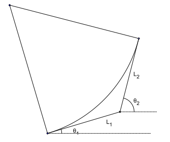
Figure 3.1. Tangent segments to $\mathcal{P}$ at $\theta_{1}$ and $\theta_{2}$.

Figure 3.2. Arcs of $C$ between $\theta_{1}$ and $\theta_{2}$ and $V$.

For $r>\mu_{0}$, the curves $C_{r}$ necessarily admit corners. Thus we must consider curves which are smooth by parts with a finite number of vertices.

Lemma 3.3.

Assume that $C$ is smooth by parts and at some corner $V$ the parameter of the tangent lines are $\theta_{1}$ and $\theta_{2}$. Consider an arc of $\mathcal{P}$-circle of radius $z$ inscribed in this corner. Denote by $l_{1}(z)$ and $l_{2}(z)$ the $Q$-lengths of the arcs of $C$ between the vertex $V$ and the tangency points $P_{1}\left(z\right)$ and $P_{2}\left(z\right)$(see Figure 3.2). Then

$$l_{1}(z)+l_{2}(z)=zL_{arc}+z\delta\left(\theta_{1},\theta_{2}\right)+O(z^{2}),$$

where $\lim_{z\rightarrow 0}\frac{O(z^{2})}{z}=0.$

Proof.

We parameterize $C$ around $V$ by an $\mathcal{Q}$-arclength parameter $s$ using a function $g:\left(-\varepsilon,\varepsilon\right)\rightarrow\mathbb{R}^{2}$ with $g\left(0\right)=V$ (so $g$ is smooth everywhere except at $s=0$, where we have lateral derivatives

$$\frac{dg}{ds}\left(0_{-}\right)=q\left(\theta_{1}\right)\ \mathrm{and}\ \frac{dg}{ds}\left(0_{+}\right)=q\left(\theta_{2}\right)$$

The definition of the tangent points means that $P_{1}\left(z\right)=g\left(-l_{1}\left(z\right)\right)$ and $P_{2}\left(z\right)=g\left(l_{2}\left(z\right)\right)$. Writing the position of the center $O\left(z\right)$ in two ways, we write $l_{1}$ and $l_{2}$ implicitly as a function of $z$:

$$g\left(-l_{1}\left(z\right)\right)-zp\left(\theta_{1}\left(z\right)\right)=g\left(l_{2}\left(z\right)\right)-zp\left(\theta_{2}\left(z\right)\right)$$

where $\theta_{1}\left(z\right)$ and $\theta_{2}\left(z\right)$ are the $\theta$-parameters associated to $P_{1}$ and $P_{2}$. Take derivatives with respect to $z$ and then take $z\rightarrow 0$ (so $\theta_{1}\left(z\right)\rightarrow\theta_{1}$ and $\theta_{2}\left(z\right)\rightarrow\theta_{2}$) to arrive at

$$-q\left(\theta_{1}\right)\frac{dl_{1}}{dz}\left(0\right)-p\left(\theta_{1}\right)=q\left(\theta_{2}\right)\frac{dl_{2}}{dz}\left(0\right)-p\left(\theta_{2}\right)$$

Now, this equation depends only on the angles $\theta_{1}$ and $\theta_{2}$ – the exact shape of $C$ does not matter at all! So, up to first order, the lengths $l_{1}$ and $l_{2}$ depend on $z$ the same way they would if the curve were already the polygonal in 3.1 (scaled by a factor of $z$), that is

$$l_{1}\left(z\right)+l_{2}\left(z\right) = z\left(L_{1}+L_{2}\right)+O\left(z^{2}\right)=$$

$$= zL_{arc}+z\delta\left(\theta_{1},\theta_{2}\right)+O\left(z^{2}\right).$$

∎

Proposition 3.3.

Consider a convex curve $C$ with at least one corner. Then

$$\frac{dL_{\mathcal{Q}}}{ds}(0)<-2A(\mathcal{P}).$$

Proof.

Denote $\theta_{1}<\theta_{2}$ the angles of a corner $k$ and consider an arc of the circle $\mathcal{P}$ defined by the angles $\theta_{1}$ and $\theta_{2}$. Consider $z$ small and inscribe a circle $z\mathcal{P}$ at a corner $k$. Denote $\overline{C}_{z}$ the curve obtained from $C$ by substituting each corner by the corresponding arc of the circle $z\mathcal{P}$. By Lemma 3.3, the length difference at the corner $k$ is $l_{k}(C)-L_{k}(\overline{C}_{z})=z\delta_{k}+O(z^{2})$. Since

$$L_{\mathcal{Q}}(\overline{C}_{z})=L_{\mathcal{Q}}(z)+2A(\mathcal{P})z,$$

we conclude that

$$L_{\mathcal{Q}}(0)=L_{\mathcal{Q}}(z)+\left(2A(\mathcal{P})+\sum_{k}\delta_{k}\right)z+O(z^{2}),$$

thus proving the proposition. ∎

Corollary 3.2.

If $r>\mu_{0}$ then $L_{\mathcal{Q}}(r)<L_{\mathcal{Q}}-2A(\mathcal{P})r$.

Proof.

By Proposition 3.3, $\frac{dL_{Q}}{ds}\leq-2A(\mathcal{P})$ with equality if and only if $s\leq\mu_{0}$. In fact, $C_{r}$ has a corner if and only if $r>\mu_{0}$. Integrating from $0$ to $r$ we obtain $L_{\mathcal{Q}}(r)<L_{\mathcal{Q}}-2A(\mathcal{P})r$. ∎

Now we can complete the proof of Lemma 3.1: if equality holds in 3.3, then Proposition 3.2 and Corollary 3.2 imply that $r_{\mathrm{in}}\leq\mu_{0}$. But then Lemma 3.2 implies that $r_{\mathrm{in}}=\mu_{0}$ and $\gamma$ is a $P$-circle.

Remark. Lemma 3.1 is not necessarily true if $\gamma$ and the $\mathcal{P}$-ball are not smooth! A counterexample: take $\mathcal{P}$ to be the square whose vertices are $(\pm 1,\pm 1)$ (so $\mathcal{Q}$ will be the square $\left|x\right|+\left|y\right|\leq 1$) and $\gamma$ to be the rectangle with vertices $(\pm 2,\pm 1)$.

4. The minkowskian curvature flow

We define the minkowskian curvature flow to be a family of closed curves $F:S^{1}\times[0,T)\rightarrow\mathbb{R}^{2}$ satisfying the following:

(4.1) $$\frac{\partial F}{\partial u}(u,t) =v(u,t).q(\theta(u,t));\ \mathrm{and}$$

$$\frac{\partial F}{\partial t}(u,t) =-k(u,t).p(\theta(u,t))$$

$$F\left(u,0\right) =\gamma\left(u\right)$$

where $\gamma$ is a simple closed curve and, as usual, $\theta(u,t)$ is defined such that the angle between the $x$-axis and $\partial F/\partial u$ at the point $(u,t)$ is $\theta(u,t)+\pi/2$.

Lemma 4.1.

The following hold at each point of the flow:

(a):

$\displaystyle\frac{\partial v}{\partial t}=-k^{2}v$; and

(b):

$\displaystyle\frac{\partial\theta}{\partial t}=\frac{1}{v\left[q,q^{\prime}\right]}\frac{\partial k}{\partial u}=\frac{1}{\left[q,q^{\prime}\right]}\frac{\partial k}{\partial s}$

Proof.

Notice first that

$$\frac{\partial}{\partial t}\left(\frac{\partial F}{\partial u}\right)=\frac{\partial v}{\partial t}.q+v\frac{\partial\theta}{\partial t}.q^{\prime}=\frac{\partial v}{\partial t}.q-v\frac{\partial\theta}{\partial t}[q,q^{\prime}].p$$

Now,

$$\frac{\partial}{\partial u}\left(\frac{\partial F}{\partial t}\right)=-\frac{\partial k}{\partial u}.p-k\frac{\partial\theta}{\partial u}.p^{\prime}=-\frac{\partial k}{\partial u}.p-k\frac{v}{\lambda}[p,p^{\prime}].q=-\frac{\partial k}{\partial u}.p-k^{2}v.q$$

Then the result follows since $p$ and $q$ are always linearly independent. ∎

Lemma 4.2.

The evolutions of the $\mathcal{Q}$-arclength and of the area are given respectively by

$$\frac{dL_{\mathcal{Q}}}{dt}=-\int_{0}^{L_{\mathcal{Q}}(t)}k^{2}(s,t)ds;\ \mathrm{and}$$

$$\frac{dA}{dt}=-2A(\mathcal{P})$$

Proof.

Since $L_{\mathcal{Q}}(t)=\displaystyle\int_{0}^{2\pi}v(u,t)du$ we have

$$\frac{dL_{\mathcal{Q}}}{dt}=\int_{0}^{2\pi}\frac{\partial v}{\partial t}du=-\int_{0}^{2\pi}k^{2}v\ du=-\int_{0}^{L_{\mathcal{Q}}}k^{2}\ ds$$

The area $A(t)$ of the curve at time $t$ is given by

$$\frac{dA}{dt}=\displaystyle\frac{1}{2}\int_{0}^{2\pi}\left[F(u,t),\frac{\partial F}{\partial u}(u,t)\right]du$$

Thus, integrating by parts,

$$\frac{dA}{dt} =\frac{1}{2}\int_{0}^{2\pi}\left[\frac{\partial F}{\partial t},\frac{\partial F}{\partial u}\right]du+\frac{1}{2}\int_{0}^{2\pi}\left[F,\frac{\partial^{2}F}{\partial t\partial u}\right]du=$$

$$=\int_{0}^{2\pi}\left[\frac{\partial F}{\partial t},\frac{\partial F}{\partial u}\right]du=\int_{0}^{2\pi}[-kp,vq]du=$$

$$=\int_{0}^{2\pi}-kv\ du=-\int_{0}^{L_{\mathcal{Q}}}k\ ds=-2A(\mathcal{P})$$

∎

With these evolution formulae one can easily show that the evolution of the isoperimetric ratio is

(4.2) $$\frac{d}{dt}\left(\frac{L_{\mathcal{Q}}^{2}}{A}\right)=-\frac{2L_{\mathcal{Q}}}{A}\left(\int_{0}^{L_{\mathcal{Q}}}k^{2}ds-A(\mathcal{P})\frac{L_{\mathcal{Q}}}{A}\right)$$

which, given (3.2), shows that the isoperimetric ratio is nonincreasing along the motion. In the next section we will prove that, as in the euclidean case, if the flow continues until the area converges to zero and the curves remain simple and convex along the motion, then the isoperimetric ratio converges to the optimum value $4A(\mathcal{P})$. But first, we establish the evolution of the curvature function.

Lemma 4.3.

The minkowskian curvature $k$ evolves according to the PDE

$$\frac{\partial k}{\partial\tau}=\frac{a}{a+a^{\prime\prime}}k^{2}\frac{\partial^{2}k}{\partial\theta^{2}}+\frac{2a^{\prime}}{a+a^{\prime\prime}}k^{2}\frac{\partial k}{\partial\theta}+k^{3},$$

where $\tau$ is the time parameter which is independent with $\theta$.

Proof.

Using Lemma 4.1(a) and $ds=vdu$, we arrive at

$$\frac{\partial}{\partial t}\frac{\partial}{\partial s}-\frac{\partial}{\partial s}\frac{\partial}{\partial t}=k^{2}\frac{\partial}{\partial s}$$

just as in the Euclidean case. We apply this to the function $\theta=\theta(s,t)$ and use $ds=\lambda d\theta$ and Lemma 4.1(b) to obtain

$$\frac{\partial}{\partial t}\left(\frac{k}{[p,p^{\prime}]}\right)-\frac{\partial}{\partial s}\left(\frac{1}{\left[q,q^{\prime}\right]}\frac{\partial k}{\partial s}\right)=\frac{k^{3}}{[p,p^{\prime}]}.$$

Unfortunately $p$ and $q$ now depend on $t$ as well, so, using equations (2.1) and (2.2), we arrive at

$$\frac{1}{a\left(a+a^{\prime\prime}\right)}\frac{\partial k}{\partial t}-\frac{k}{a^{2}\left(a+a^{\prime\prime}\right)^{2}}\left[a^{\prime}\left(a+a^{\prime\prime}\right)+a\left(a^{\prime}+a^{\prime\prime\prime}\right)\right]\frac{\partial\theta}{\partial t}-2aa^{\prime}\frac{\partial k}{\partial s}\frac{\partial\theta}{\partial s}-a^{2}\frac{\partial^{2}k}{\partial s^{2}}=\frac{k^{3}}{a\left(a+a^{\prime\prime}\right)}$$

Now we change all $s$-derivatives to $\theta$-derivatives using equation (2.4), and use Lemma 4.1(b) to eventually get to

$$\frac{\partial k}{\partial t}-\frac{2a^{\prime}}{a+a^{\prime\prime}}k^{2}\frac{\partial k}{\partial\theta}-\frac{a}{a+a^{\prime\prime}}k\left(\frac{\partial k}{\partial\theta}\right)^{2}-\frac{a}{a+a^{\prime\prime}}k^{2}\frac{\partial^{2}k}{\partial\theta^{2}}=k^{3}$$

Now, writing $k=k(\theta,\tau)$ yields

$$\frac{\partial k}{\partial t}=\frac{\partial k}{\partial\theta}\frac{\partial\theta}{\partial t}+\frac{\partial k}{\partial\tau}.$$

Using this (and replacing once again $\displaystyle\frac{\partial\theta}{\partial t}$ using Lemma 4.1(b)) we finish the proof. ∎

5. Convergence of the isoperimetric ratio

We now turn to show that the flow rounds the curves if they approach a vanishing point. In the following $\gamma(u,t):S^{1}\times[0,T)\rightarrow\mathbb{R}^{2}$ is a family (on parameter $t$) of curves in $\mathcal{C}$ which solves the minkowskian curvature flow (in the next section, we will show that $\gamma\left(\cdot,0\right)\in\mathcal{C\Rightarrow\gamma}\left(\cdot,t\right)\in\mathcal{C}$). The $\mathcal{Q}$-length and the area of the curve at time $t$ are denoted, as usual, by $L_{\mathcal{Q}}(t)$ and $A(t)$.

Lemma 5.1.

If $\displaystyle\lim_{t\rightarrow T}A(t)=0$ then

$$\liminf_{t\rightarrow T}L_{\mathcal{Q}}(t)\left(\int_{0}^{L_{\mathcal{Q}}(t)}k^{2}ds-A(\mathcal{P})\frac{L_{\mathcal{Q}}(t)}{A(t)}\right)=0$$

Proof.

Suppose there exist $\epsilon>0$ and $t_{1}\in(0,T)$ such that

$$L_{\mathcal{Q}}(t)\left(\int_{0}^{L_{\mathcal{Q}}(t)}k^{2}ds-A(\mathcal{P})\frac{L_{\mathcal{Q}}(t)}{A(t)}\right)>\epsilon$$

for every $t\in(t_{1},T)$. Put $g(t)=\log(A(t))$ for $t\in[0,T)$. Using the evolution of the isoperimetric ratio (4.2) we have

$$\frac{d}{dt}\left(\frac{L_{\mathcal{Q}}^{2}}{A}\right)\leq-\frac{2}{A}\epsilon=\frac{\epsilon}{A(\mathcal{P})}\frac{dg}{dt}$$

Fix $t\in(t_{1},T)$. Isoperimetric inequality (3.1) and integration (from $t_{1}$ to $t$) yield

$$4A(\mathcal{P})\leq\frac{L_{\mathcal{Q}}^{2}(t)}{A(t)}\leq\frac{L_{\mathcal{Q}}^{2}(t_{1})}{A(t_{1})}-\frac{\epsilon}{A(\mathcal{P})}\log(A(t_{1}))+\frac{\epsilon}{A(\mathcal{P})}\log(A(t))$$

But the right hand side goes to $-\infty$ as $t$ converges to $T$. This contradiction completes the proof. ∎

Now we are ready to prove the main theorem of this section.

Theorem 5.1.

If $\displaystyle\lim_{t\rightarrow T}A(t)=0$ then $\displaystyle\lim_{t\rightarrow T}\frac{L_{\mathcal{Q}}^{2}(t)}{A(t)}=4A(\mathcal{P})$

Proof.

First we rewrite the inequality in Theorem 3.1 as

$$\int_{0}^{L_{\mathcal{Q}}}k^{2}ds-A(\mathcal{P})\frac{L_{\mathcal{Q}}}{A}\geq F(\gamma)\int_{0}^{L_{\mathcal{Q}}}k^{2}ds$$

Schwarz inequality yields

$$L_{\mathcal{Q}}\int_{0}^{L_{\mathcal{Q}}}k^{2}ds\geq\left(\int_{0}^{L_{\mathcal{Q}}}k\ ds\right)^{2}=4A(\mathcal{P})^{2}$$

Combining both inequalities we have the following inequality for each curve $\gamma(\cdot,t)$:

$$L_{\mathcal{Q}}\left(\int_{0}^{L_{\mathcal{Q}}}k^{2}ds-A(\mathcal{P})\frac{L_{\mathcal{Q}}}{A}\right)\geq 4A(\mathcal{P})^{2}F(\gamma)$$

The previous Lemma guarantees that the left hand side converges to $0$ for some subsequence $t_{j}\rightarrow T$. Since $F$ is a non-negative functional we have also $F(t_{j})\rightarrow 0$ as $t_{j}\rightarrow T$. Let $\eta_{j}$ be the normalized curve $\eta_{j}=\displaystyle\sqrt{\frac{A(\mathcal{P})}{A}}\gamma(\cdot,t_{j})$. Using the same technique presented in [4] one can show that the curves $\eta_{j}$ lie in one same bounded region of the plane and then. Since $F$ satisfies property (3) of Theorem 3.1, the region $H_{j}$ enclosed by $\eta_{j}$ converges in the Hausdorff topology to the unit $\mathcal{P}$-disc. It follows that $\displaystyle\frac{L_{\mathcal{Q}}^{2}(t_{j})}{A(t_{j})}$ converges to $4A(\mathcal{P})$ as $t_{j}\rightarrow T$. Since $\displaystyle\frac{L_{\mathcal{Q}}^{2}(t)}{A(t)}$ is nonincreasing the convergence holds, in fact, for every value of the parameter and we have the desired result. ∎

6. Existence of the minkowskian curvature flow

The final step is to prove that the minkowskian curvature flow in fact exists and continues until the area enclosed by the curves converges to zero. We now establish:

Lemma 6.1.

Let $k:[0,2\pi]\rightarrow\mathbb{R}$ be a $C^{1}$ positive $2\pi$-periodic function. Then, $k$ is the Minkowski curvature of a simple closed strictly convex $C^{2}$ plane curve if and only if

(6.1) $$\int_{0}^{2\pi}\frac{a(\theta)+a^{\prime\prime}(\theta)}{k(\theta)}\sin\theta\ d\theta=\int_{0}^{2\pi}\frac{a(\theta)+a^{\prime\prime}(\theta)}{k(\theta)}\cos\theta\ d\theta=0$$

Proof.

Suppose first that $\gamma:[0,2\pi]\rightarrow\mathbb{R}$ is a closed $C^{2}$ curve whose curvature is given by $k$. As $\displaystyle\int_{0}^{2\pi}\gamma^{\prime}(\theta)d\theta=0$ we have

$$0=\int_{0}^{2\pi}\lambda(\theta)q(\theta)d\theta=\int_{0}^{2\pi}\frac{[p(\theta),p^{\prime}(\theta)]}{k(\theta)a(\theta)}(-\sin\theta,\cos\theta)d\theta$$

And then the desired equalities comes from equation 2.1.

On the other hand if $k$ is a $C^{1}$ positive $2\pi$-periodic function such that (6.1) holds we can define

$$\gamma(\theta)=\left(-\int_{0}^{\theta}\frac{a(\sigma)+a^{\prime\prime}(\sigma)}{k(\sigma)}\sin\sigma\ d\sigma,\int_{0}^{\theta}\frac{a(\sigma)+a^{\prime\prime}(\sigma)}{k(\sigma)}\cos\sigma\ d\sigma\right)$$

which is clearly a closed $C^{2}$ curve. Furthermore,

$$\gamma^{\prime}(\theta)=\frac{a(\theta)+a^{\prime\prime}(\theta)}{k(\theta)}(-\sin\theta,\cos\theta)=\frac{a(a+a^{\prime\prime})(\theta)}{k(\theta)}q(\theta)=\frac{[p(\theta),p^{\prime}(\theta)]}{k(\theta)}q(\theta)$$

and then the Minkowski curvature of $\gamma$ is precisely $k$. To complete the proof notice that $\gamma$ is simple as long as its Gauss map is injective. ∎

Now, inspired by Lemma 4.3 we will see how the solution to the curvature motion emerges from the solution of a parabolic differential equation. From now on, we use $t$ for the time parameter which is independent with $\theta$.

Theorem 6.1.

Consider a function $k:S^{1}\times[0,T)\rightarrow\mathbb{R}$, such that $k\in C^{2+\alpha,1+\alpha}(S^{1}\times[0,T-\epsilon])$ for all $\epsilon>0$, satisfying the evolution equation:

(6.2) $$\frac{\partial k}{\partial t}=\frac{a}{a+a^{\prime\prime}}k^{2}\frac{\partial^{2}k}{\partial\theta^{2}}+\frac{2a^{\prime}}{a+a^{\prime\prime}}k^{2}\frac{\partial k}{\partial\theta}+k^{3}$$

with initial value $k(\theta,0)=\varphi(\theta)$ where $\varphi$ is a strictly positive $C^{1+\alpha}$ function such that:

$$\int_{0}^{2\pi}\frac{a(\theta)+a^{\prime\prime}(\theta)}{\varphi(\theta)}\sin\theta\ d\theta=\int_{0}^{2\pi}\frac{a(\theta)+a^{\prime\prime}(\theta)}{\varphi(\theta)}\cos\theta\ d\theta=0$$

Using this function (whose short term existence and uniqueness are guaranteed by standard theory on parabolic equations) one can build the family of curves on parameter $t$:

$$F(\theta,t) =\left(-\int_{0}^{\theta}\frac{a(\sigma)+a^{\prime\prime}(\sigma)}{k(\sigma,t)}\sin\sigma\ d\sigma-\int_{0}^{t}a(0)k(0,s)\ ds,\right.$$

$$\left.\int_{0}^{\theta}\frac{a(\sigma)+a^{\prime\prime}(\sigma)}{k(\sigma,t)}\cos\sigma\ d\sigma-\int_{0}^{t}a(0)\frac{\partial k}{\partial\sigma}(0,s)+a^{\prime}(0)k(0,s)\ ds\right)$$

for which the following holds:

(a):

for each fixed $t$ the map $\theta\mapsto F(\theta,t)$ is a simple closed strictly convex curve parameterized as usual (the tangent vector at $\theta$ points in the $q(\theta)$ direction) whose Minkowski curvature is given by $\theta\mapsto k(\theta,t)$.

(b):

$\displaystyle\frac{\partial F}{\partial t}(\theta,t)=-k(\theta,t)p(\theta)-a^{2}(\theta)\frac{\partial k}{\partial\theta}(\theta,t)q(\theta)$

Proof.

For each fixed $t$ the curve $\theta\mapsto F(\theta,t)$ is, up to a translation, built as in Lemma 6.1, and is clearly parameterized as usual. So let’s begin proving that $k(\theta,t)$ is a strictly positive function. Define

$$k_{\mathrm{MIN}}(t)=\inf_{[0,2\pi]}k(\theta,t)$$

and notice that $k_{\mathrm{MIN}}$ is a continuous function which is positive when $t=0$ (by the initial value conditions and compactness). We claim that $k_{\mathrm{MIN}}$ is bounded from below by $k_{\mathrm{MIN}}(0)$. In fact, suppose there exists $t\in(0,T)$ such that $0<k_{\mathrm{MIN}}(t)=\delta<k_{\mathrm{MIN}}(0)$ and take $t_{0}=\inf k_{\mathrm{MIN}}^{-1}(\delta)$. Since $k_{\mathrm{MIN}}^{-1}(\delta)$ is a closed set we have $t_{0}\in(0,T)$. By compactness the function $\theta\mapsto k(\theta,t_{0})$ assumes the value $\delta$ for some $\theta_{0}\in[0,2\pi]$. Then,

(6.3) $$\frac{\partial k}{\partial t}(\theta_{0},t_{0})\leq 0;\ \ \frac{\partial k}{\partial\theta}(\theta_{0},t_{0})=0;\ \ \mathrm{and}\ \frac{\partial^{2}k}{\partial\theta^{2}}(\theta_{0},t_{0})\geq 0$$

For the first inequality observe that the function $t\mapsto k(\theta_{0},t)$ must be nonincreasing by the left near $t_{0}$, otherwise the definition of $t_{0}$ would be contradicted. The last two relations emerge from the fact that $\theta_{0}$ is a minimum of the function $\theta\mapsto k(\theta,t_{0})$.

Finally, (6.3) and $k(\theta_{0},t_{0})=\delta>0$ contradict the assumption that $k$ satisfies (6.2), as long as $\frac{a}{a+a^{\prime\prime}}>0$. This proves the claim and as consequence we have that $k$ is strictly positive.

Our next step is to prove that, for each $t$, we have

$$\int_{0}^{2\pi}\frac{a(\sigma)+a^{\prime\prime}(\sigma)}{k(\sigma,t)}\sin\sigma\ d\sigma=\int_{0}^{2\pi}\frac{a(\sigma)+a^{\prime\prime}(\sigma)}{k(\sigma,t)}\cos\sigma\ d\sigma=0$$

By the hypothesis this is true for $t=0$. So it’s enough to prove that the derivatives of the functions $t\mapsto-\displaystyle\int_{0}^{2\pi}\frac{a(\sigma)+a^{\prime\prime}(\sigma)}{k(\sigma,t)}\sin\sigma\ d\sigma$ and $t\mapsto\displaystyle\int_{0}^{2\pi}\frac{a(\sigma)+a^{\prime\prime}(\sigma)}{k(\sigma,t)}\cos\sigma\ d\sigma$ vanish identically. Using (6.2) and integration by parts we calculate

$$\frac{d}{dt}\left(-\int_{0}^{2\pi}\frac{a(\sigma)+a^{\prime\prime}(\sigma)}{k(\sigma,t)}\sin\sigma\ d\sigma\right) =\int_{0}^{2\pi}\frac{1}{k^{2}}\frac{\partial k}{\partial t}(a+a^{\prime\prime})\sin\sigma\ d\sigma=$$

$$=\int_{0}^{2\pi}\sin\sigma\frac{\partial}{\partial\sigma}\left(a\frac{\partial k}{\partial\sigma}\right)+\sin\sigma\frac{\partial}{\partial\sigma}\left(a^{\prime}k\right)+ak\sin\sigma\ d\sigma=$$

$$=a\frac{\partial k}{\partial\theta}\sin\theta\bigg{|}_{0}^{2\pi}+a^{\prime}k\sin\theta\bigg{|}_{0}^{2\pi}-ak\cos\theta\bigg{|}_{0}^{2\pi}=0$$

where the last equality comes from the fact that all the involved functions are $2\pi$-periodic. We do the same for the other function and then Lemma 6.1 yields (a).

For (b) we calculate the time derivatives of each component using, again, integration by parts and (6.2). For the first component we have:

$$\frac{d}{dt}\left(-\int_{0}^{\theta}\frac{a(\sigma)+a^{\prime\prime}(\sigma)}{k(\sigma,t)}\sin\sigma\ d\sigma-\int_{0}^{t}a(0)k(0,s)\ ds\right)=\\ =\int_{0}^{\theta}\frac{1}{k^{2}}\frac{\partial k}{\partial t}(a+a^{\prime\prime})\sin\sigma\ d\sigma-a(0)k(0,t)=\\ =\int_{0}^{\theta}\sin\sigma\frac{\partial}{\partial\sigma}\left(a\frac{\partial k}{\partial\sigma}\right)+\sin\sigma\frac{\partial}{\partial\sigma}\left(a^{\prime}k\right)+ak\sin\sigma\ d\sigma-a(0)k(0,t)=\\ =a\frac{\partial k}{\partial\sigma}\sin\sigma\bigg{|}_{0}^{\theta}+a^{\prime}k\sin\sigma\bigg{|}_{0}^{\theta}-ak\cos\sigma\bigg{|}_{0}^{\theta}-a(0)k(0,t)=\\ =a(\theta)\frac{\partial k}{\partial\theta}(\theta,t)\sin\theta+a^{\prime}(\theta)k(\theta,t)\sin\theta-a(\theta)k(\theta,t)\cos\theta$$

And for the second:

$$\frac{d}{dt}\left(\int_{0}^{\theta}\frac{a(\sigma)+a^{\prime\prime}(\sigma)}{k(\sigma,t)}\cos\sigma\ d\sigma-\int_{0}^{t}a(0)\frac{\partial k}{\partial\sigma}(0,s)+a^{\prime}(0)k(0,s)\ ds\right)=\\ =-\int_{0}^{\theta}a\frac{\partial^{2}k}{\partial\sigma^{2}}\cos\sigma+2a^{\prime}\frac{\partial k}{\partial\theta}\cos\sigma+(a+a^{\prime\prime})k\cos\sigma\ d\sigma-a(0)\frac{\partial k}{\partial\theta}(0,t)-a^{\prime}(0)k(0,t)=\\ =-a\frac{\partial k}{\partial\sigma}\cos\sigma\bigg{|}_{0}^{\theta}-a^{\prime}k\cos\sigma\bigg{|}_{0}^{\theta}-ak\sin\sigma\bigg{|}_{0}^{\theta}-a(0)\frac{\partial k}{\partial\theta}(0,t)-a^{\prime}(0)k(0,t)=\\ =-a(\theta)\frac{\partial k}{\partial\theta}(\theta,t)\cos\theta-a^{\prime}(\theta)k(\theta,t)\cos\theta-a(\theta)k(\theta,t)\sin\theta$$

Therefore,

$$\frac{\partial F}{\partial t}(\theta,t)=-k(\theta,t).\left(a(\theta)\cos\theta-a^{\prime}(\theta)\sin\theta,a(\theta)\sin\theta+a^{\prime}(\theta)\cos\theta\right)-a(\theta)\frac{\partial k}{\partial\theta}(\theta,t).(-\sin\theta,\cos\theta)=\\ =-k(\theta,t)p(\theta)-a^{2}(\theta)\frac{\partial k}{\partial\theta}(\theta,t)q(\theta)$$

and this concludes the proof. ∎

By changing the space parameter one can make the tangential component vanish while keeping the shape of the curves. For this reason Theorem 6.1 yields the desired Minkowski curvature flow stated in (4.1). Notice that it follows also that the curves remain simple and strictly convex along the motion.

To show that the solution continues until the area enclosed by the curves converges to zero we prove that the curvature and its derivatives remain bounded as long as the area is bounded away from zero. Let us begin with a Lemma that is independent of the flow.

Definition 6.1.

Consider a curve parameterized by the usual $\theta$ and with Minkowski curvature $k$. We define the minkowskian median curvature $k^{\ast}$ for the curve as the supremum of all values $x$ for which we have $k(\theta)>x$ on some interval of length $\pi$.

Lemma 6.2.

Let $\gamma:[0,2\pi]\rightarrow\mathbb{R}^{2}$ be a curve in the Minkowski plane which is simple, closed and convex. Denote, as usual, the $\mathcal{Q}$-length and the enclosed area by $L_{\mathcal{Q}}$ and $A$ respectively. Then,

$$k^{\ast}\leq C\frac{L_{\mathcal{Q}}}{A}$$

for some constant $C$ that doesn’t depends on the curve.

Proof.

Writing as usual $\gamma^{\prime}(\theta)=\lambda(\theta)q(\theta)$ we have that the $\mathcal{Q}$-length is given by

$$s(\theta)=\int_{0}^{\theta}\lambda(\sigma)d\sigma$$

and the euclidean length is given by

$$s_{E}(\theta)=\int_{0}^{\theta}\lambda(\sigma)|q(\sigma)|d\sigma$$

where $|\cdot|$ is the euclidean norm. Put $q_{0}=\max_{[0,2\pi]}|q(\theta)|$. Denoting by $L$ the euclidean length of $\gamma$ is easy to see that $L\leq q_{0}L_{\mathcal{Q}}$. Furthermore, denoting the euclidean curvature by $k_{E}$ we have $k_{E}(\theta)=k(\theta)\left(|q(\theta)|[p(\theta),p^{\prime}(\theta)]\right)^{-1}$.

If $0<B<k^{\ast}$ we can take an interval $(\theta_{0},\theta_{0}+\pi)$ in which $k>B$. Moreover, we know that the area is bounded by any usual width times $L/2$. Then

$$A \leq\frac{L}{2}\left|\int_{\theta_{0}}^{\theta_{0}+\pi}\frac{\sin(\theta_{0}-\theta)}{k_{E}(\theta)}d\theta\right|=\frac{L}{2}\left|\int_{\theta_{0}}^{\theta_{0}+\pi}\frac{|q(\theta)|[p(\theta),p^{\prime}(\theta)]\sin(\theta_{0}-\theta)}{k(\theta)}d\theta\right|\leq$$

$$\leq\frac{q_{0}^{2}L_{\mathcal{Q}}}{2}\max_{\theta\in[0,2\pi]}[p(\theta),p^{\prime}(\theta)]\int_{\theta_{0}}^{\theta_{0}+\pi}\left|\frac{\sin(\theta_{0}-\theta)}{k(\theta)}\right|d\theta\leq\frac{q_{0}^{2}L_{\mathcal{Q}}}{2}\max_{\theta\in[0,2\pi]}[p(\theta),p^{\prime}(\theta)]\frac{2}{B}=$$

$$=q_{0}^{2}\max_{\theta\in[0,2\pi]}[p(\theta),p^{\prime}(\theta)]\frac{L_{\mathcal{Q}}}{B}$$

Making $B\rightarrow k^{\ast}$ and taking $C=q_{0}^{2}\max_{\theta\in[0,2\pi]}[p(\theta),p^{\prime}(\theta)]$ conclude the proof. Note carefully that $C$ only depends on the set $\mathcal{P}$ chosen as unit ball of our Minkowski plane. ∎

It is natural to denote by $k^{\ast}(t)$ the minkowskian median curvature of the flow curve $\theta\mapsto F(\theta,t)$. Notice that if the areas enclosed by the curves are bounded from below on $[0,T)$ by some number $c>0$ then the median curvatures have an uniform upper bound on $[0,T)$.

Proposition 6.1.

If $k^{*}(t)$ is bounded on $[0,T)$ then $\displaystyle\int_{0}^{2\pi}\left(a(\theta)+a^{\prime\prime}(\theta)\right)a(\theta)\log k(\theta,t)d\theta$ is also bounded on $[0,T)$.

Proof.

First, adopting an easier notation we calculate

$$\frac{d}{dt}\left(\int_{0}^{2\pi}a(a+a^{\prime\prime})\log k\ d\theta\right) =\int_{0}^{2\pi}\frac{a(a+a^{\prime\prime})}{k}\frac{\partial k}{\partial t}d\theta=$$

$$=\int_{0}^{2\pi}a^{2}k\frac{\partial^{2}k}{\partial\theta^{2}}+2aa^{\prime}k\frac{\partial k}{\partial\theta}+a\left(a+a^{\prime\prime}\right)k^{2}d\theta=$$

$$=\int_{0}^{2\pi}-\left(a\frac{\partial k}{\partial\theta}\right)^{2}+(ak)^{2}+aa^{\prime\prime}k^{2}\ d\theta=$$

$$=\int_{0}^{2\pi}(ak)^{2}-\left(\frac{\partial(ak)}{\partial\theta}\right)^{2}d\theta$$

here we used integration by parts and the evolution equation. A version of the Wirtinger’s inequality states that if $f:[a,b]\rightarrow\mathbb{R}$ is a $C^{1}$ function such that $b-a\leq\pi$ and $f(a)=f(b)=0$ then

$$\int_{a}^{b}f^{2}dx\leq\int_{a}^{b}\left(f^{\prime}\right)^{2}dx$$

and we will use this result to estimate the above integral. Fix $t$ and consider the set $A\subseteq[0,2\pi]$ given by $A=\{\theta\in[0,2\pi]\mid k(\theta,t)>k^{\ast}(t)\}$. By the definition of $k^{\ast}$ we note that $A$ is an at most countable union of disjoint intervals $I_{j}$ with $|I_{j}|\leq\pi$ for each $j$ and such that $k(\theta,t)=k^{\ast}(t)$ on its endpoints. So, applying the Wirtinger’s inequality to the restriction of the function $\theta\mapsto a(\theta)k(\theta,t)-a(\theta)k^{\ast}(\theta)$ to an interval $I_{j}$ yields

$$\int_{I_{j}}(ak)^{2}-2a^{2}kk^{\ast}+(ak^{\ast})^{2}d\theta\leq\int_{I_{j}}\left(\frac{\partial(ak)}{\partial\theta}\right)^{2}-2a^{\prime}k^{\ast}\frac{\partial(ak)}{\partial\theta}+(a^{\prime}k^{\ast})^{2}d\theta$$

And then,

$$\int_{I_{j}}(ak)^{2}-\left(\frac{\partial(ak)}{\partial\theta}\right)^{2}d\theta\leq 2k^{\ast}(t)\int_{I_{j}}a\left(a+a^{\prime\prime}\right)kd\theta-k^{\ast}(t)^{2}\int_{I_{j}}\left(a^{\prime}\right)^{2}+2aa^{\prime\prime}+a^{2}\ d\theta$$

Summating over $j$ yields the following estimate on $A$:

$$\int_{A}(ak)^{2}-\left(\frac{\partial(ak)}{\partial\theta}\right)^{2}d\theta \leq 2k^{\ast}(t)\int_{0}^{2\pi}a\left(a+a^{\prime\prime}\right)kd\theta-k^{\ast}(t)^{2}\int_{A}\left(a^{\prime}\right)^{2}+2aa^{\prime\prime}+a^{2}\ d\theta=$$

$$=-2k^{\ast}(t)\frac{dL_{\mathcal{Q}}}{dt}-k^{\ast}(t)^{2}\int_{A}\left(a^{\prime}\right)^{2}+2aa^{\prime\prime}+a^{2}\ d\theta\leq$$

$$\leq-2k^{\ast}(t)\frac{dL_{\mathcal{Q}}}{dt}+2\pi k^{\ast}(t)^{2}\max_{[0,2\pi]}\left|\left(a^{\prime}\right)^{2}+2aa^{\prime\prime}+a^{2}\right|$$

On $[0,2\pi]-A$ we have the estimate

$$\int_{[0,2\pi]-A}(ak)^{2}-\left(\frac{\partial(ak)}{\partial\theta}\right)^{2}d\theta\leq\int_{[0,2\pi]-A}(ak)^{2}d\theta\leq 2\pi k^{\ast}(t)^{2}\max_{[0,2\pi]}a^{2}$$

Suppose that $M>0$ is an upper bound for $k^{\ast}(t)$ on $[0,T)$. Then, the above estimates yields

$$\frac{d}{dt}\left(\int_{0}^{2\pi}a(a+a^{\prime\prime})\log k\ d\theta\right)\leq-2M\frac{dL_{\mathcal{Q}}}{dt}+2\pi M^{2}C_{0}$$

For some constant $C_{0}>0$ that only depends on the unit $\mathcal{P}$-ball chosen. Let $\displaystyle\int_{0}^{2\pi}a(a+a^{\prime\prime})\log k\ d\theta=C_{1}$ for $t=0$. We write

$$\int_{0}^{2\pi}a(\theta)(a(\theta)+a^{\prime\prime}(\theta))\log k(\theta,t)\ d\theta =C_{1}+\int_{0}^{t}\left(\frac{d}{dt}\left(\int_{0}^{2\pi}a(a+a^{\prime\prime})\log k\ d\theta\right)\right)dt\leq$$

$$\leq C_{1}+\int_{0}^{t}-2M\frac{dL_{\mathcal{Q}}}{dt}+2\pi M^{2}C_{0}\ dt\leq$$

$$\leq C_{1}-2M\left(L_{\mathcal{Q}}(t)-L_{\mathcal{Q}}(0)\right)+2\pi M^{2}C_{0}T\leq$$

$$\leq C_{1}+2ML_{\mathcal{Q}}(0)+2\pi M^{2}C_{0}T$$

and this completes the proof since the right side does not depends on $t$. ∎

Lemma 6.3.

If $\displaystyle\int_{0}^{2\pi}a(\theta)(a(\theta)+a^{\prime\prime}(\theta))\log k(\theta,t)\ d\theta$ is bounded on $[0,T)$, then for any $\delta>0$ there exists a constant $C$ such that if $k(\theta,t)>C$ on an interval $J$ (varying the parameter $\theta$) then we have necessarily $|J|\leq\delta$.

Proof.

Fix $\delta>0$ and take $[b,c]\subseteq[0,2\pi]$ with length greater than $\delta$. Suppose that $k(\theta,t)>C$ on $[b,c]$ for some $t$. Remembering that $k_{\mathrm{MIN}}(0)$ is a lower bound for $k(\theta,t)$ we have

$$\int_{0}^{2\pi}a(a+a^{\prime\prime})\log k(\theta,t)d\theta=\\ =\int_{0}^{b}a(a+a^{\prime\prime})\log k(\theta,t)d\theta+\int_{b}^{c}a(a+a^{\prime\prime})\log k(\theta,t)d\theta+\int_{c}^{2\pi}a(a+a^{\prime\prime})\log k(\theta,t)d\theta\geq\\ \geq\log\left(k_{\mathrm{MIN}}(0)\right)\int_{0}^{b}a(a+a^{\prime\prime})\ d\theta+\delta\log C\int_{0}^{2\pi}a(a+a^{\prime\prime})d\theta+\log\left(k_{\mathrm{MIN}}(0)\right)\int_{c}^{2\pi}a(a+a^{\prime\prime})\ d\theta$$

If $k_{\mathrm{MIN}}(0)\leq 1$, then

$$\int_{0}^{2\pi}a(a+a^{\prime\prime})\log k(\theta,t)d\theta\geq\left[\delta\log C+(2\pi+b-c)\log\left(k_{\mathrm{MIN}}(0)\right)\right]\max_{[0,2\pi]}a(a+a^{\prime\prime})\geq\\ \geq\left[\delta\log C+(2\pi-\delta)\log\left(k_{\mathrm{MIN}}(0)\right)\right]\max_{[0,2\pi]}a(a+a^{\prime\prime})$$

Otherwise we have

$$\int_{0}^{2\pi}a(a+a^{\prime\prime})\log k(\theta,t)d\theta\geq\\ \geq\delta\log C\int_{0}^{2\pi}a(a+a^{\prime\prime})d\theta+(2\pi+b-c)\log\left(k_{\mathrm{MIN}}(0)\right)\min_{[0,2\pi]}a(a+a^{\prime\prime})\geq\\ \geq\left(\delta\log C\right)\max_{[0,2\pi]}a(a+a^{\prime\prime})$$

Both cases are contradictions when $C$ is sufficiently large since the left side is bounded on $[0,T)$. This proves the result. ∎

Lemma 6.4.

The function $t\mapsto\displaystyle\int_{0}^{2\pi}\left(a(\theta)k(\theta,t)\right)^{2}-\left(\frac{\partial}{\partial\theta}(a(\theta)k(\theta,t))\right)^{2}d\theta$ is nondecreasing. In particular, one can find a constant $N\geq 0$ such that the inequality

$$\int_{0}^{2\pi}\left(\frac{\partial(ak)}{\partial\theta}\right)^{2}d\theta\leq\int_{0}^{2\pi}(ak)^{2}d\theta+N$$

holds on $[0,T)$.

Proof.

We compute

$$\frac{d}{dt}\left(\int_{0}^{2\pi}\left(a(\theta)k(\theta,t)\right)^{2}-\left(\frac{\partial}{\partial\theta}(a(\theta)k(\theta,t))\right)^{2}d\theta\right)=\int_{0}^{2\pi}2a^{2}k\frac{\partial k}{\partial t}-2\frac{\partial(ak)}{\partial\theta}\frac{\partial^{2}(ak)}{\partial\theta\partial t}\ d\theta=\\ =\int_{0}^{2\pi}2a^{2}k\frac{\partial k}{\partial t}+2a\frac{\partial^{2}(ak)}{\partial\theta^{2}}\frac{\partial k}{\partial t}d\theta=\int_{0}^{2\pi}2a\frac{\partial k}{\partial t}\left(ak+\frac{\partial^{2}(ak)}{\partial\theta^{2}}\right)d\theta=\\ =\int_{0}^{2\pi}2a\frac{\partial k}{\partial t}\left(ak+a^{\prime\prime}k+2a^{\prime}\frac{\partial k}{\partial\theta}+a\frac{\partial^{2}k}{\partial\theta^{2}}\right)\ d\theta=2\int_{0}^{2\pi}\frac{a(a+a^{\prime\prime})}{k^{2}}\left(\frac{\partial k}{\partial t}\right)^{2}d\theta\geq 0$$

and this proves the first claim. To find $N\geq 0$ with the desired property it is enough to take any positive number greater then the value of the function when $t=0$. ∎

Proposition 6.2.

If $\displaystyle\int_{0}^{2\pi}a(\theta)(a(\theta)+a^{\prime\prime}(\theta))\log k(\theta,t)\ d\theta$ is bounded on $[0,T)$, then $k(\theta,t)$ has an upper bound on $S^{1}\times[0,T)$.

Proof.

We shall find an upper bound for the function $t\mapsto k_{\mathrm{MAX}}(t)$. Fix $t\in[0,T)$ and let $\theta_{0}\in[0,2\pi]$ such that $k(\theta_{0},t)=k_{\mathrm{MAX}}(t)$. Denote $\min_{[0,2\pi]}a=a_{0}$ and $\max_{[0,2\pi]}a=a_{1}$, choose $0<\delta<\displaystyle\frac{a_{0}^{2}}{2\pi a_{1}^{2}}$ and let $C$ be as in Lemma 6.3. Therefore, we can take $b\in[0,2\pi]$ such that $k(b,t)\leq C$ and $0<|b-\theta_{0}|\leq\delta$. Changing the parameter if necessary we can assume $b<\theta_{0}$. Moreover, let $N>0$ be as in Lemma 6.4. Using the Holder’s inequality we calculate

$$k_{\mathrm{MAX}}(t)=\frac{1}{a(\theta_{0})}a(\theta_{0})k(\theta_{0},t)=\frac{1}{a(\theta_{0})}a(b)k(b,t)+\frac{1}{a(\theta_{0})}\int_{b}^{\theta_{0}}\frac{\partial(ak)}{\partial\theta}d\theta\leq\\ \leq\frac{Ca(b)}{a(\theta_{0})}+\frac{\sqrt{\delta}}{a(\theta_{0})}\left(\int_{b}^{\theta_{0}}\left(\frac{\partial(ak)}{\partial\theta}\right)^{2}d\theta\right)^{1/2}\leq\frac{Ca(b)}{a(\theta_{0})}+\frac{\sqrt{\delta}}{a(\theta_{0})}\left(\int_{0}^{2\pi}(ak)^{2}d\theta+N\right)^{1/2}\leq\\ \leq\frac{Ca(b)}{a(\theta_{0})}+\frac{\sqrt{\delta}}{a(\theta_{0})}\sqrt{2\pi}a_{1}k_{\mathrm{MAX}}(t)+\frac{\sqrt{\delta N}}{a(\theta_{0})}\leq\frac{Ca_{1}}{a_{0}}+\frac{a_{1}\sqrt{2\pi\delta}}{a_{0}}k_{\mathrm{MAX}}(t)+\frac{\sqrt{\delta N}}{a_{0}}$$

Then we have

$$k_{\mathrm{MAX}}(t)\left(1-\frac{a_{1}}{a_{0}}\sqrt{2\pi\delta}\right)\leq\frac{Ca_{1}+\sqrt{\delta N}}{a_{0}}$$

And, finally, by the assumption on $\delta$,

$$k_{\mathrm{MAX}}(t)\leq\frac{Ca_{1}+\sqrt{\delta N}}{a_{0}-a_{1}\sqrt{2\pi\delta}}$$

Since the right side does not depends on $t$ we have the desired. ∎

Combining these lemmas and propositions yields immediately the following theorem:

Theorem 6.2.

Let $A(t)$ denote the area enclosed by the curve $\theta\mapsto k(\theta,t)$. If $A(t)$ admits a strictly positive lower bound on $[0,T)$, then $k(\theta,t)$ is uniformly bounded on $S^{1}\times[0,T)$.

We now turn our attention to prove that the derivatives of $k$ remain bounded as long as $k$ is bounded.

Proposition 6.3.

If $k$ is bounded on $S^{1}\times[0,T)$, then $\displaystyle\frac{\partial k}{\partial\theta}$ is also bounded on $S^{1}\times[0,T)$.

Proof.

Consider the function $f:S^{1}\times[0,T)$ given by $f=\displaystyle a^{2}\left(\theta\right)\frac{\partial k}{\partial\theta}e^{ct}$, where $c$ is to be chosen later. After some calculations we see that $f$ is a solution of the second order parabolic equation

$$\frac{\partial f}{\partial t}=\left(c+3k^{2}\right)f-k^{2}\frac{2a^{\prime}}{a+a^{\prime\prime}}\frac{\partial f}{\partial\theta}+\frac{\partial}{\partial\theta}\left(k^{2}\frac{a}{a+a^{\prime\prime}}\frac{\partial f}{\partial\theta}\right)$$

Now, taking $c\leq-3\max_{S^{1}\times[0,T)}k^{2}$ we can bound $f$ using the maximum principle. It follows that $\displaystyle\frac{\partial k}{\partial\theta}$ is also bounded for finite time. ∎

To prove that the second spatial derivative is bounded we follow, again, the method used in [5].

Lemma 6.5.

Define the function $\xi:[0,T)\rightarrow\mathbb{R}$ by

$$\xi(t)=\int_{0}^{2\pi}\left(\frac{\partial^{2}k}{\partial\theta^{2}}\right)^{4}d\theta$$

If $k$ is bounded in $S^{1}\times[0,T)$ then the function $\xi$ is also bounded in $[0,T)$.

Proof.

Let us denote for simplicity $F=\displaystyle\frac{a}{a+a^{\prime\prime}}$ and $G=\displaystyle\frac{2a^{\prime}}{a+a^{\prime\prime}}$. Using integration by parts and the evolution equation we compute

$$\frac{d\xi}{dt} =\frac{d}{dt}\left(\int_{0}^{2\pi}\left(\frac{\partial^{2}k}{\partial\theta^{2}}\right)^{4}d\theta\right)=4\int_{0}^{2\pi}\left(\frac{\partial^{2}k}{\partial\theta^{2}}\right)^{3}\frac{\partial}{\partial t}\left(\frac{\partial^{2}k}{\partial\theta^{2}}\right)d\theta=$$

$$=-12\int_{0}^{2\pi}\left(\frac{\partial^{2}k}{\partial\theta^{2}}\right)^{2}\frac{\partial^{3}k}{\partial\theta^{3}}\frac{\partial}{\partial\theta}\left(k^{2}F\frac{\partial^{2}k}{\partial\theta^{2}}+k^{2}G\frac{\partial k}{\partial\theta}+k^{3}\right)d\theta=$$

$$=12\int_{0}^{2\pi}k\frac{\partial k}{\partial\theta}\left(\frac{\partial^{2}k}{\partial\theta^{2}}\right)^{2}\frac{\partial^{3}k}{\partial\theta^{3}}\left(-2F\frac{\partial^{2}k}{\partial\theta^{2}}-k\frac{\partial G}{\partial\theta}-3k\right)-\frac{\partial F}{\partial\theta}k^{2}\left(\frac{\partial^{2}k}{\partial\theta^{2}}\right)^{3}\frac{\partial^{3}k}{\partial\theta^{3}}-$$

$$-2Gk\left(\frac{\partial k}{\partial\theta}\right)^{2}\left(\frac{\partial^{2}k}{\partial\theta^{2}}\right)^{2}\frac{\partial^{3}k}{\partial\theta^{3}}-Gk^{2}\left(\frac{\partial^{2}k}{\partial\theta^{2}}\right)^{3}\frac{\partial^{3}k}{\partial\theta^{3}}-Fk^{2}\left(\frac{\partial^{2}k}{\partial\theta^{2}}\right)^{2}\left(\frac{\partial^{3}k}{\partial\theta^{3}}\right)^{2}d\theta$$

Now put $C_{1}=\min_{S^{1}}F$. We have

$$-Fk^{2}\left(\frac{\partial^{2}k}{\partial\theta^{2}}\right)^{2}\left(\frac{\partial^{3}k}{\partial\theta^{3}}\right)^{2}\leq-C_{1}k^{2}\left(\frac{\partial^{2}k}{\partial\theta^{2}}\right)^{2}\left(\frac{\partial^{3}k}{\partial\theta^{3}}\right)^{2}$$

Notice that $C_{1}>0$ and remember that if $k$ is bounded then $\displaystyle\frac{\partial k}{\partial\theta}$ is also bounded. Choosing $\displaystyle\epsilon=\frac{16}{C_{1}}$ we can use the inequality $ab\leq\displaystyle\frac{4}{\epsilon}a^{2}+\epsilon b^{2}$ to estimate the other terms of the integral as follows:

$\mathrm{1.}\ \displaystyle\left(k\frac{\partial^{2}k}{\partial\theta^{2}}\frac{\partial^{3}k}{\partial\theta^{3}}\right)\left[\left(-2F\frac{\partial^{2}k}{\partial\theta^{2}}-k\frac{\partial G}{\partial\theta}-3k\right)\frac{\partial k}{\partial\theta}\frac{\partial^{2}k}{\partial\theta^{2}}\right]\leq\frac{4}{\epsilon}\left(k\frac{\partial^{2}k}{\partial\theta^{2}}\frac{\partial^{3}k}{\partial\theta^{3}}\right)^{2}+C_{2}\left(\left(\frac{\partial^{2}k}{\partial\theta^{2}}\right)^{4}+\left(\frac{\partial^{2}k}{\partial\theta^{2}}\right)^{2}\right),$ where $C_{2}=\epsilon\displaystyle\max_{S^{1}\times[0,T)}\left(\frac{\partial k}{\partial\theta}\right)^{2}\left(12F^{2}+3k^{2}\left(\frac{\partial G}{\partial\theta}\right)^{2}+27k^{2}\right)$. Here we also used the inequality
$\left(a+b+c\right)^{2}\leq 3\left(a^{2}+b^{2}+c^{2}\right)$.

$\mathrm{2.}\ \displaystyle\left(k\frac{\partial^{2}k}{\partial\theta^{2}}\frac{\partial^{3}k}{\partial\theta^{3}}\right)\left[-\frac{\partial F}{\partial\theta}k\left(\frac{\partial^{2}k}{\partial\theta^{2}}\right)^{2}\right]\leq\frac{4}{\epsilon}\left(k\frac{\partial^{2}k}{\partial\theta^{2}}\frac{\partial^{3}k}{\partial\theta^{3}}\right)^{2}+C_{3}\left(\frac{\partial^{2}k}{\partial\theta^{2}}\right)^{4},$ where $C_{3}=\epsilon\displaystyle\max_{S^{1}}\left(\frac{\partial F}{\partial\theta}\right)^{2}\max_{S^{1}\times[0,T)}k^{2}.$

$\mathrm{3.}\ \displaystyle\left(k\frac{\partial^{2}k}{\partial\theta^{2}}\frac{\partial^{3}k}{\partial\theta^{3}}\right)\left[-2G\left(\frac{\partial k}{\partial\theta}\right)^{2}\frac{\partial^{2}k}{\partial\theta^{2}}\right]\leq\frac{4}{\epsilon}\left(k\frac{\partial^{2}k}{\partial\theta^{2}}\frac{\partial^{3}k}{\partial\theta^{3}}\right)^{2}+C_{4}\left(\frac{\partial^{2}k}{\partial\theta^{2}}\right)^{2},$ where $C_{4}=4\epsilon\displaystyle\max_{S^{1}\times[0,T)}\left(\frac{\partial k}{\partial\theta}\right)^{4}\max_{S^{1}}G^{2}.$

$\mathrm{4.}\ \displaystyle\left(k\frac{\partial^{2}k}{\partial\theta^{2}}\frac{\partial^{3}k}{\partial\theta^{3}}\right)\left[-Gk\left(\frac{\partial^{2}k}{\partial\theta^{2}}\right)^{2}\right]\leq\frac{4}{\epsilon}\left(k\frac{\partial^{2}k}{\partial\theta^{2}}\frac{\partial^{3}k}{\partial\theta^{3}}\right)^{2}+C_{5}\left(\frac{\partial^{2}k}{\partial\theta^{2}}\right)^{4},$ where $C_{5}=\epsilon\displaystyle\max_{S^{1}}G^{2}\max_{S^{1}\times[0,T)}k^{2}.$

Combining these estimates and writing $C_{6}=12(C_{2}+C_{3}+C_{5})$ and $C_{7}=12(C_{2}+C_{4})$ we have

$$\frac{d\xi}{dt}\leq C_{6}\int_{0}^{2\pi}\left(\frac{\partial^{2}k}{\partial\theta^{2}}\right)^{4}d\theta+C_{7}\int_{0}^{2\pi}\left(\frac{\partial^{2}k}{\partial\theta^{2}}\right)^{2}d\theta$$

Holder’s inequality and the inequality $\sqrt{A}\leq\displaystyle\frac{A+1}{2}$ (if $A\geq 0$) yield

$$\frac{d\xi}{dt} \leq C_{6}\int_{0}^{2\pi}\left(\frac{\partial^{2}k}{\partial\theta^{2}}\right)^{4}d\theta+C_{7}\sqrt{2\pi}\left(\int_{0}^{2\pi}\left(\frac{\partial^{2}k}{\partial\theta^{2}}\right)^{4}d\theta\right)^{1/2}=$$

$$=C_{6}\xi+C_{7}\sqrt{2\pi}\sqrt{\xi}\leq C_{6}\xi+C_{7}\sqrt{2\pi}\left(\frac{\xi+1}{2}\right)=C_{8}\xi+C_{9},$$

with $C_{8}=C_{6}+\displaystyle\frac{C_{7}\sqrt{2\pi}}{2}$ and $C_{9}=\displaystyle\frac{C_{7}\sqrt{2\pi}}{2}$.

By the Gronwall’s inequality we have immediately that $\xi$ is bounded for finite time. This completes the proof. ∎

Corollary 6.1.

The function $t\mapsto\displaystyle\int_{0}^{2\pi}\left(\frac{\partial^{2}k}{\partial\theta^{2}}\right)^{2}d\theta$ is bounded in $[0,T)$.

Proof.

This is immediate by the Holder’s inequality. ∎

Lemma 6.6.

The function $\beta:[0,T)\rightarrow\mathbb{R}$ given by

$$\beta(t)=\int_{0}^{2\pi}\left(\frac{\partial^{3}k}{\partial\theta^{3}}\right)^{2}d\theta$$

is bounded provided $k$ is bounded in $S^{1}\times[0,T)$.

Proof.

Adopting the same notation as in Lemma 6.5 and using, again, integration by parts and the evolution equation we have the formula

$$\frac{d\beta}{dt}=-2\int_{0}^{2\pi}\frac{\partial^{4}k}{\partial\theta^{4}}\left(\frac{\partial^{2}F}{\partial\theta^{2}}k^{2}\frac{\partial^{2}k}{\partial\theta^{2}}+2\frac{\partial F}{\partial\theta}k\frac{\partial k}{\partial\theta}\frac{\partial^{2}k}{\partial\theta^{2}}+\frac{\partial F}{\partial\theta}k^{2}\frac{\partial^{3}k}{\partial\theta^{3}}+2\frac{\partial F}{\partial\theta}k\frac{\partial k}{\partial\theta}\frac{\partial^{2}k}{\partial\theta^{2}}+\right.$$

$$\left.+2F\left(\frac{\partial k}{\partial\theta}\right)^{2}\frac{\partial^{2}k}{\partial\theta^{2}}+2Fk\left(\frac{\partial^{2}k}{\partial\theta^{2}}\right)^{2}+2Fk\frac{\partial k}{\partial\theta}\frac{\partial^{3}k}{\partial\theta^{3}}+\frac{\partial F}{\partial\theta}k^{2}\frac{\partial^{3}k}{\partial\theta^{3}}+2Fk\frac{\partial k}{\partial\theta}\frac{\partial^{3}k}{\partial\theta^{3}}+\right.$$

$$\left.+Fk^{2}\frac{\partial^{4}k}{\partial\theta^{4}}+\frac{\partial^{2}G}{\partial\theta^{2}}k^{2}\frac{\partial k}{\partial\theta}+2k\frac{\partial G}{\partial\theta}\left(\frac{\partial k}{\partial\theta}\right)^{2}+\frac{\partial G}{\partial\theta}k^{2}\frac{\partial^{2}k}{\partial\theta^{2}}+2\frac{\partial G}{\partial\theta}k\left(\frac{\partial k}{\partial\theta}\right)^{2}+\right.$$

$$\left.+2G\left(\frac{\partial k}{\partial\theta}\right)^{3}+4Gk\frac{\partial k}{\partial\theta}\frac{\partial^{2}k}{\partial\theta^{2}}+\frac{\partial G}{\partial\theta}k^{2}\frac{\partial^{2}k}{\partial\theta^{2}}+2Gk\frac{\partial k}{\partial\theta}\frac{\partial^{2}k}{\partial\theta^{2}}+Gk^{2}\frac{\partial^{3}k}{\partial\theta^{3}}+\right.$$

$$\left.+6k\left(\frac{\partial k}{\partial\theta}\right)^{2}+3k^{2}\frac{\partial^{2}k}{\partial\theta^{2}}\right)d\theta$$

By the same trick used in Lemma 6.5 we can transform away the fourth derivative. Using bounds for $k$, $\displaystyle\frac{\partial k}{\partial\theta}$, $\displaystyle\int_{0}^{2\pi}\left(\frac{\partial^{2}k}{\partial\theta^{2}}\right)^{4}d\theta$ and $\displaystyle\int_{0}^{2\pi}\left(\frac{\partial^{2}k}{\partial\theta^{2}}\right)^{2}d\theta$ and the fact that $k$ is bounded away from zero in $S^{1}\times[0,T)$ by $k_{\mathrm{MIN}}(0)$ we have

$$\frac{d\beta}{dt}\leq C_{1}\beta+C_{2}$$

where $C_{1}$ and $C_{2}$ are constants that don’t depend on $t$. Now, Gronwall’s inequality gives that $\beta$ is bounded in $[0,T)$. ∎

Proposition 6.4.

If $k$ is bounded in $S^{1}\times[0,T)$ then $k^{\prime\prime}$ is also bounded in $S^{1}\times[0,T)$.

Proof.

We use the Poincaré inequality: if $u\in C^{1}([0,2\pi])$ then

$$\max_{[0,2\pi]}|u|\leq\frac{1}{2\pi}\int_{0}^{2\pi}u+\int_{0}^{2\pi}|u^{\prime}|$$

Fix $t\in[0,T)$. Then

$$\max_{[0,2\pi]}k^{\prime\prime 2}\leq\frac{1}{2\pi}\int_{0}^{2\pi}k^{\prime\prime 2}d\theta+2\int_{0}^{2\pi}|k^{\prime\prime}(\theta,t)k^{\prime\prime\prime}(\theta,t)|\ d\theta$$

Using Schwarz’s inequality on the last integral and the previous lemmas we have that $\displaystyle\max_{[0,2\pi]}k^{\prime\prime 2}$ is bounded by a constant that doesn’t depend on $t$. This completes the proof. ∎

Proposition 6.5.

If $k$ is bounded then all the spatial derivatives of $k$ are also bounded.

Proof.

We have already proved that the two first derivatives are bounded. Using this, we will prove that $\displaystyle\frac{\partial^{3}k}{\partial\theta^{3}}$ is bounded. Consider the function $u:S^{1}\times[0,T)\rightarrow\mathbb{R}$ given by $u=e^{ct}\displaystyle\frac{\partial^{3}k}{\partial\theta^{3}}$. This function is a solution to a linear parabolic second order equation of type

$$\frac{\partial u}{\partial t}=Fk^{2}\frac{\partial^{2}u}{\partial\theta^{2}}+P\frac{\partial u}{\partial\theta}+(c+Q)u+R,$$

where $P,Q$ and $R$ are polynomials whose variables are the functions $k$, $F$, $G$ and its derivatives. Since the derivatives of $k$ only appear until the second order in the terms $Q$ and $R$ one can use the maximum principle for a suitable $c$ to show that $u$ is bounded. It follows that $\displaystyle\frac{\partial^{3}k}{\partial\theta^{3}}$ is bounded for finite time. For the higher derivatives the argument is essentially the same. ∎

Corollary 6.2.

If $k$ is bounded then its time derivatives of all orders are also bounded.

Proof.

All the time derivatives depends polynomially on the spatial derivatives. Then, uniform bounds on the spatial derivatives yields uniform bounds to the time derivatives. ∎

Theorem 6.3.

The solution to the minkowskian curvature evolution PDE continues until the area converges to zero.

Proof.

We just proved that if $\displaystyle\lim_{t\rightarrow T}A(t)>0$ then $k$ and all of its derivatives remain bounded. By the Arzela’s theorem $k$ has a limit as $t$ goes to $T$ which is $C^{\infty}$. This shows that as long as the area remains bounded away from zero we can extend the solution, and then the solution exists until the area goes to $0$. ∎

References

- [1] Craizer, M. : Iteration of involutes of constant width curves in the Minkowski plane, to appear in Beitr. Algebra Geom. (2014).
- [2] Flanders, H.: A proof of Minkowski’s inequality for convex curves, Amer. Math. Monthly 75 (1969) 581-593.
- [3] Gage, M.: An isoperimetric inequality with applications to curve shortening, Duke Math. J. 50 (1983) 1225 - 1229.
- [4] Gage, M.: Curve shortening makes convex curves circular, Invent. Math 76 (1984) 357 - 364.
- [5] Gage, M. & Hamilton, R.S.: The heat equation shrinking convex plane curves, J. Diff. Geom.23 (1986) 69 - 96.
- [6] Grayson, M.A. : The heat equation shrinks embedded planes curves to round points, J. Diff. Geom. 26 (1987) 285 - 314.
- [7] Martini, H., Swanepoel, K.J., Weiss, G.: The geometry of Minkowski spaces- a survey. Part I, Expositiones Math. 19 (2001), 97 - 142.
- [8] Martini, H., Swanepoel, K.J.: The geometry of Minkowski spaces- a survey. Part II, Expositiones Math. 22 (2004), 93 - 144.
- [9] Osserman, R.: Bonnesen-style isoperimetric inequalities, Amer. Math. Monthly 86 (1979).
- [10] Petty, C.M. : On the geometry of the Minkowski plane, Riv. Math. Univ. Parma, 6 (1955), 269 - 292.
- [11] Tabachnikov, S.: Parameterized plane curves, Minkowski caustics, Minkowski vertices and conservative line fields, L’Enseig. Math., 43 (1997), 3 - 26.
- [12] Thompson, A.C.: Minkowski Geometry, Encyclopedia of Mathematics and its Applications, 63. Cambridge University Press, (1996).