Probing Layer Localization in Twisted Graphene Bilayers via Cyclotron Resonance

Abstract

Electron wavefunctions in twisted bilayer graphene may have a strong single layer character or be intrinsically delocalized between layers, with their nature often determined by how energetically close they are to the Dirac point. In this paper, we demonstrate that in magnetic fields, optical absorption (cyclotron resonance) spectra contain signatures which may be used to distinguish the nature of these wavefunctions at low energies, as well as to locate low energy critical points in the zero-field energy spectrum. Optical absorption for two different configurations – electric field parallel and perpendicular to the bilayer – are calculated, which are shown to have different selection rules with respect to which states are connected by the perturbation. Interlayer bias further distinguishes transitions involving states of a single layer nature from those with support in both layers. For doped systems, a sharp increase in intra-Landau level absorption occurs with increasing field as the level passes through the zero-field saddle point energy, where the states change character from single layer to bilayer.

I Introduction

Bilayer graphene McCann is a remarkable electronic material because it supports a variety of spectra, determined by the relative angle of the nearest neighbor bonds of the two layers tBLG1 ; tBLG_EAndrea , which may be continuously tuned with interlayer bias GapBilayer . The most common configuration, Bernal (”AB”) stacking, can be turned into a band insulator by application of an interlayer bias, and this behavior allows the generation of domain walls with topologically non-trivial electronic properties, both in zero IMartin ; Jacoby ; SanJose and in finite huang ; mazo magnetic fields. At the other extreme, AA-stacked graphene bilayers liu can be created and should support interesting electronic phases rakhmanov ; brey_AA . Interpolating between these two extremes is twisted bilayer graphene (tBLG), in which a periodic Moiré pattern with regions of AB and AA stacking are contained in each unit cell tBLG1 ; brey_2011 . In momentum space, an important feature of this structure is the existence of low energy saddle points, which lead to observable van Hove singularities in the density of states vanHove ; tBLG_EAndrea ; Lee11a ; Kim12 ; Ohta . Interactions in the setting of such an enhanced density of states could lead to unusual electronic states SCGraphene ; natPhysSC ; SCtBLG . Although van Hove singularities are present in the density of states for single layer graphene, placing the Fermi level in their vicinity requires a high level of doping which has so far not been achievable. From this perspective, tBLG offers an advantage because the van Hove singularity is accessible at a much lower doping level. It is therefore important to understand the effects of the saddle points which underpin the van Hove singularity on the electronic structure of tBLG, and how they might be probed experimentally. In this paper we study this question for the non-interacting system, focusing on the effects of a magnetic field, and in particular how cyclotron resonance can uncover various properties of the spectrum and electronic wavefunctions.

The low-energy dynamics of electrons in tBLG is governed by Dirac cones from the top and bottom layers, and a periodic vertical hopping between them Mele . The locations of the Dirac points in momentum space are different for each of the two layers because of the twist angle. Near the neutrality point (zero energy), the Dirac dispersions remain linear in spite of the interlayer coupling, although the Fermi velocity is reduced tBLG1 . Away from this energy, near the value at which there are states at the same energy and momentum from both layers in the absence of interlayer coupling, tunneling has strong effects: the bands split into an upper and lower branch, the lower one containing a saddle point and the upper a quadratic minimum LuFertig14 . In terms of the density of states, the former leads to a logarithmic divergence while the latter is revealed by a sharp jump Louis ; Moon2 . In the presence of a magnetic field, below the saddle point energy one finds Landau levels which are similar to those of single-layer graphene but with a two-fold degeneracy due to the layer degree of freedom deGail1 ; Choi . Above the saddle point, however, tunneling between the layers becomes qualitatively relevant. The energy interval between the saddle point and the quadratic minimum represents a transition region that supports interweaving electron-like and hole-like energy levels which can be understood within a semiclassical framework LuFertig14 . In particular, one may to an excellent approximation regard the semiclassical orbits as residing in one or the other layer for energies below the saddle point. Above it, the orbits necessarily periodically tunnel between the layers LuFertig14 . Above the energy of the quadratic minimum, the semiclassical orbits become more complicated, and the full intricacy of bands and gaps that characterizes the “Hofstadter spectrum” becomes apparent Hofstadter ; Moon1 ; Hofstadter_exp1 ; Hofstadter_exp2 ; Bistritzer2 .

In what follows we explore what is revealed about the crossover behavior in the vicinity of the saddle point in cyclotron resonance Jiang07 ; Deacon07 ; Henriksen08a ; Orlita12 . A unique aspect of a bilayer system is the possibility to orient the electric field polarization of the incoming radiation perpendicular to the layers. Such radiation cannot be absorbed in single layer systems, but in bilayers it can be, provided the wavefunctions of the initial and/or final states involve both layers. Thus a comparison of absorption spectra for parallel (i.e., in-plane) and perpendicular orientations can help distinguish regions of the spectrum supporting different types of wavefunctions. Our analysis employs a continuum model of tBLG tBLG1 , which is used to describe a circular system of finite size. Within this model, with an appropriate gauge choice the model Hamiltonian possesses three-fold rotational symmetry, allowing the eigenstates to be classified into three sectors. Interestingly, incoming radiation polarized perpendicular to the layers induces only intra-sector excitations, while parallel polarization induces only inter-sector excitations.

Overall, our calculations demonstrate that the absorption spectrum for tBLG is very different than that of two decoupled layers. In particular there is very strong absorption for transitions involving states below the negative energy and/or above the positive energy quadratic band, such that the overall absorption is greatly enhanced over that of two single layers, as we show in more detail below. As might be expected, density of states calculations show that states primarily localized in a single layer can be distinguished from ones distributed between two layers by their behavior with interlayer bias: the energies of the former are sensitive to bias while the latter are not comment . Moreover, we find that Landau levels become highly broadened as they pass through the saddle point energy with increasing magnetic field. In cyclotron resonance, we find that peaks associated with intralayer initial and final states are insensitive to interlayer bias, while transitions involving interlayer states shift noticeably with bias. The energy scale for which states above the quadratic band edge become involved and absorption starts to increase markedly is also sensitive to this bias. Finally, we show that the large broadening of a Landau level when it is in the vicinity of the saddle point greatly enhances intra-Landau level absorption. In principle this effect could be used to locate the energy of the saddle point in the zero field spectrum.

This article is organized as follows. In Section II we describe the model Hamiltonian used in our analysis, and how the three-fold symmetry is exploited in the calculation. Section III is devoted to density of states calculations, which are compared and contrasted with the expected results for single layers. Section IV contains results of calculated cyclotron resonance spectra in various circumstances. We conclude with a discussion and summary in Section V.

II Model Hamiltonian and three-fold symmetry

Twisted bilayer graphene with an interlayer bias $u$ can be modeled by a continuum Hamiltonian of the form tBLG1 ; Bistritzer2 ; SanJose

$$H=\left(\begin{array}[]{cccc}\mathcal{H}_{D}&\mathcal{V}\\ \mathcal{V}^{{\dagger}}&\mathcal{H}_{D}\end{array}\right)+\frac{u}{2}\left(\begin{array}[]{cccc}\mathbb{I}_{2}&0\\ 0&-\mathbb{I}_{2}\end{array}\right)\>,$$ (1)

where $\mathcal{H}_{D}=v_{F}(\hat{\sigma}_{x}{p}_{1}+\hat{\sigma}_{y}{p}_{2})$ is the single-layer graphene Dirac Hamiltonian. In this expression $\sigma_{x,y}$ and $\mathbb{I}_{2}$ are the Pauli matrices and the identity matrix, respectively, which act on the sublattice space. The second term in Eq. (1) implements the interlayer bias $u$. The off-diagonal contribution $\mathcal{V}=w\sum_{i=0,1,2}e^{-i{\bf q_{i}}\cdot{\bf r}}\hat{V}_{i}$ is a sum of three interlayer hopping matrices,

$$\hat{V}_{0}=\left(\begin{array}[]{cccc}1&1\\ 1&1\end{array}\right)\>,\ \hat{V}_{1}=\left(\begin{array}[]{cccc}\bar{z}&1\\ z&\bar{z}\end{array}\right)\>,\ \hat{V}_{2}=\left(\begin{array}[]{cccc}z&1\\ \bar{z}&z\end{array}\right)\>,$$ (2)

with the complex number $z\equiv\exp(i2\pi/3)$ and $\bar{z}$ is its complex conjugate. Within the Brillouin zone of the Moiré pattern, the three wave vectors ${\bf q_{0}}=k_{\theta}(0,-1)$, ${\bf q_{1}}=k_{\theta}(-\sqrt{3}/2,1/2)$, and ${\bf q_{2}}=k_{\theta}(\sqrt{3}/2,1/2)$ join a Dirac point of one layer with a corresponding Dirac point of the other. Because of the twist, the Dirac points of opposite layers are separated by $k_{\theta}=2k_{D}\sin\frac{\theta}{2}$ with $\theta$ the rotational angle tBLG1 , and $k_{D}$ the distance from the $\Gamma$ point to the Dirac point in the Brillouin zone of single layer graphene.

In the presence of a uniform magnetic field along the $z$ axis, the momentum operators are replaced by the covariant momentum operators, via $\pi_{1,2}\rightarrow p_{1,2}-A_{1,2}$, in the Hamitonian $\mathcal{H}_{D}$. In this paper, we use the circular gauge ${\bf A}=B/2(-y,x)$ in order to exploit the rotational symmetry of the system. The eigenstates of $\mathcal{H}_{D}$ are

$$\psi_{n,m,\pm}=\left(\begin{array}[]{c}|n,m\rangle\\ \pm|n-1,m+1\rangle\end{array}\right)\>,$$ (3)

with the basis ket states given by

$$|n,m\rangle=\frac{(a^{{\dagger}})^{n}}{\sqrt{n!}}\frac{(b^{{\dagger}})^{n+m}}{\sqrt{(n+m)!}}|0,0\rangle\>,$$ (4)

with $n$ and $m$ the Landau index and angular momentum, respectively Jain , and $a^{{\dagger}}$ ($b^{{\dagger}}$) the raising operator for the Landau level index (angular momentum). The angular momentum of these states is captured by the relation $L_{z}|n,m\rangle=m|n,m\rangle$, with $L_{z}=xp_{y}-yp_{x}$. The Hilbert space for this problem is defined by integers $n\geq 0$ and $m\geq-n$. In practice, we introduce numerical cutoffs for the upper values of $n$ and $m$, which are large enough that the results presented below are insensitive to their precise values. Note that in introducing these cutoffs, we are effectively considering a finite size system Jain , but the portions of the resulting spectra that we analyze involve wavefunctions well-away from the edge.

For the single layer Dirac system, the rotation operator about the $z$ axis,

$$U({\phi})=e^{-i\phi L_{z}}e^{-i\frac{\phi}{2}\sigma_{z}}\>,$$ (5)

can be shown to commute with $\mathcal{H}_{D}=\vec{\pi}\cdot\vec{\sigma}$ for arbitrary angle $\phi$, and one can easily verify that $U(\phi)\psi_{n,m}=e^{-i(m+1/2)\phi}\psi_{n,m}$. The full $U(1)$ symmetry of such rotations is broken down to a $C_{3}$ rotational symmetry by the interlayer coupling $\mathcal{V}$. This can be seen by first noting that $U^{{\dagger}}(\frac{2\pi}{3})e^{-i{\bf q}_{i}\cdot{\bf r}}U(\frac{2\pi}{3})=e^{-i{\bf q}_{i}\cdot\mathcal{R}{\bf r}}=e^{-i({\mathcal{R}}^{-1}{\bf q}_{i})\cdot{\bf r}}$. For the three wavevectors ${\bf q}_{i}$, the rotation operator $\mathcal{R}^{-1}$ acts cyclically, rotating ${\bf q}_{0,1,2}$ into ${\bf q}_{1,2,0}$. From this, one may show that the vertical hopping matrices follow an analogous cyclic relation, $U^{{\dagger}}\hat{V}_{0,1,2}U=z\hat{V}_{1,2,0}$. Consequently, the interlayer hopping matrix under a three-fold rotation transforms as $\mathcal{V}\mapsto z\mathcal{V}$. We may absorb the additional factor $z$ by defining the full rotational operator

$$G=\bar{\omega}\exp[i\frac{\pi}{3}\tau_{z}]\otimes U(\frac{2\pi}{3})\>,$$ (6)

where the Pauli matrix $\tau_{3}$ acts on the layer index and the complex number $\omega=\exp(i\pi/3)$. This symmetry operator commutes with the full Hamiltonian, $H$ in Eq. (1).

Thus, eigenstates of $H$ may simultaneously be eigenstates of $G$. A general state in the Hilbert space can always be written in the form

$$\Phi=\sum c^{n_{1},n_{2},n_{3},n_{4}}_{m_{1},m_{2},m_{3},m_{4}}\left(\begin{array}[]{c}|n_{1},m_{1}\rangle\\ |n_{2},m_{2}\rangle\\ |n_{3},m_{3}\rangle\\ |n_{4},m_{4}\rangle\end{array}\right)\>,$$ (7)

where the summation is over the Landau indices $n$ and the angular momenta $m$. We wish to find conditions on the expansion coefficients which will make a particular state an eigenstate of $G$. Writing such states as $\Phi_{\nu}$, with $\nu\in\mathbb{Z}_{3}=\{0,1,2\}$ determining the eigenvalue of $G$ by the relation

$$G\Phi_{\nu}=z^{\nu}\Phi_{\nu}\>,$$ (8)

one finds that the non-zero coefficients obey relations among their angular momentum indices of the form

$$m_{1}\sim m_{4}\sim\nu\>,\ m_{2}\sim(m_{1}+1)\>,\ m_{4}\sim(m_{3}+1)\>.$$ (9)

In the above equations the relation $\sim$ is defined for a pair of integers $(p,q)$ such that $p\sim q$ if $3\bigm{|}(p-q)$ (i.e., $p-q$ is evenly divisible by 3.) Consequently, the operator $G$ divides the Hilbert space into three orthogonal sectors labelled by $\nu$, and the vanishing commutator of $G$ and $H$ guarantee $\langle\Phi_{\mu}|H|\Phi_{\nu}\rangle\propto\delta_{\mu\nu}$. Thus, eigenvalues and eigenstates of the system can be found separately for each sub-Hilbert space defined by the index $\nu$. In practice, this reduces the size of matrices one needs to diagonalize $H$ for given maximum values of $m$ and $n$ by approximately a factor of three.

The matrix elements of $H$ involve sub-matrix elements of the operators $\mathcal{H}_{D}$ and $\mathcal{V}$. The former can easily be computed using the algebra of the operators $a$ and $b$. The matrix elements of $\mathcal{V}$ require the integrals $\mathcal{F}^{n_{1}m_{1}}_{n_{2}m_{2}}({\bf q}_{i})\equiv\langle n_{1},m_{1}|e^{i{\bf q}_{i}\cdot{\bf r}}|n_{2},m_{2}\rangle$, which may be computed following methods detailed in Ref. Jain, , with the result

$$\mathcal{F}^{n_{1}m_{1}}_{n_{2}m_{2}}=e^{i(m_{2}-m_{1})\theta_{i}}(i|\alpha|)^{|n_{1}-n_{2}|+|n_{1}-n_{2}+m_{1}-m_{2}|}$$ (10)

$$e^{-|\alpha|^{2}}\sqrt{\frac{{\rm min}(n_{1},n_{2}){\rm min}(n_{1}+m_{1},n_{2}+m_{2})}{{\rm Max}(n_{1},n_{2}){\rm Max}(n_{1}+m_{1},n_{2}+m_{2})}}$$

$$\mathcal{L}^{|n_{1}-n_{2}|}_{{\rm{min}}(n_{1},n_{2})}(|\alpha|^{2})\mathcal{L}^{|n_{1}-n_{2}+m_{1}-m_{2}|}_{{\rm min}(n_{1}+m_{1},n_{2}+m_{2})}(|\alpha|^{2})\>,$$

where the parameter $\alpha=\frac{i\ell}{\sqrt{2}}(q_{x}+iq_{y})$ and the symbol $\mathcal{L}$ stands for the associated Laguerre polynomial. $\theta_{i}$ refers to the angle between the vector ${\bf q}_{i}$ and the $x$ axis.

Finally, we note that a perturbing electric field such as one encounters in cyclotron resonance may be polarized along the $\hat{z}$ axis. This does not break the three-fold rotational symmetry, so only transitions among states with the same value of $\nu$ will be induced. On the other hand, if the perturbing field is in the plane, the three-fold symmetry is broken, in such a way that only transitions that change $\nu$ can have non-zero weight, as demonstrated below. Before turning to this, we discuss the energy spectra obtained for the unperturbed system.

III Landau levels in circular gauge

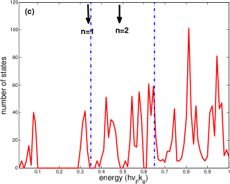
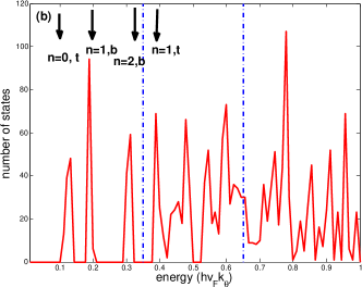
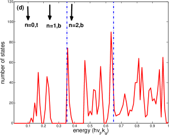
Figure 1: (Color online). The density of states of twisted bilayer graphene with $\theta=5^{\circ}$ and $w=0.15$ are shown. In (a) and (c) [(b) and (d)] the interlayer bias $u=0$ ($u=0.2$), and the magnetic field is $B=$ 28.5 (38.8) Tesla in (a) and (b) [(c) and (d)]. Arrows are used to indicate the first and second Landau levels in the case without interlayer coupling. The saddle point $E_{sp}=1/2-w$ and bottom of quadratic band $E_{bq}=1/2+w$ in the zero-field band structure are marked by the blue dashed lines.

The spectrum of twisted bilayer graphene is obtained by diagonalizing the matrix representation of the Hamiltonian in Eq. (1) in the basis $\{|n,m\rangle,n\geq 0,m\geq-n\}$, keeping only states consistent with a particular choice of $\nu$ in Eq. 9. For convenience we adopt $\hbar v_{F}k_{\theta}$ as our unit of energy. The magnetic field in tesla ($T$) is then given by

$$B=\frac{8.5\times 10^{4}}{(k_{\theta}\ell)^{2}}\theta^{2}[T]\>,$$ (11)

where the twist angle $\theta$, in units of radians in this equation, is assumed to be small. $\ell\equiv\sqrt{\hbar c/eB}$ is the magnetic length. For concreteness we consider a twisted bilayer graphene with $\theta=5^{\circ}$, which corresponds to $\hbar v_{F}k_{\theta}=665$ meV. We also consider a relatively strong field regime, in the sense that the dimensionless number $k_{\theta}\ell$ is of order one. By doing so, we need only a relatively small number of Landau levels to obtain results well-converged with respect to the maximum Landau level index retained in the calculation. In addition, we retain the same number of angular momentum states for each Landau level. The results we present are also well-converged with respect to this number.

Fig. 1 shows the density of states for the $\nu=0$ sector of the Hamiltonian in Eq. (1) for two magnetic fields, with and without interlayer bias. (Results for $\nu=1$ and $\nu=2$ are almost identical to this, so that distinguishing among the three sectors from their densities of states appears to be impractical.) The panels (a) and (b) are for $B=28.5T$, and in (c) and (d) $B=38.8T$; upper panels (a) and (c) are results without interlayer bias, while in the lower ones (c) and (d) $u=0.2$. The arrows indicate positions of Landau levels in the absence of interlayer tunneling, and for the lowest few Landau indices $n$ we can see that even with interlayer tunneling, density of states peaks can be assigned a definite Landau level index, although they are broadened relative to the case with no interlayer tunneling. This broadening becomes more pronounced with increasing $n$, and is especially pronounced when the unperturbed level approaches the saddle point energy $E_{sp}=1/2-w$ LuFertig14 . An example of this can be seen in Fig. 1(a), where the $n=2$ peak overlaps with $E_{sp}$ (shown as a dashed blue line in the figure.) One may also see the $n=1$ peak is broader in (c) than in (a), where in the former case it is closer to $E_{sp}$. Therefore, we may identify $E_{sp}$ as an energy scale separating regimes where the effects of interlayer tunneling are perturbative from one in which the density of states is qualitatively affected by interlayer tunneling. For energies above the quadratic band edge $E_{qb}=1/2+w$ LuFertig14 , and $u=0$, the density of states continues to oscillate but no longer actually vanishes, indicating that Landau level mixing has become important at this energy scale. Finally, we note also that the zeroth Landau level in our calculation is broadened and even split by the interlayer coupling. This effect appears to be particularly pronounced in strong fields, and can also be seen in tight-binding calculations Landgraf2013 .

The bottom two panels of Fig. 1 illustrate the effect of interlayer bias. One may see that the Landau level peaks below $E_{sp}$ are shifted by $\pm u$, but the features above this energy are less sensitive to bias, particularly in the range $E_{sp}<E<E_{qp}$. This is clearest in panel (b), where the minima in the spectrum above $E_{sp}$ move little in response to $u$, although the peak heights and widths show some sensitivity to bias. With the exception of the $n=2$ level associated with the bottom layer, this also seems to be the case in panel (d). Above $E_{qb}$, some minima are relatively unaffected by $u$, but some are, and at high enough energy the overall line shape changes significantly when $u$ is introduced [most noticeably in our results in panel (b)]

Figure 2: Evolution of semiclassical orbits in momentum space, near a saddle point. Panel (a) represents an orbit with energy below the saddle point with the upper (lower) part representing the trajectory in the top (bottom) layer. The tunnel coupling between these orbits is relatively weak and can be well-approximated as localized in a single layer. As the energy increases above $E_{sp}$, in the absence of interlayer coupling the two orbits cross (b). With tunneling there are two new orbits as illustrated in (c), and the closed orbit illustrated represents a branch of allowed states when the energy exceeds $E_{qb}$. The reconnected orbits now oscillate between layers, and the corresponding states are manifestly delocalized between them.

This mixed behavior may be understood in terms of the semiclassical description of wavefunctions in a magnetic field, which are built up from semiclassical orbits in the Brillouin zone, leading to some some wavefunctions being more strongly coupled across the layers than others. Fig. 2 illustrates one way in which this description leads to such a change in character. For states with energy well below $E_{sp}$, the semiclassical orbits LuFertig14 are weakly tunnel-coupled between layers across saddle points [Fig. 2(a)], with this coupling increasing greatly as the energy rises above $E_{sp}$ [Fig. 2(c)]. When tunneling can be ignored, wavefunctions can be associated with a particular layer, and their energies will shift by $\pm u$ when interlayer bias is introduced. When interlayer coupling is strong, one may consider the effect of $u$ within first order perturbation theory, and the energies of states that are equally distributed between the two layers will be unaffected by bias to this order. Thus, the sensitivity of the density of states to interlayer bias offers a measure of how strongly coupled the wavefunctions are between the two layers at a given energy.

We next turn to calculations of electromagnetic absorption (i.e., cyclotron resonance), which which we will see is directly impacted by the behaviors residing in the density of states.

IV Cyclotron resonance

In this section, we analyze electromagnetic absorption – i.e., cyclotron resonance – in this system, to see what one learns about the energy spectrum and also the extent to which wavefunctions are localized in one or the other layer. We will consider the absorption of linearly polarized waves, in which the polarization vector may be either parallel or perpendicular to the plane of the sample. Only the first of these induces transitions in single layer systems. In the bilayer system, the second can induce transitions between states if one or both of them is significantly delocalized between the layers. In this way cyclotron resonance can give us information about the nature of the wavefunctions.

IV.1 In-plane electric field

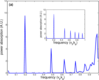
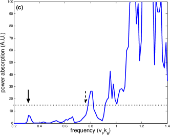
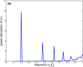
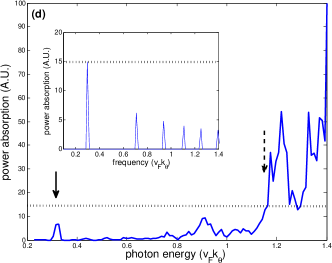
Figure 3: (Color online). Results of the cyclotron resonance for $\mu=0$ with the external electric field lying in plane. The magnetic field $B$ = 13 (28.5) Tesla in panel (a) and (b) [(c) and (d)]. The top panels (a) and (c) have zero interlayer bias while the bottom panel (c) [(d)] has the interlayer bias $u=$ 0.1 (0.2). The insets in (a) and (d) shows the corresponding results in the absence of interlayer coupling.

When the electric field of the perturbing radiation is in-plane, the resulting perturbation, with appropriate alignment with respect to the coordinate axes, is proportional to

$$\hat{x}=\frac{a+a^{{\dagger}}+b+b^{{\dagger}}}{\sqrt{2}}\>,$$ (12)

where the magnetic length $\ell$ has been set to one. The ladder operators in this expression acting on the basis states obey the relations

$$a^{{\dagger}}|n,m\rangle=\sqrt{n+1}|n+1,m-1\rangle\>,$$ (13)

$$\ b^{{\dagger}}|n,m\rangle=\sqrt{n+m+1}|n,m+1\rangle\>.$$ (14)

The operator $\hat{x}$ always changes the angular momentum by one, from which we can conclude that $\langle\Phi^{\nu}|\hat{x}|\Phi^{\nu}\rangle$ must vanish. Thus only transitions between sectors of different $\nu$ can contribute to cyclotron resonance in this configuration. From Fermi’s Golden Rule, for a given chemical potential $\mu$, the energy absorption $\alpha$ as a function of frequency $\omega$ becomes

$$\alpha(\omega)/\alpha_{0}=\omega\sum_{\hbar\omega_{f}>\mu}\sum_{\hbar\omega_{i}<\mu}|\langle f|\hat{x}|i\rangle|^{2}\delta(\omega_{f}-\omega_{i}-\omega)\>,$$ (15)

where $\alpha_{0}$ is an overall absorption scale, $|i(f)\rangle$ is the initial (final) single particle state, and $\hbar\omega_{i(f)}$ is the energy of that state. $\alpha(\omega)$ is essentially the real part of the dynamical conductivity Gusynin ; Moon3 , and our matrix diagonalization gives us access to both the wavefunctions and energies so we may compute it directly.

The results with chemical potential $\mu=0$ are illustrated in Fig. 3. For single graphene layer, the corresponding absorption peaks satisfy a selection rule $|n_{f}|=|n_{i}|\pm 1$ Jiang07 ; the resulting spectrum is illustrated in the insets of Fig. 3(a) and (d) for $B=$ 13 and 28.5 Tesla, respectively. If we label the frequency for the first peak associated with the transition $n=0\rightarrow n=1$ as $\omega_{01}$, then one can find the next three peaks at the frequencies of $(1+\sqrt{2})\omega_{01}$, $(\sqrt{2}+\sqrt{3})\omega_{01}$, and $(2+\sqrt{2})\omega_{01}$. In a twisted bilayer, at low enough excitation frequencies only eigenstates with $|E|<E_{sp}$ can be involved, and as discussed above these states to a good approximation may be treated as layer-polarized. Thus we expect to see the same absorption peaks as in single-layer graphene for sufficiently low frequency. This expectation is indeed the case in our calculations. In panel (a), it can be seen that $\omega_{01}\approx 0.2$ and the first four peaks in the single-layer case also appear at same frequencies in the tBLG. In panel (c) where the field is stronger, however, only the peak indicated by solid arrows, at $\omega_{01}\approx 0.3$ is found to coincide with its counterpart in single-layer case. This can be inferred from Fig. 1(a) where the Landau levels of $n\geq 2$ are significantly distorted by interlayer coupling, and we begin to see deviations from the higher order peaks in the single layer response. Those peaks representing the layer-polarized nature of states become broader with increasing field once the final states move close to the saddle point, and eventually merge into the high-frequency spectra.

It is interesting to note that in the presence of interlayer bias – for example, the spectrum with $u=0.2$ illustrated in Fig. 3(d) – this peak is essentially the same in position and oscillator strength as for $u=0$, further confirming the single-layer nature of Landau levels with $|E|<E_{sp}$. For lower field, such insensitivity to $u$ is even more obvious as shown in panel (b) in which $u$=0.1 and the spectrum does not deviate from that in panel (a) below $\omega\sim 0.9$.

At higher frequencies, $\alpha(\omega)$ deviates more dramatically from the single layer behavior. Absorption is increased significantly when high-energy, layer-delocalized states participate in transitions. We indicate a threshold energy for this change in behavior by dashed arrows in Fig. 3(c) and (d), which we define as the lowest frequency at which the absorption exceeds the largest peak in the single-layer case (see inset). Note that this threshold energy does depend on the interlayer bias, as illustrated in the figure. We attribute the sensitivity to $u$ to the layer delocalized nature of eigenstates for $|E|>E_{sp}$. It is interesting to notice that the overall scale of absorption is much higher than what is found in single layer electromagnetic absorption at these relatively low frequencies. Although $\alpha(\omega)$ obeys an oscillator strength sum rule Sabio , this is possible because the absorption in the continuum model continues to high frequency, with peak heights only falling off as $1/\omega$ at large frequency. A finite value for the sum rule is only obtained by imposing an energy cutoff in the spectrum. Evidently, the interlayer coupling transfers much of this high frequency oscillator strength for uncoupled layers to much lower frequency for tBLG. Clearly this is a non-perturbative effect.

Our general observation for this type of measurement is that at low frequency one expects to reproduce the single layer absorption spectrum, with strong deviations setting in once levels above $E_{sp}$ become involved. In principle, by examining the spectrum as a function of field and observing the frequency scale at which the deviation sets in, one may infer the value of $E_{sp}$ for the system. It is also possible to make this identification by looking for very low-energy, intra-Landau level absorption, which first becomes significant when a Landau level approximately coincides in energy with $E_{sp}$. We discuss this possibility in the next section.

IV.2 Out-of-plane electric field

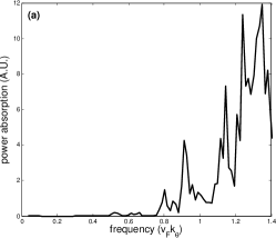
Figure 4: Results of the cyclotron resonance for $\mu=0$ with the external electric field parallel with the normal of plane. The magnetic field $B$ = 28.5 Tesla, and panel (a) and (b) are results without and with interlayer bias.

Next we consider the electric field polarized along the normal to the graphene plane. As remarked above, this can induce transitions because of the bilayer structure. In this case, the perturbation due to the vertical electric field is, up to an overall constant, the Pauli matrix $\tau_{z}$, acting on the two-dimensional layer space. This preserves the symmetry of the rotation operator $G$ in Eq. (6). Thus only the transitions within same sector $\nu$ are possible. The absorption as a function of frequency in this case can be written as

$$\alpha_{V}(E)/\alpha_{V}^{0}=\omega\sum_{\hbar\omega_{f}>\mu}\sum_{\hbar\omega_{i}<\mu}|\langle f|\tau_{z}|i\rangle|^{2}\delta(\omega_{f}-\omega_{i}-\omega)\>.$$ (16)

Fig. 4(a) and (b) show the results for the out-of-plane configuration with and without interlayer bias. In contrast with the in-plane configuration, it can be seen that the transition associated with single-layer behavior is completely absent, so that features relatively independent of interlayer bias $u$ are not present. The threshold frequency beyond which absorption increases markedly is sensitive to the interlayer bias, just as in the in-plane polarization case.

We may also use this configuration to explore the saddle point in the band structure. As mentioned above, the power absorption will vanish in the limit that the interlayer coupling $w\rightarrow 0$, so that absorption in this configuration is sensitive to whether the states are delocalized across the layers. One way in which this is manifested is the broadening of Landau levels as they cross the saddle point with increasing field. This admits the possibility of intra-Landau level absorption. Such absorption is highly suppressed in single layers because it can only occur when there is some perturbation that can relax the selection rule. In this case the perturbation is the interlayer coupling.

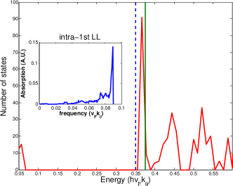
Figure 5: (Color online). Evolution of the density of states as the first Landau level passes through the saddle point (marked by the blue dashed line) with increasing field. In the right (left) panel, $B=$ 38.8 (46.6) Tesla. In the insets, the power absorption resulting from excitations within the first Landau level are shown. (Fermi levels are marked by green solid lines in the main panels.) A significant increase is seen as the first Landau level passes through the saddle point.

To carry this out one must be able to locate the Fermi level so that half the states of the broadened Landau level are filled, which in principle is possible via gating. One then adjusts the magnetic field so that the first Landau level passes through the saddle point (while keeping the level half filled.) Fig. 5 shows two density of states plots in which the $n=1$ Landau levels are pushed toward higher energy, broadening and and deforming the peak in the process. This broadening creates the possibility of electromagnetic absorption at very low-frequencies due to the intra-Landau level transitions. Shown in the insets are the absorption spectra, which now contain a low-energy peak. Comparing the two peaks for the Landau level just below and just above the saddle point, one can see a dramatic increase in both the maximum peak height and its oscillator strength as the Landau level center passes from just below to just above the saddle point energy. Fig. 6 shows results for the oscillator strength (obtained by numerically integrating the area under the peaks such as shown in the insets of Fig. 5) as a function of the “center” of the Landau level. This oscillator strength essentially starts to grow for $\mu$ just below $E_{sp}$, and has a sharp increase close to, although slightly below, the actual value of $E_{sp}$. In principle this provides a way to locate the energy of the saddle points separating the two Dirac points of the twisted bilayer.

V Conclusions

Figure 6: Integrated power absorption for the intra-Landau level transition. Horizontal axis: the chemical potential which is tuned to coincide with the center of first Landau level as the magnetic field varies. Vertical axis: the integrated power absorption due to the transition within the first Landau level. The two asymptotic lines intersect at an energy close to the saddle point.

We have studied the density of states and cyclotron resonance for Landau levels of tBLG within a continuum model. The model supports a three-fold symmetry which allows the states to be separated into three sectors, allowing some simplification of the numerical calculations. We find that the spectrum in a magnetic field evolves from discrete levels closely akin to single layer Landau levels into increasingly overlapping bands with increasing energy. Below the saddle point, the “band width” is very small and the magnetic states are mainly layer-polarized. Above the saddle point, the magnetic states becomes strongly layer-delocalized and the bands are significantly broader. This behavior follows from semiclassical descriptions of the wavefunctions, in which orbits in different layers begin to cross one another above the saddle point energy.

In order to explore the impact of interlayer coupling and related saddle points in the tBLG band structure, we propose two configurations for measuring electromagnetic absorption (cyclotron resonance) in this system. In one configuration the external electric field is polarized along the in-plane direction, and we find that as long as the magnetic field is not too strong, states below the saddle point are effectively layer-polarized and give rise to the same response as a single-layer system. On the other hand, the responses at higher frequencies involve layer-delocalized states. In the other configuration, where the electric field is polarized perpendicular to the system, layer delocalized states must be involved in the transitions. The different kinds of states may be distinguished by whether they can contribute to both types of absorptions, and by their sensitivity to interlayer bias.

We also found that the Landau level bands broaden significantly above the saddle point, so that power absorption becomes possible at very low frequency which is completely absent in the single layer case. In the perpendicular polarization configuration, we find the absorption increases significantly when the Landau band is elevated above the saddle point. In principle, this allows one to locate the saddle point energy from the absorption spectra of tBLG.

Acknowledgements This work was supported in part by the NSF through Grant No. DMR-1005035, and by the US-Israel Binational Science Foundation.

References

- (1) E. McCann and V. I. Falko, Phys. Rev. Lett. 96, 086805 (2006).
- (2) J. M. B. Lopes dos Santos, N. M. R. Peres, and A. H. Castro Neto, Phys. Rev. Lett. 99, 256802 (2007).
- (3) G. Li, A. Luican, J. M. B. Lopes dos Santos, A. H. Castro Neto, A. Reina, J. Kong, and E. Y. Andrei, Nat. Phys. 6, 109 (2010).
- (4) E V. Castro, K. S. Novoselov, S. V. Morozov, N. M. R. Peres, J. M. B. Lopes dos Santos, J. Nilsson, F. Guinea, A. K. Geim, and A. H. Castro Neto, Phys. Rev. Lett. 99, 216802 (2007).
- (5) I. Martin, Ya. M. Blanter, and A. F. Morpurgo, Phys. Rev. Lett. 100, 036804 (2008).
- (6) M. T. Allen, I. Martin, and A. Jacoby, Nat. Comm. 3, 934 (2012).
- (7) P. San-Jose and E. Prada, Phys. Rev. B 88, 121408 (2013).
- (8) C.-W. Huang, E. Shimshoni, H. A. Fertig, Phys. Rev. B 85, 205114 (2012).
- (9) V. Mazo, C.-W. Huang, E. Shimshoni, S. T. Carr, H. A. Fertig, Phys. Rev. B 89, 121411(R) (2014).
- (10) Z. Liu, K. Suenaga, P. J. F. Harris, and S. Iijima, Phys. Rev. Lett. 102, 015501 (2009).
- (11) A. L. Rakhmanov, A. V. Rozhkov, A. O. Sboychakov, and F. Nori , Phys. Rev. Lett. 109, 206801 (2012).
- (12) L. Brey and H. A. Fertig, Phys. Rev. B 87, 115411 (2013).
- (13) E. Suarez Morell, P. Vargas, L. Chico, and L. Brey, Phys. Rev. B 84, 195421 (2011).
- (14) D. S. Lee, C. Riedl, T. Beringer, A. H. Castro Neto, K. von Klitzing, U. Starke, and J. H. Smet, Phys. Rev. Lett. 107 216602 (2011).
- (15) K. Kim, S. Coh, L. Z. Tan, W. Regan, J. M. Yuk, E. Chatterjee, M. F. Crommie, M. L. Cohen, S. G. Louie, and A. Zettl, Phys. Rev. Lett. 108, 246103 (2012).
- (16) T. Ohta, J. T. Robinson, P. J. Feibelman, A. Bostwick, E. Rotenberg, and T. E. Beechem, Phys. Rev. Lett. 109, 186807 (2012).
- (17) L. Van Hove, Phys. Rev. 89, 1189 (1953).
- (18) J. Gonzalez, Phys. Rev. B 78, 205431 (2008).
- (19) R. Nandkishore, L. Levitov, and A. Chubukov, Nat. Phys. 8, 158 (2012).
- (20) J. Gonzalez, Phys. Rev. B 88, 125434 (2013).
- (21) For a review, see E. J. Mele, J. Phys. D: Appl. Phys. 45, 154004 (2012).
- (22) C.-K. Lu and H. A. Fertig, Phys. Rev. B 89, 085408 (2014).
- (23) T. Stauber, P. San-Jose, and L. Brey, New J. Phys. 15, 113050 (2013).
- (24) P. Moon and M. Koshino, Phys. Rev. B 87, 205404 (2013).
- (25) R. de Gail, M. O. Goerbig, F. Guinea, G. Montambaux, and A. H. Castro Neto, Phys. Rev. B 84, 045436 (2011).
- (26) M.-Y. Choi, Y.-H. Hyun, and Y. Kim, Phys. Rev. B 84, 195437 (2011).
- (27) D. Hofstadter, Phys. Rev. B 14, 2239 (1976).
- (28) P. Moon and M. Koshino, Phys. Rev. B 85, 195458 (2012).
- (29) L. A. Ponomarenko, R. V. Gorbachev, G. L. Yu, D. C. Elias, R. Jalil, A. A. Patel, A. Mishchenko, A. S. Mayorov, C. R. Woods, J. R. Wallbank, M. Mucha-Kruczynski, B. A. Piot, M. Potemski, I. V. Grigorieva, K. S. Novoselov, F. Guinea, V. I. Fal’ko and A. K. Geim Nature 497, 594 (2013).
- (30) C. R. Dean, L. Wang, P. Maher, C. Forsythe, F. Ghahari, Y. Gao, J. Katoch, M. Ishigami, P. Moon, M. Koshino, T. Taniguchi, K. Watanabe, K. L. Shepard, J. Jone, and P. Kim, Nature 497, 598 (2013).
- (31) R. Bistritzer and A. H. MacDonald, Phys. Rev. B 84, 035440 (2011).
- (32) Z. Jiang, E. A. Henriksen, L. C. Tung, Y.-J. Wang, M. E. Schwartz, M. Y. Han, P. Kim, and H. L. Stormer, Phys. Rev. Lett. 98 197403 (2007).
- (33) R. S. Deacon, K.-C. Chuang, R. J. Nicholas, K. S. Novoselov, and A. K. Geim, Phys. Rev. B 76 081406 (2007).
- (34) E. A. Henriksen, Z. Jiang, L. C. Tung, M. E. Schwartz, M. Takita, Y.-J. Wang, P. Kim, and H. L. Stormer, Phys. Rev. Lett. 100 087403 (2008).
- (35) M. Orlita, L. Z. Tan, M. Potemski, M. Sprinkle, C. Berger, W. A. de Heer, S. G. Louie, and G. Martinez, Phys. Rev. Lett. 108 247401 (2012).
- (36) Strictly speaking, any eigenstate of the system will be delocalized between both layers. However, in general one may form linear combinations of states that are localized in a single layer. If these are close in energy then the state can be usefully thought of as localized in a single layer. This turns out to be especially true for states at energies well below that of the saddle point. Sensitivity of the wavefunction energies to interlayer bias gives one measure of interlayer coupling inherent to the wavefunctions.
- (37) J. K. Jain, Composite Fermions, Cambridge University Press (2007).
- (38) W. Landgraf, S. Shallcross, K. Turschmann, D. Weckbecker, and O. Pankratov, Phys. Rev. B 87, 075433 (2013).
- (39) V. P. Gusynin and S. G. Sharapov, Phys. Rev. B 73, 245411 (2006)
- (40) P. Moon and M. Koshino, Phys. Rev. B 88, 241412 (2013).
- (41) J. Sabio, J. Nilsson, and A. H. Castro Neto, Phys. Rev. B 78, 075410 (2008).
- (42) J. M. Pereira, F. M. Peeters, and P. Vasilopoulos, Phys. Rev. B 76, 115419 (2007).