Interacting nonlinear wave envelopes and rogue wave formation in deep water

Abstract

A rogue wave formation mechanism is proposed within the framework of a coupled nonlinear Schrödinger (CNLS) system corresponding to the interaction of two waves propagating in oblique directions in deep water. A rogue condition is introduced that links the angle of interaction with the group velocities of these waves: different angles of interaction can result in a major enhancement of rogue events in both numbers and amplitude. For a range of interacting directions it is found that the CNLS system exhibits significantly more extreme wave amplitude events than its scalar counterpart. Furthermore, the rogue events of the coupled system are found to be well approximated by hyperbolic secant functions; they are vectorial soliton-type solutions of the CNLS system, typically not considered to be integrable. Overall, our results indicate that crossing states provide an important mechanism for the generation of rogue water wave events.

Even in the age of modern ship building and innovative navigation equipment, ship accidents are an important area of maritime concern. In recent years researchers have been investigating a topic which heretofore had been reserved for marine folklore: giant waves that seem to appear from nowhere in high seas that can lead to disastrous outcomes. These waves have, nowadays, been documented to exist and are usually referred to as rogue or freak waves.

The conditions that cause such waves to grow enormously in size are a topic of great interest with many different hypotheses being proposed Slunyaev, Kharif, and Pelinovsky (2009); Slunyaev, Didenkulova, and Pelinovsky (2011). An important one is the nonlinear mechanism of the self-wave interactions, such as modulation instability; in water wave physics this is called the Benjamin-Feir instability Benjamin and Feir (1967) and has been found under certain conditions to produce significant wave amplification.

The envelope of nonlinear water waves, under suitable conditions, is modeled by a nonlinear Schrödinger equation (NLS) Ablowitz (2011). Interestingly enough, the NLS not only gives a suitable description of these waves Dysthe, Krogstad, and Müller (2008); Müller, Garrett, and Osborne (2005); Slunyaev, Didenkulova, and Pelinovsky (2011); Chabchoub, Hoffmann, and Akhmediev (2011); Grimshaw et al. (2010); Shats, Punzmann, and Xia (2010), it is also an important equation used to investigate propagation of pulses in many other physical systems such as nonlinear optical fibers Hasegawa and Kodama (1995); Pisarchik et al. (2011); Bonatto et al. (2011); Zaviyalov et al. (2012), Bose-Einstein condensates Bludov, Konotop, and Akhmediev (2009), magnetic spin waves Patton et al. (1999) and many others.

The state of the sea in which rogue waves form is often complex Onorato, Osborne, and Serio (2006); Onorato et al. (2001); Ruban (2007) with certain key wave interactions dominating the wave structure. Here we focus on a coupled NLS (CNLS) system, derivable directly from the Euler equations. Underlying the wave phenomena are separate wave trains, propagating in different directions which interact at different angles; this provides a useful model of crossing sea states Adcock et al. (2011); Toffoli et al. (2011); Cavaleri et al. (2012); Laine Pearson (2010); Onorato, Osborne, and Serio (2006). The scalar NLS equation would be insufficient to describe these phenomena (rogue events associated with 2D scalar NLS equations are discussed in Ref. Buvoli (2013)).

As with the scalar problem the CNLS system exhibits modulation instability (MI), which as mentioned above, is an important aspect of rogue wave dynamics. Indeed, recent optical experiments indicate that MI is critical in the generation of strong optical rogue wave phenomena Solli et al. (2007). Previous studies have considered the growth rate of the underlying MI associated with CNLS equations Onorato, Osborne, and Serio (2006). It was found Kourakis and Shukla (2006); Onorato, Osborne, and Serio (2006) that the CNLS system can have significantly higher growth rates than the scalar NLS equation and thus MI will be triggered sooner. Here we find that for certain angles of wave interaction the CLNS system leads to large amplitude rogue waves and there can be more events than in the scalar NLS analogue. For other angles of interaction, we find another interesting result: while the growth rate can be higher in the CNLS system, it does not necessarily result in more significant events than its scalar counterpart.

Modulational instability and the wave angles of interaction of the waves in the CNLS system are directly linked to the coefficients of the system. The strongest rogue wave effect is found when both equations in the CNLS system are of focusing type. In fact, for special values of these coefficients the CNLS is integrable Manakov (1974). For the scalar NLS equation, when dispersion and nonlinearity share the same signs, the equation is said to be focusing, and the equation is modulationaly unstable; it is stable when the signs are opposite and the equation is said to be defocusing. The stability criteria are more involved for the coupled system Kourakis and Shukla (2006).

Here, we introduce the concept of a rogue condition which allows the two (spatial) dimensional water wave amplitude system to be reduced to a family of one dimensional CNLS systems. Indeed rogue events of associated one-dimensional equations such as the NLS equation has been a major topic of research in the study of rogue waves. It is found that there is a direct link between the rogue condition, i.e. the angle of interaction, and the number and magnitude of rogue events. We show that for certain angles this has a major effect on the associated wave events. Thus this rogue condition is not only related to the MI mechanism but also to the number and severity of events. A key aspect of this work is to investigate this rogue condition via direct calculation of probability distributions. We do not discuss the details of the underlying statistics which a separate topic and is outside the scope of this paper. For our purposes a basic probability density function distribution explains the salient points.

The nature of these rogue events is also an important issue addressed here. Rogue waves are commonly associated in the literature with rational-type solutions Peregrine (1983); Akhmediev, Eleonskii, and Kulagin (1987) of the scalar integrable NLS equation. We show that the rogue events associated with the CNLS equation are well approximated by hyperbolic secant functions. They propagate as solitary wave or soliton-type solutions of the CNLS system, which is not known to be integrable. Integrable equations exhibit rational solutions which are limits of multi-soliton solutions Ablowitz and Segur (1981) which by their very nature are associated with integrable systems like the scalar NLS equation.

Since we will be analyzing coupled NLS equations that arise in water waves it is convenient to review the analysis beginning with the Euler equations appropriate for describing waves in deep water

$$\nabla^{2}\phi=0,\quad-\infty<z<\varepsilon\eta$$

$$\phi_{z}=0,\quad z\rightarrow-\infty$$

$$\eta_{t}+\varepsilon(\eta_{x}\phi_{x}+\eta_{y}\phi_{y})=\phi_{z},\quad z=\varepsilon\eta$$

$$\phi_{t}+g\eta+\frac{\varepsilon}{2}(\phi_{x}^{2}+\phi_{y}^{2}+\phi_{z}^{2})=0,\quad z=\varepsilon\eta$$

where $\phi$ is the velocity potential, $\eta$ the surface elevation, $g$ gravity, $\bm{\nabla}=(\partial/\partial x,\partial/\partial y)$ and $\varepsilon$ is a small parameter. Define the multiple scales $X=\varepsilon x$, $Y=\varepsilon y$, $Z=\varepsilon z$, $T=\varepsilon t$, expand $\phi=\phi(t,x,y,\varepsilon\eta)$ around $z=0$, and all fields in powers of $\varepsilon$ as follows

$$\phi=\phi_{0}+\varepsilon\phi_{1}+\mathcal{O}(\varepsilon^{2})$$

$$\eta=\eta_{0}+\varepsilon\eta_{1}+\mathcal{O}(\varepsilon^{2}).$$

At leading order, $\mathcal{O}(1)$, we assume two wave trains

$$\phi_{0} =A(X,Y,Z,T)e^{i\theta_{1}+\Omega_{1}z}+B(X,Y,Z,T)e^{i\theta_{2}+\Omega_{2}z}+\mathrm{cc}$$ (1a)

$$\eta_{0} =N(X,Y,T)e^{i\theta_{1}}+M(X,Y,T)e^{i\theta_{2}}+\mathrm{cc}$$ (1b)

where $\theta_{i}=k_{i}x+l_{i}y-\omega_{i}t$, $(i=1,2)$, $\Omega_{i}=\sqrt{k_{i}^{2}+l_{i}^{2}}$, $\omega_{i}^{2}=g\sqrt{k_{i}^{2}+l_{i}^{2}}$ and cc denotes complex conjugate. Using the above and removing secular terms the following set of coupled equations is obtained

$$i\left({\frac{{\partial{A}}}{{\partial{T}}}+{{\mathbf{v}}_{1}}\cdot\bm{\nabla}{A}}\right)+\varepsilon\left(\frac{1}{2}\frac{{{\partial^{2}}{\omega_{1}}}}{{\partial k_{1}^{2}}}\frac{{{\partial^{2}}{A}}}{{\partial X^{2}}}+\frac{{{\partial^{2}}{\omega_{1}}}}{{\partial{k_{1}}\partial{l_{1}}}}\frac{{{\partial^{2}}{A}}}{{\partial{X}\partial{Y}}}\right.$$

$$+\left.\frac{1}{2}\frac{{{\partial^{2}}{\omega_{1}}}}{{\partial l_{1}^{2}}}\frac{{{\partial^{2}}{A}}}{{\partial Y^{2}}}+({q_{11}}|{A}{|^{2}}+{q_{12}}|{B}{|^{2}}){A}\right)=0\hfill$$ (2a)

$$i\left({\frac{{\partial{B}}}{{\partial{T}}}+{{\mathbf{v}}_{2}}\cdot\bm{\nabla}{B}}\right)+\varepsilon\left(\frac{1}{2}\frac{{{\partial^{2}}{\omega_{2}}}}{{\partial k_{2}^{2}}}\frac{{{\partial^{2}}{B}}}{{\partial X^{2}}}+\frac{{{\partial^{2}}{\omega_{2}}}}{{\partial{k_{2}}\partial{l_{2}}}}\frac{{{\partial^{2}}{B}}}{{\partial{X}\partial{Y}}}\right.$$

$$+\left.\frac{1}{2}\frac{{{\partial^{2}}{\omega_{2}}}}{{\partial l_{2}^{2}}}\frac{{{\partial^{2}}{B}}}{{\partial Y^{2}}}+({q_{21}}|{A}{|^{2}}+{q_{22}}|{B}{|^{2}}){B}\right)=0\hfill$$ (2b)

where $\mathbf{v}_{i}=(\partial\omega_{i}/\partial k_{i},\partial\omega_{i}/\partial k_{i})^{\mathrm{T}}$ and

$$q_{11}=-\frac{2\omega_{1}^{7}}{g^{4}},\quad q_{22}=-\frac{2\omega_{2}^{7}}{g^{4}}$$

$$q_{12}=-\frac{1}{\omega_{1}}\left[m_{12}^{2}+\frac{4m_{12}}{g^{2}}\omega_{1}\omega_{2}^{3}-\frac{\omega_{1}^{4}\omega_{2}^{4}}{g^{4}}\right]$$

$$q_{21}=-\frac{1}{\omega_{2}}\left[m_{12}^{2}+\frac{4m_{12}}{g^{2}}\omega_{1}^{3}\omega_{2}-\frac{\omega_{1}^{4}\omega_{2}^{4}}{g^{4}}\right]$$

where $m_{12}=k_{1}k_{2}+l_{1}l_{2}$. These coefficients are in agreement with the ones found in Refs. Benney (1962); Roskes (1976a); Hammack, Henderson, and Segur (2005). Indeed, the nonlinear coefficients all agree because they do not depend on derivatives of the fields $A$, $B$. Similarly, the coefficients of the linear terms are associated with the underlying linear dispersion relation of water waves; this is universal for NLS systems.

The relationship between the velocity potential $\phi$ and the wave elevation $\eta$ is obtained via

$$N=\frac{i\omega_{1}}{g}A,\quad M=\frac{i\omega_{2}}{g}B.$$

Next introduce new projection coordinates such that

$$\xi_{1}=\cos\theta X+\sin\theta Y-\left(\cos\theta\frac{\partial\omega_{1}}{\partial k_{1}}+\sin\theta\frac{\partial\omega_{1}}{\partial l_{1}}\right)T$$

$$\xi_{2}=\cos\theta X+\sin\theta Y-\left(\cos\theta\frac{\partial\omega_{2}}{\partial k_{2}}+\sin\theta\frac{\partial\omega_{2}}{\partial l_{2}}\right)T$$

and demand that we have only one projected coordinate, $\xi_{1}=\xi_{2}=\xi$, i.e.

$$\cos\theta\frac{\partial\omega_{1}}{\partial k_{1}}+\sin\theta\frac{\partial\omega_{1}}{\partial l_{1}}=\cos\theta\frac{\partial\omega_{2}}{\partial k_{2}}+\sin\theta\frac{\partial\omega_{2}}{\partial l_{2}}\Leftrightarrow$$

$$\tan\theta=-\frac{\partial\omega_{1}/\partial k_{1}-\partial\omega_{2}/\partial k_{2}}{\partial\omega_{1}/\partial l_{1}-\partial\omega_{2}/\partial l_{2}}$$ (3)

We refer to Eq. (3), which links the angle of interaction with the wave numbers of the relative waves, as the rogue condition. Note, that if more than two wave packets are present this condition is much more restrictive as the resulting system of equations will be satisfied only for certain wave numbers Roskes (1976b). It is important to observe that transforming to projection coordinates, with the above rogue condition added, has the effect of matching the group velocities of the different cross wave states. If the group velocities were not matched then two localized states would evolve through one another and lead to minimal interaction. The rogue condition thus allows enhanced interaction.

This condition leads to a family of one dimensional coupled NLS systems all of which have the potential to generate rogue waves. This is more general than the case studied in Ref. Onorato, Proment, and Toffoli (2010) where wave numbers were chosen such that $k_{1}=k_{2}$ and $l_{1}=-l_{2}$. As such only one case whose projection moves along one preferred axis was considered. Furthermore, only the growth rates of modulation instability were considered and no comparisons between the NLS and the number and frequency of coupled systems’s rogue event statistics were made. Demonstrating statistically that more frequent and more serious rogue events occur in the coupled system shows that surely these systems must be considered as potential rogue event generators. We also note that our envelope equations are different from the those of Ref. Onorato, Osborne, and Serio (2006) which are derived from an approximation to the Euler equations. The equations here are derived directly from the Euler equations.

Moreover, the nonlinear Schrödinger equation (in 1+1: one space, one time dimension or even 2+1 dimensions) corresponds to wave packets –envelopes associated with a periodic wave train which is slowly varying in space. In the 1+1 NLS equation one considers only a one dimensional model along the direction of a wave train. In 2+1 one requires slow variation in both the direction of wave train and perpendicular to the wave train; in essence since the envelope is slowly varying, the 2+1 model itself can be considered as essentially quasi-one dimensional.

In general one can ask whether a sea state can be one dimensional. Indeed nearly one dimensional sea states are special situation but nearly one dimensional states can occur, and while these are somewhat unusual or special situations nevertheless the issue under study here is, by its very nature, special: i.e. a rogue event. One can also consider slowly varying waves both along and orthogonal to the direction to the wave train Buvoli (2013). As indicated above, without the one dimensional or nearly one dimensional reduction one expects that any localized disturbance in coupled NLS equations would pass through one another and there would be a relatively small resulting interaction.

Finally, with $\tau=\varepsilon T$ Eqs. (2) become

$$i\frac{{\partial{A}}}{{\partial\tau}}+{P_{1}}\frac{{{\partial^{2}}{A}}}{{\partial{\xi^{2}}}}+({q_{11}}|{A}{|^{2}}+{q_{12}}|{B}{|^{2}}){A}=0\hfill$$ (4a)

$$i\frac{{\partial{B}}}{{\partial\tau}}+{P_{2}}\frac{{{\partial^{2}}{B}}}{{\partial{\xi^{2}}}}+({q_{21}}|{A}{|^{2}}+{q_{22}}|{B}{|^{2}}){B}=0$$ (4b)

where $\displaystyle P_{i}=\frac{1}{2}\left[{{{\cos}^{2}}\theta\frac{{{\partial^{2}}{\omega_{i}}}}{{\partial k_{i}^{2}}}+\sin(2\theta)\frac{{{\partial^{2}}{\omega_{i}}}}{{\partial{k_{i}}\partial{l_{i}}}}+{{\sin}^{2}}\theta\frac{{{\partial^{2}}{\omega_{i}}}}{{\partial l_{i}^{2}}}}\right]$. Notably, Eqs. (4) have the same structure in dimensionless form. Indeed, introduce the nondimensional scaling: $k_{j}=k_{*}k^{\prime}_{j}$, $l_{j}=k_{*}l^{\prime}_{j}$, $j=1,2$ and $\tau^{\prime}=\omega_{*}\tau$, $\xi^{\prime}=k_{*}\xi$, $A^{\prime}=N_{*}A$, $B^{\prime}=N_{*}B$, where $N_{*}=g/(\omega_{*}/k_{*})$, $\omega_{*}^{2}=gk_{*}$ where $k_{*}$ is a typical wavelength in the ocean. The result, after dropping primes, is exactly the system of equations Eqs. (4) above.

As a prototypical situation in what follows we fix $k_{1}=k_{2}=1$ and $l_{1}=0$ and vary the angle $\theta$ so that $l_{2}$ is retrieved from Eq. (3). Furthermore, for convenience, introduce the change of variables:

$$\tau=\tau_{0}\tau^{\prime},\;\xi=\xi_{0}\xi^{\prime},\;A=A_{0}A^{\prime},\;B=B_{0}B^{\prime}$$

where, $\tau_{0}=-2\omega_{1}$, $\xi_{0}=\omega_{1}/(2k_{1})$ and $A_{0}=B_{0}=1/(2k_{1}^{2})$. Then after dropping primes, we obtain the system

$$iA_{\tau}+d_{1}A_{\xi\xi}+(g_{11}|A|^{2}+g_{12}|B|^{2})A =0$$ (5a)

$$iB_{\tau}+d_{2}B_{\xi\xi}+\left(g_{21}|A|^{2}+g_{22}|B|^{2}\right)B =0$$ (5b)

With the above values the coefficients of the system (5) vary with $\theta$ as shown in Fig. 1.

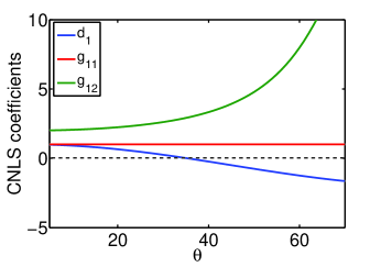
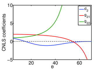
Figure 1: (Color online) The CNLS coefficients vs. the angle $\theta$.

We note that at about $\theta=35^{\circ}$ the zero dispersion limit of Eq. (5a) occurs ($d_{1}=0$) and similarly for Eq. (5b) at about $\theta=15^{\circ}$ and $65^{\circ}$ ($d_{2}=0$); here the above rescaling fails and a different scaling must be used. Finally note that as $\theta\rightarrow 90^{\circ}$ $|g_{21}|\rightarrow\infty$ and the equations uncouple with $A\rightarrow 0$.

The sign changes of the coefficients indicated in Fig. 1 also lead to changes in the modulational stability properties for Eqs. (5); this is summarized in Fig. 2. It is important to stress that growth rates and occurrence of rogue events and are not necessarily indicative of the wave statistics. Indeed, based on the results of Ref. Kourakis and Shukla (2006) the coupled system exhibits MI much faster than its scalar counterpart, i.e. has higher growth rates. This, however, may not result in more extreme events as will be shown here.

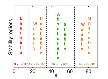
Figure 2: (Color online) The three stability regions of Eqs. (5).

We name these regions unstable (where both equations are focusing), weakly unstable (where one of the equations is focusing and the other defocusing) and absolutely stable (where both equations are defocusing). Recall Kourakis and Shukla (2006), that the stability criteria are different for the scalar and coupled NLS systems. However, if both equations are defocusing the CNLS is always stable.

We now integrate numerically Eqs. (5) using pseudospectral methods in space and exponential Runge-Kutta for the evolution Ref. Kassam and Trefethen (2005) in a computational domain $\xi\in[-100,100]$, $\tau\in[0,10]$. As a convenient and “typical” initial condition we choose a wide gaussian

$$A(\xi,0)=B(\xi,0)=e^{-\xi^{2}/2\sigma^{2}},\;\sigma=30$$

perturbed with 10% random noise for $10^{5}$ trials. A wide gaussian with randomness added is a prototype of a set of broad/randomly generated states. The Gaussian initial data we chose also has narrow band spectrum since we are looking at slowly varying waves around two cross wave. We can modify the distribution to look more like JONSWAP spectrum data (see below), but the essential purpose here, as indicated above is to show that the coupled system can lead to serious rogue events similar to, but more serious than the scalar NLS equation.

In each trial we measure the highest wave amplitude and introduce the quantity $\eta_{\mathrm{rel}}$ which is the ratio of the highest wave amplitude (as defined by Eq. (1b)) to the maximum of the initial condition. In the following figures we show the resulting probability density functions (PDF) for the two different regions of instability (in the stable region we see rogue events in neither the CLNS system nor the scalar defocusing NLS equation). It is found that the PDFs exhibit Rayleigh-like distributions (see Fig. 3) in line with our evaluation of the magnitude of the wave elevation. We do not go into the details of the differences between our distribution and Rayleigh distributions as such differences are not an essential aspect of this study.

We begin with the unstable region, Fig. 3.

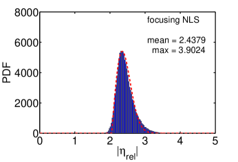
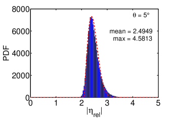
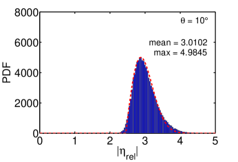
Figure 3: (Color online) The PDFs for the scalar focusing NLS (top) and unstable CNLS. A Rayleigh distribution with the same peak and scale factor as our calculated PDF is fitted (in red) on each PDF.

Here, both equations are focusing. It is clear that as the angle increases there is a significant shift in the mean of the PDF; the stronger the coupling the more events are produced in both number and magnitude. Thus we see that oblique interactions can lead to serious rogue events. In fact, for the focusing scalar case (which is obtained at $\theta=0$ with $B=0$) the number of rogue events (events of magnitude greater than three times the magnitude of the initial condition) is nearly 3% (2728/100000 events). Whereas for the coupled case of $\theta=10^{\circ}$ this percentage is above 22% (22317/100000 events).

We also demonstrate that both components play a role for large events; in Fig. 4 a typical rogue event is obtained from Eqs. (5) and the relative components that form it. Namely, in the top two figs we obtain $A$, $B$ and plot $A_{\mathrm{rel}}$, $B_{\mathrm{rel}}$ (i.e. $A$, $B$ divided by their respective initial conditions). Similarly from $A$, $B$ we obtain $M$, $N$ and find the wave elevation $\eta$ and plot $\eta_{\mathrm{rel}}$.

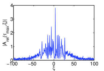
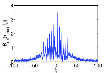
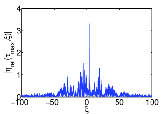
Figure 4: (Color online) A typical rogue event obtained from Eqs. (5). The time $\tau_{\mathrm{max}}$ indicates when the maximum (in amplitude) of this event occurs.

For completeness typical JONSWAP type initial data are also considered Onorato et al. (2013). No qualitative differences are found as shown in Fig. 5; namely the coupled system leads to far more rogue events than scalar NLS equation with these initial conditions. We use the values of the JONSWAP data from Ref. Onorato et al. (2013) along with Eq. (1b) with $M=N$ at $t=0$ to get the initial conditions for Eqs. (5).

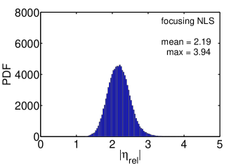
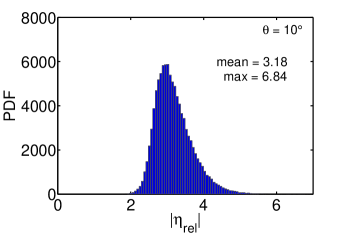
Figure 5: (Color online) The PDFs for the scalar focusing NLS (top) and unstable CNLS using JONSWAP data as initial conditions.

In the scalar NLS equation various modal shapes have been proposed as modes which describe rogue events, e.g. the Peregrine soliton Peregrine (1983); Akhmediev, Soto-Crespo, and Ankiewicz (2009); Chabchoub, Hoffmann, and Akhmediev (2011). The CNLS system described here, unlike cases which have different coefficients such as those considered in other studies Baronio et al. (2012), is not known to be integrable.

Below, we briefly examine the nature of the extreme rogue waves. While in the study of rogue phenomena the focus is the surface elevation $\eta$, the fundamental nature of the solutions of the system (5) shifts attention to the envelopes $A$ and $B$. Consider a typical extreme rogue event much like the one from Fig. 4. In order to investigate its properties we zoom in around the maximum height, see Fig. 6.

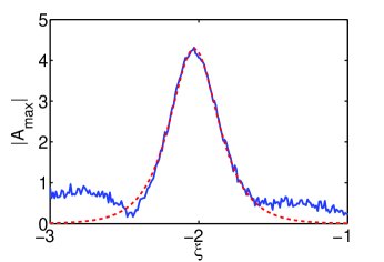
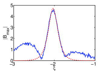
Figure 6: (Color online) A typical zoom-in on a rogue event and the relative fit from a hyperbolic secant.

Then the amplitude of the $A,B$ rogue wave is fitted with hyperbolic secant secant functions; we found that this anzatz gives a very good fit. It should be noted that these two profiles are not equal (as also seen from the figure) and are approximated as

$$\ A(\xi)=4.284\;\mathrm{sech}(6.852\xi),\;\;B(\xi)=\;4.724\;\mathrm{sech}(9.728\xi)$$

Next we evolve we use these profiles as, initial conditions for the CNLS system, Eqs. (5); we depict the evolution in Fig. 7.

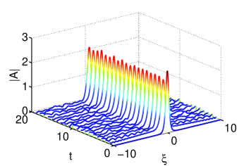
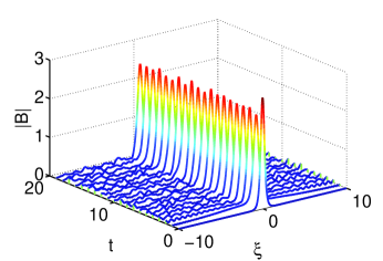
Figure 7: (Color online) The evolution of the envelope components of a rogue wave.

Remarkably, the initial condition holds its shape and position and propagates as an approximate solitary wave –soliton solution of the system. The small amount of radiation shed is to be expected as this is only an approximate solution to the system. However, it also attests to its stability as it does not break down or disperse as one may expect from a function which is not near a true solution. This sheds new light into the properties of rogue waves as they evidently can be solutions of what is not known/expected to be an integrable system. Similar results are obtained for other rogue events. Further comparisons and more detailed analysis will be carried out in a future communication.

We continue with the weak unstable region, Fig. 8. In this region one of the equations is focusing while the other is defocusing. Note here that for the CNLS system one still has unstable MI growth from the initial condition. However, in this case it produces fewer rogue events than that of the single scalar NLS equation–compare with Fig. 3 (top). As mentioned in the introduction it is important to note that despite the fact for this choice of parameters, the growth rate is greater in the CNLS system than that of the corresponding scalar NLS equation Kourakis and Shukla (2006) there are fewer not more rogue events generated in the coupled NLS system.

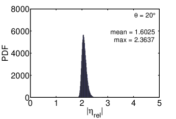
Figure 8: (Color online) The PDFs for the weakly unstable CNLS.

From the above analysis it is clear that the CNLS system not only corresponds to an interesting and physically relevant situation in deep water but it also produces novel and significantly different rogue phenomena than its scalar NLS counterpart. It is important to note that in certain parameter regimes a major increase in the number of rogue events can be produced from the CNLS system as compared with the scalar NLS equation. While rogue events are closely associated with MI, nevertheless larger MI growth rates do not always lead to more rogue events. Furthermore, these events are approximate solitary wave–soliton solutions of the coupled NLS system which is not known to be integrable. It appears unlikely that these solitary–soliton waves can be rational solutions since the latter are typically limits of multi-soliton solutions which are intimately related to integrable equations Ablowitz and Segur (1981).

To summarize, an interacting coupled NLS wave envelope system associated with the Euler equations in deep water with different group velocities is studied. In general, this system of equations exhibits modest nonlinear interaction since the group velocity terms would lead to the separation of localized states. However this coupled system can be reduced to the CNLS system by adding an additional restriction. This links the angle of interaction with the group velocities of the interacting waves. With this additional condition, referred to here as the rogue condition, it is found that depending on the angle of interaction, the coupled system can substantially enhance the number and size of rogue events as compared to the scalar NLS equation which itself has been linked to rogue wave phenomena. The type of rogue wave obtained from the CNLS system is vectorial in nature and as such is fundamentally different from the rogue events in the scalar NLS equation.