Parallel kinetic Monte Carlo simulation of Coulomb glasses

Abstract

We develop a parallel rejection algorithm to tackle the problem of low acceptance in Monte Carlo methods, and apply it to the simulation of the hopping conduction in Coulomb glasses using Graphics Processing Units, for which we also parallelize the update of local energies. In two dimensions, our parallel code achieves speedups of up to two orders of magnitude in computing time over an equivalent serial code. We find numerical evidence of a scaling relation for the relaxation of the conductivity at different temperatures.

1 Introduction

A frequent limitation of Markov-chain Monte Carlo (MC) methods is low acceptance. In equilibrium MC this problem can sometimes be circumvented with a clever choice of the MC moves, which can be chosen with a certain freedom as long as the Markov chain converges to the probability distribution of interest. Such freedom is not allowed in kinetic Monte Carlo (KMC), in which the MC moves are dictated by the physical dynamics to be simulated.

In this work we present a general “parallel rejection” (PR) algorithm to address the problem of low acceptance, which is especially suitable for implementation on Graphics Processing Units (GPUs), easily available and inexpensive platforms for massively parallel computing. We apply PR to the KMC simulation of the hopping conduction in Coulomb glasses, which is notoriously plagued by very low acceptance in the variable-range hopping (VRH) regime. For this particular application, PR can be seen as a parallelization of the “mixed” algorithm of Refs. Tsigankov and Efros (2002); Tsigankov et al. (2003), which can be further accelerated in GPUs by efficiently parallelizing the $N$ local energy updates that, due to the long-range interaction, are required after each elementary MC move in a system with $N$ sites.

We implemented a GPU code using CUDA CUD (2013), exploiting both sources of parallelism. In the next section we illustrate the PR idea in general, and later we apply it to the hopping dynamics of the Coulomb glass. We then present our results for the lattice model in two dimensions, notably on the short-time relaxation of the conductivity. Finally, we compare the performance of the GPU code with a serial implementation of the mixed algorithm.

2 Parallel rejection algorithm

Let us consider a generic Markov chain specified by a proposal matrix $Q_{\alpha\beta}$ and an acceptance matrix $P_{\alpha\beta}$ between the configurations $\alpha,\beta$ of a certain system. The standard (serial) rejection algorithm to simulate such a chain consists in iterating the following two steps: 1. Propose a move $\alpha\to\beta$, where $\alpha$ is the current configuration and $\beta$ is chosen with probability $Q_{\alpha\beta}$; 2. Accept the move with probability $P_{\alpha\beta}$ and, if this is accepted, update the configuration to $\beta$.

The PR algorithm (see Ref.Niemi and Wheeler (2011) for a similar idea) runs simultaneously on an ordered array of $M$ parallel “threads” (for example, GPU threads), iterating the following steps ($k=1,\dots,M$ is the thread label):

• Propose, independently from the other threads, a move $\alpha\to\beta_{k}$, where $\alpha$ is the current configuration (common to all threads) and $\beta_{k}$ is chosen with probability $Q_{\alpha\beta_{k}}$.

• Accept the move $\alpha\to\beta_{k}$ with probability $P_{\alpha\beta_{k}}$, independently from the other threads (without updating the configuration).

• If at least one thread has accepted a move, update the configuration to $\beta_{q}$, where $q$ is the lowest label among the threads that have accepted a move.

While the two algorithms above are mathematically equivalent (see Fig.1(a) for an illustration), the parallel version is increasingly faster as the acceptance rate, $A=\langle P_{\alpha\beta}\rangle$, decreases. If $m$ and $p$ are the number of iterations of the serial and parallel algorithms, respectively, until a move is accepted, we can estimate the speedup of PR as $\langle m\rangle/\langle p\rangle$ (neglecting parallelization overheads and differences in the computing time for one iteration in the parallel and serial implementations). Since $\langle m\rangle=A^{-1}$ and $\langle p\rangle=1/[1-(1-A)^{M}]$, for $A\ll 1$ we have $\langle p\rangle\sim(MA)^{-1}\ll\langle m\rangle$, and thus $\langle m\rangle/\langle p\rangle\sim{\mbox{min}}(A^{-1},M)$. In principle, the optimal choice for $M$ is thus $M^{*}={\mbox{min}}(A^{-1},C)$, where $C$ is the maximum number of threads that can run simultaneously. In practice, in a GPU implementation it is possible (and recommended) to use $M$ larger than $C$, in which case the virtual parallel execution is efficiently handled by the hardware scheduling system. The computing time can then remain sublinear in $M$ even for $M$ as large as $10^{4}$. Thus, for many applications the speedup of the PR algorithm on GPUs is essentially dictated by $~{}A^{-1}$, and can be very significant.

A popular alternative to the rejection algorithm in low-acceptance situations is the rejection-free BKL or Gillespie algorithm Bortz et al. (1975). This requires a computing time proportional to the average number $z=\langle\sum_{\beta}\theta(Q_{\alpha\beta}P_{\alpha\beta})\rangle$ of configurations that are accessible from a given configuration $\alpha$. Thus, BKL is faster than serial rejection when $z\ll A^{-1}$, but slower than PR when $(MA)^{-1}\ll z$. Below we apply PR to the rejection part of the mixed algorithm of Ref. Tsigankov and Efros (2002), which combines the BKL and rejection algorithms for the simulation of phonon-assisted hopping conduction.

3 Hopping conduction in the Coulomb glass

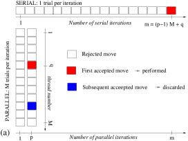
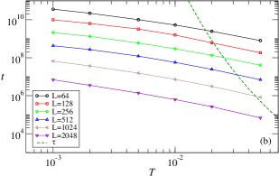
Figure 1: (a) Illustrative comparison of the “Parallel Rejection” scheme with the mathematically equivalent serial approach. In both, proposed moves (squares) are drawn by sampling from the proposal probability. While in the serial approach (top) one move is proposed each iteration, in the parallel approach (bottom) a block of $M$ independent moves is proposed. For a given acceptance rate, the first accepted move (red square) is found after $m$ serial iterations, and after $p$ parallel iterations. Other accepted moves (blue square) that may appear in last parallel iteration are discarded. In this example $M=12$, $p=2$, $q=5$. (b) Physical time (in units of $\tau_{0}$) that we can simulate with the parallel KMC method in a 10 days run, as a function of temperature, for different systems sizes. The dashed line is the characteristic time $\tau=b^{-1}T^{-1}\exp[(T_{0}/T)^{1/2}]$, with $b^{-1}=2.7,T_{0}=6.2$ according to Fig.3.

We consider the standard Coulomb glass model Efros (1976) described by the dimensionless Hamiltonian

$$H=\sum\phi_{i}n_{i}+\frac{1}{2}\sum_{i\neq j}\frac{(n_{i}-\nu)(n_{j}-\nu)}{r_{ij}}-E\sum_{i}n_{i}x_{i},$$ (1)

where $n_{i}=0,1$ ($i=1,\dots,N)$, with $\sum_{i}n_{i}=\nu N$, are the electron occupation numbers of $N$ sites in a $D$-dimensional volume, $\nu$ is the filling factor, $r_{ij}$ is the Euclidean distance between sites $i$ and $j$ in units of the average spacing $a=({\mbox{Volume}}/N)^{1/D}$, and $E$ is an external electric field in the (negative) $x$ direction. The random potentials $\phi_{i}$ are sampled from the uniform distribution $[-W,W]$. We consider only phonon-assisted single-electron hops, with transition rates that can be approximated by

$$\Gamma_{ij}=\tau_{0}^{-1}\theta_{ij}e^{-2r_{ij}/\xi}\min[1,e^{-\Delta H_{ij}/k_{B}T}]$$ (2)

where $T$ is the temperature, $k_{B}$ is the Boltzmann constant, $\theta_{ij}=\delta_{n_{i},1}\delta_{n_{j},0}$, $\xi$ is the electron localization length, and $\tau_{0}$ is a microscopic time of order $10^{-12}$s, which will be our unit of time. The energy change after a hop $i\to j$ is $\Delta H_{ij}=\epsilon_{j}-\epsilon_{i}-1/{r_{ij}}-E\Delta x_{ij},$ where $\epsilon_{i}=\phi_{i}+\sum_{j}(n_{j}-\nu)/r_{ij}$ are the single-particle energies and $\Delta x_{ij}=x_{j}-x_{i}$ is the length of the hop along the field. The instantaneous conductivity is given by Tsigankov and Efros (2002); Tsigankov et al. (2003)

$$\sigma(t)=\frac{1}{NE}\frac{dP(t)}{dt}$$ (3)

where $P=\sum_{i}n_{i}x_{i}$ is the electric dipole moment, provided $E$ is small enough to ensure a linear response.

In the naive serial KMC algorithm for simulating the dynamics in Eq.(2) a hop $i\to j$ is proposed by choosing $i$ and $j$ uniformly at random among the $N$ sites, and is accepted with probability $\tau_{0}\Gamma_{ij}$ (thus, $Q_{\alpha\beta}=N^{-1}(N-1)^{-1}\sum_{ij}\Theta^{ij}_{\alpha\beta}$ and $P_{\alpha\beta}=\sum_{ij}\tau_{0}\Theta^{ij}_{\alpha\beta}\Gamma_{ij}$, where $\Theta^{ij}_{\alpha\beta}=1$ if $\alpha$ and $\beta$ differ by the hop $i\to j$ and $\Theta^{ij}_{\alpha\beta}=0$ otherwise). The time is incremented by $\Delta t=1$ after $N(N-1)$ proposals.

The above algorithm suffers from extremely low acceptance due to both the tunneling factor $\Gamma_{ij}^{T}=e^{-2r_{ij}/\xi}$ and the thermal activation factor $\Gamma_{ij}^{A}=\theta_{ij}\min[1,\exp(-\Delta H_{ij}/T)]$. The mixed algorithm Tsigankov et al. (2003) exploits the factorization $\tau_{0}\Gamma_{ij}=\Gamma^{T}_{ij}\Gamma^{A}_{ij}$ and the fact that $\Gamma^{T}_{ij}$ is configuration independent. The proposal matrix is now $Q_{\alpha\beta}=\sum_{ij}\Theta^{ij}_{\alpha\beta}\Gamma^{T}_{ij}/\Gamma$, where $\Gamma=\sum_{i}\sum_{j\neq i}\Gamma^{T}_{ij}$, and can be sampled without rejection (for example, using the “tower sampling” method  Krauth (2006)). The acceptance matrix is $P_{\alpha\beta}=\sum_{ij}\Theta^{ij}_{\alpha\beta}\Gamma^{A}_{ij}$. After each proposal, $t$ is incremented by a random $\Delta t$ sampled from $p(\Delta t)=\Gamma\exp(-\Gamma\Delta t)$ Bortz et al. (1975). Since the rejection now only comes from $\Gamma^{A}_{ij}$, the acceptance rate is increased by a factor $\sim N\xi^{-D}$. Nevertheless, deep in the VRH regime, where $T$ is only a few percent of the Coulomb energy, the acceptance is still quite low (for the $D=2$ lattice model we find $A\approx 0.03\,T$ for $T\leq 0.2$). It becomes then advantageous to use the PR strategy. This results in the following mixed PR algorithm running on $M$ threads ($k=1,\dots,M$), which is mathematically equivalent to the serial mixed algorithm and, therefore, to the naive KMC:

• Propose (indendently from the other threads) a hop $i_{k}\to j_{k}$ by choosing $(i_{k},j_{k})$ with probability $\Gamma^{T}_{i_{k}j_{k}}/\Gamma$ by rejection-free sampling.

• Accept the hop with probability $\Gamma^{A}_{i_{k}j_{k}}$ (even if accepted, do not execute the hop).

• If at least one thread has accepted a hop then:

  • Execute the hop $i_{q}\to j_{q}$, where $q$ is the lowest label among the threads that have accepted a hop. Any accepted hop in the other threads is discarded.

  • Update the dipole moment as $\Delta P=\Delta x_{i_{q}j_{q}}$ and the local energies by adding $1/r_{i_{q}j_{q}}$ to $\epsilon_{i_{q}}$, $-1/r_{i_{q}j_{q}}$ to $\epsilon_{j_{q}}$, and $1/{r_{lj_{q}}}-1/{r_{li_{q}}}$ to $\epsilon_{l}$ for $l\neq i_{q},l\neq j_{q}$.

  • Increment the time by a random $\Delta t$ sampled from a Gaussian distribution of mean $m/\Gamma$ and standard deviation $\sqrt{m}/\Gamma$, where $m=pM+q$ and $p$ is the number of iterations since the previous executed hop.

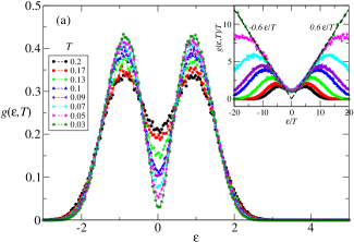
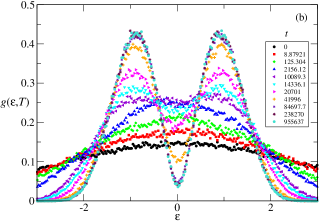
Figure 2: Pseudo-equilibrium (a) and time-dependent (b) single-particle density of states for $L=512$, as function of temperature and time respectively. Data in (b) corresponds to $T=0.04$.

We implemented the above algorithm in CUDA CUD (2013) for the case in which the sites belong to a lattice with toroidal boundary conditions. In this case $\Gamma^{T}_{ij}$ only depends on $r_{ij}$ (thus $\Gamma=N\sum_{i}\Gamma^{T}_{ij}$) hence the “tower” is much smaller than for the model with random sites Tsigankov et al. (2003). At each iteration we need $3M$ random numbers (to choose $i_{k}$, $r_{i_{k}j_{k}}$, and to accept the hops), which requires a random number generator (RNG) able to generate a large number of uncorrelated random sequences in parallel. The code uses functions of our own and the open-source libraries Thrust THR (2013) (for generic parallel transformations) and Philox from Random123 Salmon et al. (2011) (a GPU-suitable RNG). The code also exploits the “embarrassing parallelism” of the local energy update: we distribute the update on $N$ parallel threads, where the $k$-th thread updates the local energy on lattice site $k$.

4 Results for the lattice model in two dimensions

We simulated two-dimensional square lattices with $N=L^{2}$ sites, for $L=64,128,256,512,1024,2048$, setting $\nu=1/2$, $\xi=1$, $W=1$, and $E=T/10$. We use toroidal boundary conditions in both directions, and adopt the minimal image convention for $r_{ij}$ and $\Delta x_{ij}$. We do not allow hops larger than $L/2$ (in our simulations, the typical hopping length is much shorter than $L/2$ anyway). To recover cgs units from the numerical data below, the dimensionless quantities $\{H,T,t,E,P,\sigma\}$ must be multiplied respectively by $\{e^{2}/(\kappa a),e^{2}/(\kappa ak_{B}),\tau_{0},e/(\kappa a^{2}),ea,a^{3-D}\kappa/\tau_{0}\}$, where $e$ is the electron charge and $\kappa$ is the dielectric constant of the lattice.

To validate the code, we start by analyzing the single-particle density of states, defined as the normalized histogram $g(\epsilon,T)=\sum_{k}\delta_{\Delta\epsilon}(\epsilon-\epsilon_{k})$, for a given binning size $\Delta\epsilon$. In Fig.2(a) we show $g(\epsilon,T)$ in the steady state for different temperatures and $L=512$. As shown in the inset, in the Coulomb gap region the data can be rescaled as $g(\epsilon,T)=Tf(\epsilon/T)$, and are well fitted by $g(\epsilon,T)=c|\epsilon|$ for small $|\epsilon|$, with $c=0.62$. The prefactor is consistent with the theoretical estimate Efros (1976) $c=2/\pi$ but is larger than the estimate $c=0.40$ obtained with the parallel tempering MC algorithm goe (2012), which allows many-electron rearrangements and thus can reach lower energies then the single-particle KMC, even if the latter seems to have reached a steady state, as shown in Fig.2(b)).

Next, we analyze the conductivity. The inset of Fig.3(a) shows how, starting from a random configuration, after a transient time the polarization grows linearly in time, and a stationary conductivity can be estimated as $\sigma_{0}=P/(NEt)$ for large $t$. Further relaxation of the conductivity at larger times cannot be discarded, but should be neglibible for time scales a few times larger than the transient time. Our data for $\sigma_{0}(T)$, shown in Fig.3(b), agree with Ref.Tsigankov and Efros (2002) up to a factor two. The data are well fitted by the Efros-Shklovskii law $\sigma_{0}=bT^{-\lambda}\exp[-(T_{0}/T)^{1/2}]$ assuming $\lambda=1$, which gives $T_{0}=6.2,b=2.7$. However, the choice $\lambda=2$ fits equally well the data for $T<0.25$, giving $T_{0}=9.3,b=1.7$.

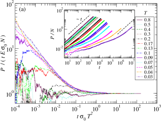
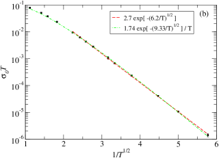
Figure 3: (a) Inset: time evolution of the polarization starting from a random initial configuration at different temperatures for $L=512$. The steady-state conductivity $\sigma_{0}=\lim_{t\to\infty}(dP/dt)/(NE)$ is reached after a transient time $\tau\approx 1/(T^{2}\sigma_{0})$. Main figure: same data rescaled as a function of $t/\tau$. In this figure we use a deterministic time increment $\Delta t=m/\Gamma$. Using a stochastic increment does not produce any appreciable difference. (b) Fit to the Efros-Shklovskii law $\sigma_{0}=bT^{-\lambda}\exp[-(T_{0}/T)^{1/2}]$ for $\lambda=1,2$.

As shown in the main figure, the time evolution of $P(t)$ at different temperatures can be collapsed very well onto a single curve by rescaling the time with a characteristic transient time $\tau\sim(\sigma_{0}T^{2})^{-1}$. This suggests a scaling relation

$$\sigma(t,T)=\sigma_{0}(T)f(t\sigma_{o}(T)T^{2})\,.$$ (4)

We checked that finite-size effects on $P(t)$ are negligible. The proportionality of $\tau$ to $\sigma_{0}^{-1}$ is to be expected Tsigankov et al. (2003); Bergli and Galperin (2012), since the typical hopping time of the current-carrying hops is $\sim\exp[(T_{0}/T)^{1/2}]$. A discussion of the significance of the factor $T^{2}$ (both in $\tau$ and, possibly, in the Efros-Shklovskii law) is outside the scope of this paper, but we note that using the scaling variable $t/(\sigma_{0}T)$ we obtain a much worse data collapse (not shown). It is interesting to compare Eq.(4) with the scaling $\sigma(\omega,T)=\sigma_{0}(T)f(\omega/T\sigma_{0}(T))$ for the low-frequency ac conductivity found in Ref.ber (2014).

5 Code performance

In this section we compare the performance of our parallel GPU code with that of a serial CPU implementation of the mixed algorithm. In both cases, the wall-clock computing time required to execute a hop is the sum of two main contributions: the rejection time, $W_{R}$, spent proposing and rejecting hops until one is accepted, and the update time, $W_{U}$, spent updating the $N$ local energies after a hop is executed. As discussed earlier, aside from hardware-related corrections we expect $W_{R}\propto A^{-1}\log L$ for the CPU code and $W_{R}\propto(AM)^{-1}\log L$ for the GPU code running on $M$ threads, where the acceptance $A$ increases with the temperature and the $\log L$ factor comes from the tower-sampling. $W_{U}$ is independent of the temperature and the configuration, and we expect $W_{U}\propto L^{2}$. In the parallel implementation, nevertheless, this will hold only at large enough $L$ (when the hardware occupancy saturates), while at smaller sizes the scaling will be sublinear in $L^{2}$, and even constant for very small sizes. In the Coulomb glass, most excitations active at low $T$ are dipoles (short electron-hole pairs). In 2D the density of states of dipoles at low energy is constant, which implies $A\propto T$ in the steady state (indeed we find $A\approx 0.03\,T$). Hence, the overall computing time will be dominated by $W_{R}$ for temperatures below a certain threshold that decreases with $L$ as $\log L/L^{2}$, and by $W_{U}$ above the threshold.

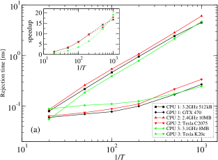
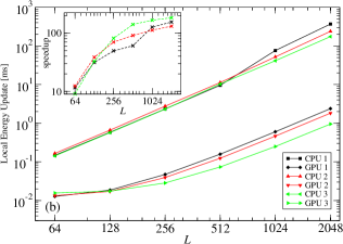
Figure 4: Computing time [ms] per executed hop for the serial and parallel codes in three different CPU+GPU platforms. We benchmark a fair serial single CPU core implementation against our parallel GPU implementation (with the same CPU core as host), both with double precision floating point operations. (a) Temperature dependence of the average rejection time ($W_{R}$) for $L=256$. (b) Size dependence of the average update time ($W_{U}$) of the $N=L^{2}$ local energies. The insets show the speedup of the GPU over the CPU implementation. While the speedup starts to saturate with $L$ in (b), it is still strongly growing with $1/T$ in (a).

To see how well the above estimates hold in practice, in Fig.4(a) we show the temperature dependence of $W_{R}$ for the CPU and GPU codes in the steady state for $L=256$ (the dependence on $L$ is very weak). For the CPU code, we see roughly $W_{R}\propto 1/T$, as expected. For the GPU code we used a number of threads close to the optimal value $M^{*}\approx A^{-1}$. Hence, at moderate temperatures where $M^{*}$ is not too large, $W_{R}\propto(M^{*}A)^{-1}$ is almost independent of $T$, as expected. At very low $T$, $M^{*}$ is large enough to saturate the maximum number of concurrent threads and thus $W_{R}$ increases with $1/T$, although less than linearly since the GPU can still save time by hiding memory latency. Therefore, the relative performance of the GPU vs the CPU codes, shown in the inset, is consistent with the expected linear behavior in $1/T$.

In Fig.4(b) we compare the size dependence of $W_{U}$ for the GPU and CPU implementations. As expected, for the CPU we observe $W_{U}\propto L^{2}$ while for the GPU, using $L^{2}$ threads, $W_{U}$ is almost constant for small $L$ and grows for large $L$. Interestingly, the increase is still sublinear even when $L^{2}$ is several times larger than the number of physical cores, due to the efficient internal thread scheduling. Consequently the speedup, which is already substantial even for relatively small sizes, increases with $L$ and exceeds two orders of magnitude at $L=2048$, without quite saturating yet.

The overall computing time per executed hop of the GPU code is basically the sum of $W_{R}$ and $W_{U}$. For example, for the platform CPU3+GPU3 (see Fig.4 for details) the overall time ranges from 0.1 ms ($L$=64) to 1.04 ms ($L$=2048) at $T=0.05$, representing speedups of 1.7x to 179x respect to the serial code, and 0.27 ms ($L$=64) to 1.23 ms ($L$=2048) at $T=0.001$, representing speedups of 15x to 157x. Nevertheless, note that these speedup factors depend on the particular serial implementation and hardware.

In order to see in what regime of $T$ and $L$ the GPU code may be useful in practice, it is illustrative to estimate the physical time we can simulate in, say, a ten-day run. While this time is independent of $T$ for the CPU code, according to the previous discussion it scales as $1/T$ for the GPU code for low enough $T$. This is confirmed in Fig.1(b), where we also show the transient time $\tau=1/(\sigma_{0}T^{2})$ for the establishment of a steady-state conductivity. Clearly, since $\tau$ grows much faster than the speedup as $T$ decreases, even the GPU code cannot reach the steady state at very low $T$. At the temperatures at which we can reach the steady state, the typical hopping length $r\sim(\xi/4)(T_{0}/T)^{1/2}$ is less than ten lattice spacings. Hence, for the purpose of measuring the conductivity it is preferable to average over many samples at intermediate $L$, rather than a few samples at large $L$. Large samples, for which the GPU code is significantly advantageous, might be useful for studying the large-scale geometry of the conducting paths, for instance.

It is worth noting that the GPU code should be significantly more advantageous in 3D than in 2D, because (i) $N$ increases more rapidly with $L$, and (ii) both $T_{0}$ and the dipole density of states of dipoles are smaller in 3D, so in the VRH regime the acceptance rate is even lower. It is also straightforward to incorporate multiple-electron hops in our GPU code. Since these hops have even lower acceptance rate, we expect the speedup to be substantial.

6 Conclusions

We have presented a novel parallel KMC technique for simulating the Coulomb glass hopping conduction. It allows to simulate larger systems and longer times than its serial counterpart, with speedups over 100x for relatively large system sizes in two dimensions. This might be helpful for studying features involving larger length-scales. In 2D, we find that the short-time relaxation of the conductivity at different temperatures is well described by a single scaling curve. Finally, our current implementation can be easily extended to higher dimensions, multiple occupation, and multi-electron hops. For these extensions we can expect an even larger speedup with respect to the mathematically equivalent serial implementation. The code is available to download, modify and use under GNU GPL 3.0 at cod (2014).

References

- Tsigankov and Efros (2002) D. N. Tsigankov and A. L. Efros, Phys. Rev. Lett. 88, 176602 (2002).
- Tsigankov et al. (2003) D. N. Tsigankov, E. Pazy, B. D. Laikhtman, and A. L. Efros, Phys. Rev. B 68, 184205 (2003).
- CUD (2013) https://developer.nvidia.com/what-cuda (2013).
- Niemi and Wheeler (2011) J. Niemi and M. Wheeler, ArXiv e-prints (2011), 1101.4242.
- Bortz et al. (1975) A. Bortz, M. Kalos, and J. Lebowitz, Journal of Computational Physics 17, 10 – 18 (1975), ISSN 0021-9991.
- Efros (1976) A. L. Efros, Journal of Physics C: Solid State Physics 9, 2021 (1976).
- Krauth (2006) W. Krauth, Statistical Mechanics: Algorithms and Computations, Oxford University Press, Oxford, 2006, pp. 33–34.
- THR (2013) Thrust parallel algorithms library, http://thrust.github.com/ (2013).
- Salmon et al. (2011) J. K. Salmon, M. A. Moraes, R. O. Dror, and D. E. Shaw, “Parallel random numbers: as easy as 1, 2, 3,” in Proceedings of 2011 International Conference for High Performance Computing, Networking, Storage and Analysis, SC ’11, ACM, New York, NY, USA, 2011, pp. 16:1–16:12, ISBN 978-1-4503-0771-0.
- goe (2012) M. Goethe and M. Palassini, unpublished; M. Goethe, Ph.D. thesis, University of Barcelona (2012).
- Bergli and Galperin (2012) J. Bergli and Y. M. Galperin, Phys. Rev. B 85, 214202 (2012).
- ber (2014) J. Bergli and Y. M. Galperin, in these Proceedings (2014).
- cod (2014) https://bitbucket.org/ezeferrero/coulomb_glass (2014).