Interpreting broad emission-line variations I : Factors influencing the emission-line response

Abstract

We investigate the sensitivity of the measured broad emission-line responsivity $d\log f_{\rm line}/d\log f_{\rm cont}$ to continuum variations in the context of straw-man BLR geometries of varying size with fixed BLR boundaries, and for which the intrinsic emission-line responsivity is known a priori. We find for a generic emission-line that the measured responsivity $\eta_{\rm eff}$, delay and maximum of the cross-correlation function are correlated for characteristic continuum variability timescales $T_{\rm char}$ less than the maximum delay for that line $\tau_{\rm max}$(line) for a particular choice of BLR geometry and observer orientation. The above correlations are manifestations of geometric dilution arising from reverberation effects within the spatially extended BLR. When present, geometric dilution reduces the measured responsivity, delay and maximum of the cross-correlation function. Conversely, geometric dilution is minimised if $T_{\rm char}\geq\tau_{\rm max}$(line). We also find that the measured responsivity and delay show a strong dependence on light-curve duration, with shorter campaigns resulting in smaller than expected values, and only a weak dependence on sampling rate (for irregularly sampled data).

The observed strong negative correlation between continuum level and line responsivity found in previous studies cannot be explained by differences in the sampling pattern, light-curve duration or in terms of purely geometrical effects. To explain this and to satisfy the observed positive correlation between continuum luminosity and BLR size in an individual source, the responsivity-weighted radius must increase with increasing continuum luminosity. For a BLR with fixed inner and outer boundaries this requires radial surface emissivity distributions which deviate significantly from a simple power-law, and in such a way that the intrinsic emission-line responsivity increases toward larger BLR radii, in line with photoionisation calculations.

1 Introduction

Determining the geometry and kinematics of the broad emission-line region (hereafter BLR) has been a long sought after goal of Active Galactic Nuclei (AGN) monitoring campaigns. Early campaigns focused on recovery of the 1-d response function $\Psi(\tau)$ for the broad emission-lines, the function which maps the continuum variations onto the line variations as a function of time-delay $\tau$, in an effort at mapping the spatial distribution of the variable line emitting gas. However, it was realised almost from the outset, that the form of the 1-d response functions for diverse BLR geometries are largely degenerate and that $\Psi(\tau)$ is unable to unambiguously pin down the geometry of the BLR gas (Welsh and Horne 1991; Pérez, Robinson and de la Fuente 1992b). Despite this, reverberation mapping has enjoyed enormous success. Even with low quality data, measurement of the delay between the continuum and broad emission-line variations via the cross-correlation function (hereafter CCF), yields with a few assumptions, a measure of the luminosity-weighted size of the line-emitting region. When combined with a measure of the velocity dispersion of the line-emitting gas, and assuming that the BLR gas is virialised, broad line variability data can be used to determine the mass of the central black hole. Indeed RM mass estimates are now available for more than 40 nearby AGN, from which scaling relations have been derived for several UV and optical broad emission-lines allowing access to black hole mass determinations for AGN from single epoch spectra (Kelly and Bechtold 2007; Denney et al. 2009; Shen et al. 2008; Shen and Kelly 2010; Runnoe et al. 2013).

Applying time variability studies to multiple lines in individual sources has proven equally profitable. For the best studied source NGC 5548, reverberation mapping experiments reveal the BLR to be both spatially extended and highly stratified, with a broad range in delays exhibited among lines of differing ionisation stage suggestive of strong gradients in density and/or ionisation (e.g. Netzer and Maoz 1990; Krolik et al. 1991; Clavel et al. 1991; Peterson et al. 1992, 1994, 2002, Korista et al. 1995, and references therein).

The shortest delays ($\sim$ a few days) are measured for the UV high ionisation lines (HILs), (e.g. N v, C iv, He ii). For these lines the recovered 1-d response functions are temporally unresolved (owing to sparse sampling of the UV light-curves), peaking at zero-delay, and declining rapidly on timescales of a few days. This contrasts with the recovered response functions for the LILs. For example, the broad optical recombination lines (H$\alpha$, H$\beta$), have little response at zero delay, instead rising to a peak at $\sim$20 days before declining rapidly toward zero (Horne, Welsh and Peterson 1991; Ferland et al. 1992). While the UV Fe ii emission-lines were found to vary on a similar timescale and with similar amplitude to the Balmer emission-lines (Maoz et al. 1993), for Mg ii and the optical Fe ii lines, the variability amplitude was so small that only a lower limit on the delay was possible (Clavel et al. 1991; Vestergaard and Peterson 2005). Similarly, for C iii], a density sensitive inter-combination line, only a lower limit for the delay is available, suggesting that the characteristic density of the BLR decreases radially outward (Clavel et al. 1991; Krolik et al. 1991).

1.1 The 13 yr ground-based optical monitoring campaign of NGC 5548

Of the $\approx$40 or so nearby AGN with extensive ground-based continuum–emission-line monitoring data, the 13 yr ground-based monitoring campaign on NGC 5548 carried out by the Ohio State University as part of the AGN Watch collaboration remains the de-facto gold standard, both in terms of sampling frequency, campaign duration, and data quality (Peterson et al. 2002 and references therein). While not approaching the signal to noise or sampling frequency available with space-based instruments, the extensive ground-based coverage allows investigation of the emission-line delay and amplitude of response on a season by season basis, and on timescales longer than the BLR dynamical timescale ($\sim$ a few years for NGC 5548), and importantly, their dependence on ionising continuum luminosity.

In Figure 1 we show the galaxy subtracted optical (5100Å) continuum light curve (black points) and the corresponding broad H$\beta$ emission-line light curve (red points) for NGC 5548 after having first corrected for contaminating narrow H$\beta$ emission using the latest values of the (now known to be time-variable on timescales of $<$ 13 years) narrow line contribution to broad H$\beta$ from Peterson et al. (2013). For the purposes of illustration only we have normalised the continuum and emission-line light-curves to their respective mean values. The broad emission-line light-curve clearly follows the continuum light-curve albeit with a small delay (see Peterson et al. 2002, and references therein). In the middle panel we show the galaxy subtracted optical (5100Å) continuum light curve (black points) together with the narrow line subtracted broad H$\beta$ emission-line light-curve, with the latter shifted, on a season by season basis, by the delay (as measured from the centroid of the cross-correlation function, hereafter CCF) between the continuum and broad emission-line light curve, using values taken from Peterson et al. 2002). The continuum and emission-line light curves are well-matched, with the optical continuum light curve displaying larger amplitude variations than the broad emission-line light-curve. In the lower panel of Figure 1 we show the time variable EW of the broad H$\beta$ emission line light-curve. Since the continuum and broad emission-line light-curves are irregularly sampled and the broad emission-line light-curve has been shifted in time, we determine the line EW (the ratio of the line to continuum flux) at the corresponding continuum values by linearly interpolating between nearest neighbour points.

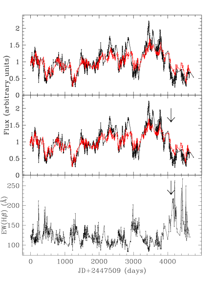
Figure 1: Top panel - the galaxy subtracted optical continuum and narrow line subtracted broad H$\beta$ emission-line light-curve of NGC 5548 as observed during the 13 yr optical monitoring campaign. For clarity both light-curves have first been normalised to their respective mean values (see text for details). Middle panel, as above, but with each season of data corrected for the measured delay between the continuum and emission-line variations. Lower panel - the time-variable EW for broad H$\beta$ as determined from the lag corrected data. The downward arrow indicates the onset of large EW which follows a period of prolonged high continuum and emission-line fluxes (§1.1.)

Figure 1 indicates several key observational features of AGN monitoring campaigns. First, the broad emission-line light-curve correlates well with the optical continuum light curve which not only confirms ionising continuum variations as the key driving mechanism for the broad emission-line variations, but suggests that the continuum variability timescale and BLR size are generally well-matched, and furthermore indicates that the optical continuum may be used as a proxy for the driving UV ionising continuum.

However, when looked at in detail, the broad H$\beta$ emission-line light-curve shows small seasonal shifts (in delay) of varying size relative to the optical continuum light curve, and is somewhat smoother in appearance, displaying smaller amplitude excursions about its mean level. Both of these effects are normally attributed to light-travel time-effects (reverberation) within the spatially extended BLR. Both the continuum–emission-line delay (or lag) and the amplitude of the emission-line variations (the line responsivity, $\eta$) are key components of the broad emission line response function $\Psi(\tau)$, the convolution kernel relating the continuum to broad emission-line variations the recovery of which has been the major goal of AGN monitoring (reverberation mapping, RM) campaigns over the past 25 years.

However, there is a subtlety revealed by the continuum and emission-line light-curves which is often overlooked. When recast in terms of the line EW, it becomes apparent that the line EW for broad H$\beta$ is not constant, but instead varies by a factor of $\approx 2$ over the full 13 yr campaign. Furthermore, the H$\beta$ EW varies inversely with the continuum level, with the largest values occurring during low continuum states and the smallest values occurring during high continuum states. Formally, the measured continuum – broad emission-line fluxes in a given AGN are related by

$$f(H\beta)\propto f_{cont}^{\eta_{\rm eff}}\,,$$ (1)

where $\eta_{\rm eff}$, the power-law index in this relation, measures the effective responsivity of a particular emission-line over the full BLR, modulo a first order correction for the continuum–emission-line delay, which dilutes the signal (geometric dilution) and introduces scatter in the above relation. In terms of the line EW, equation 1 becomes

$$EW(H\beta)=\frac{f(H\beta)}{f_{cont}}\propto f_{cont}^{\eta_{\rm eff}-1}\,.$$ (2)

Since in general we measure a local equivalent width for H$\beta$ using nearby continuum bands (typically 5100Å), this simplified expression ignores the fact that the driving UV continuum may exhibit larger amplitude variations than the optical continuum bands. Values of $\eta_{\rm eff}<1$ may be associated with an intrinsic Baldwin effect (e.g. Kinney et al. 1990; Pogge and Peterson 1992; Gilbert and Peterson 2003; Han et al. 2011) for this line, and the EW(H$\beta$) is indeed found to be inversely correlated with continuum strength, being larger in low continuum states (compare the middle and lower panels of Figure 1), and smaller in high continuum states (Gilbert and Peterson 2003; Goad, Korista and Knigge 2004; Korista and Goad 2004). Since the emission-line EW is a measure of the efficiency with which the BLR gas reprocesses the incident ionising continuum into line emission, this suggests that the continuum re-processing efficiency for H$\beta$ decreases as the ionising continuum strength increases (Korista and Goad 2004). Indeed the measured factor of 2 or more variation in emission-line EW for broad H$\beta$ relative to the optical continuum band in NGC 5548 is in close agreement with the predicted variation in EW(H$\beta$) from photoionisation model calculations (see §3.2 of Korista and Goad 2004). Note that while the continuum re-processing efficiency for a single line may change dramatically with continuum level (for example if $\eta_{\rm eff}<1$, we will observe an intrinsic Baldwin effect), the overall gas re-processing efficiency may remain unchanged if contributions from other lines adjust accordingly (Maoz 1992).

Gilbert and Peterson (2003), and Goad, Korista and Knigge (2004) went on to show that the measured line responsivity $\eta_{\rm eff}$ is not constant, but instead varies with continuum state, being smaller in high continuum states, and larger in low continuum states, a continuum-level dependent emission-line responsivity $\eta_{\rm eff}=\eta_{\rm eff}(L_{\rm cont}(t))$. Since the gas covering fraction is unlikely to correlate strongly with ionising continuum strength, then these observations point towards a physical origin for this effect within the BLR gas. Notice that the largest H$\beta$ EWs in the lower panel of Figure 1 correspond to low continuum states and indicate a higher re-processing efficiency for the line-emitting gas at lower ionising continuum fluxes, as predicted by the photoionisation calculations of Korista and Goad (2004) and equation 2, for $\eta_{\rm eff}<1$.

The large upward and downward excursions in line EW for broad H$\beta$ seen in the lower panel of Figure 1 anti-correlate with continuum level (Goad, Korista and Knigge 2004) and can be explained in terms of (i) a decrease in the continuum re-processing efficiency for H$\beta$ with increased continuum flux as predicted by photoionisation model calculations, a purely local effect (e.g. Korista and Goad 2004, and see §2.1), (ii) the increase in the luminosity-weighted radius with increasing continuum flux which subsequently follows, and which for a given characteristic continuum variability timescale $T_{\rm char}$ results in a larger delay and a lower amplitude emission-line response (here referred to as geometric dilution), and (iii) hysteresis effects arising from the finite light-crossing time of a spatially extended BLR. The larger H$\beta$ EW found for low continuum states, and in particular in those that follow prior high continuum states (for example, as indicated by the arrow in the middle and lower panels of Figure 1) may in part be attributed to hysteresis effects. While an external observer sees the continuum decline with no delay, the line emission arises from gas distributed over a broad range in delay and will be largely dominated by contributions from gas at larger radii responding to the prior (higher) continuum states. Hysteresis in the time-variable line EW may therefore be used as indicator of a spatially extended BLR.

The decline in the continuum re-processing efficiency for a given line with increasing continuum flux, and the resulting increase in the lines’ luminosity-weighted radius with continuum level, are associated with what is commonly referred to as “breathing” (e.g. Goad et al. 1993; Korista and Goad 2004; Cackett and Horne 2006). We explore this effect in a forthcoming paper. Cackett and Horne (2006) provided strong supporting evidence for a breathing BLR in NGC 5548, showing that a time-variable luminosity-dependent response function $\Psi(\tau,L(t))$ provides a better fit to the 13 yr broad H$\beta$ emission-line light curve for this source.

Finally, it is interesting to note that there is an apparent lower limit to the measured time-variable EW for broad H$\beta$ of $\approx$ 80–100 Å (lower panel of Figure 1). Additionally, the time-variable line EW for broad H$\beta$ does not appear invariant to rotation through 180 degreesṪhat is, if we invert the H$\beta$ EW light-curve it does not have the same functional form. This may in part be explained by the general finding that the emission-line responsivity is larger in low continuum states than in high continuum states (e.g. Korista and Goad 2004) and which introduces asymmetry into the line EW variations with continuum level. The apparent bounded behaviour of broad H$\beta$ line EW in high continuum states (and the possibility of a similar bounded behaviour in low continuum states) will be explored further in paper ii.

1.2 The power of photoionisation modelling

Though RM campaigns have been hugely successful, an unambiguous interpretation of the recovered response function remains difficult, because in general, there is no simple one-one relationship between BLR size $R$ and the measured time-delay $\tau$ and because the importance of the local gas physics in determining the amplitude of the emission-line response to continuum variations (the line responsivity) has with a few exceptions been largely overlooked. $\Psi(\tau)$ far from being a simple entity, is determined among other things by the BLR geometry (e.g. sphere, disc, bowl etc), the amplitude and characteristic timescale of the driving continuum light-curve, and by properties of the local gas physics, many of which may themselves vary in a time-dependent manner (for example, as a function of incident continuum flux), all of which are then moderated by our ability to sample the continuum light-curves with sufficient frequency and over long enough duration to mitigate against windowing and sampling effects.

As an exemplar, when taken at face-value the short response timescales found for the HILs in NGC 5548 suggests that these lines either form at small BLR radii, and/or originate close to the line of sight to the observer. However, as their name implies, the HILs require a more intense radiation field for a given gas hydrogen density than the LILs, and therefore the most plausible explanation is that these lines form at small BLR radii, where the radiation field is more intense. Thus an understanding of the photoionisation physics of the gas allows us to distinguish these two scenarios. In a similar fashion, the absence of response in the optical recombination on short timescales, when interpreted geometrically, suggests an absence of gas along the observers line of sight, and by implication a departure from spherical symmetry. However, photoionisation models indicate that the gas emitting the optical hydrogen recombination lines may be optically thick in the line (Ferland et al 1992; O’Brien, Goad and Gondhalekar 1994; Korista and Goad 2004). If so, the absence of response on short timescales, far from indicating an absence of gas, rather suggests that these lines preferentially emerge in the direction of the illuminating source, and therefore the gas remains unseen (for these lines).

The importance of using photoionisation models in the interpretation of broad emission-line variability data is clear (see Goad et al 1993, O’Brien et al 1994,1995; Korista and Goad 2004; Horne, Korista and Goad 2003). In this contribution we use a forward modelling approach to investigate, in a controlled manner, the relative importance of several key factors underpinning the measured emission-line response amplitude (responsivity) and delay (or lag) in response to ionising continuum variations. We begin in §2 by introducing a framework for discussing the emission-line responsivity, distinguishing between the in-situ gas responsivity derived from photoionisation calculations and the effective line responsivity, $\eta_{\rm eff}$, measured by the observers. We then implement an alternative means of measuring $\eta_{\rm eff}$ which doesn’t require a correction for the continuum–emission-line delays (Krolik et al. 1991).

In §3 we introduce a set of controlled reverberation mapping experiments in which we investigate the sensitivity of the measured emission-line response amplitude (the emission-line responsivity $\eta_{\rm eff}$) and emission-line delay $\tau$ to the local gas physics, and BLR geometry (radial extent and geometric configuration), for a range of BLR geometries centred about the BLR size and continuum luminosity normalisation for the well-studied AGN NGC 5548, driven by continuum light-curves with differing characteristic timescales and variability amplitudes, and moderated by the campaign duration and sampling frequency.

In §4 we place our work in context of the observed variability behaviour of the broad H$\beta$ emission-line in NGC 5548 addressing in particular the implications of adopting a spatially and temporally dependent emission-line responsivity (ie. “breathing”) and outline several avenues for further investigation where significant future progress can be made.

2 The emission-line responsivity : definitions

2.1 The in-situ gas responsivity

From a photoionisation modelling perspective we are primarily interested in the in-situ microscopic physics of the line emitting gas and variations in the locally emergent emission-line intensities $F_{\rm line}$, about their equilibrium values resulting from small changes in the incident hydrogen ionising photon flux $\Phi_{\rm H}$, normally referred to as the emission-line responsivity $\eta$. Formally, $\eta$ can be written

$$\eta=\frac{d\log F_{\rm line}}{d\log\Phi_{\rm H}}\,.$$ (3)

and is a measure (locally) of the re-processing efficiency of the line-emitting gas. Assuming that the spectral energy distribution (SED) of the ionising continuum remains constant (to first order), then this may be rewritten as

$$\eta=\frac{d\log EW}{d\log\Phi_{\rm H}}+1\,,$$ (4)

and can be computed directly from photoionisation model grids of line EW as a function of hydrogen gas density $n_{\rm H}$ and hydrogen ionising photon flux $\Phi_{\rm H}$ (e.g. Korista and Goad 2004). This definition of line responsivity $\eta$ is useful because it makes the minimum number of model-dependent assumptions, depending only on the local gas physics (e.g. $\Phi_{\rm H}$, $n_{\rm H}$), and importantly is independent of any assumed geometry, or indeed weighting function describing the run of physical properties with radius. In previous work Korista and Goad (2004) showed that the continuum re-processing efficiencies for the strong optical recombination lines display a general inverse correlation with incident hydrogen ionising photon flux, and consequently their line responsivities tend to increase toward larger BLR radii. Thus for these emission-lines their measured responsivities $\eta_{\rm eff}$ may provide an additional constraint upon the run of gas physical conditions with radius.

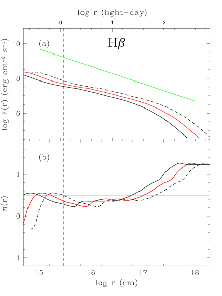
Figure 2: Upper panel - photoionisation model calculations of the radial surface emissivity distribution (solid red line) for broad H$\beta$ for an LOC model and continuum normalisation (see Korista and Goad 2004) appropriate for NGC 5548. Also shown are model low- (solid black line) and high-state (dashed black line) radial surface emissivity distributions for H$\beta$ chosen to represent the peak-to-peak UV continuum variation in this source (factor 8.2 in flux). The green line indicates a radial surface emissivity distribution with power-law index $\gamma=-1$, corresponding to a radial responsivity distribution $\eta(r)=-(\gamma/2)=0.5=constant\;\forall r$ and is used here simply to guide the eye. Lower panel - the equivalent radial responsivity distributions corresponding to changes in their emission-line fluxes about their equilibrium states in response to small continuum variations. The dashed vertical lines indicate the radial extent of our fiducial BLR model.

A radial surface emissivity distribution of an individual emission-line $F_{\rm line}(r)$ (hereafter, $F(r)$) can be determined by summing over a gas density distribution as a function of radial distance $r$ (e.g., see Korista and Goad 2000). From $F(r)$ we can subsequently calculate a radially dependent line responsivity $\eta(r)$ (Goad, O’Brien and Gondhalekar 1993; Korista and Goad 2004). Formally, $\eta(r)$ can be written as

$$\eta(r)=\frac{d\log F(r)}{d\log\Phi_{\rm H}}\,,$$ (5)

and indicates the instantaneous variation in the radial surface emissivity distribution $F(r)$ about its equilibrium value, to small variations in the ionising continuum flux.

Since $\Phi_{\rm H}~{}\propto~{}r^{-2}$, $\eta(r)$ is given by $-0.5d\log F(r)/d\log r$. Example radial responsivity curves $\eta(r)$ for the strong UV and optical broad emission-lines can be found in Goad et al. (1993), and Korista and Goad (2004). For illustration, we show in Figure 2 (upper panel, red line) the radial surface line emissivity for broad H$\beta$ (solid red line) determined for an LOC model of NGC 5548 (Korista and Goad 2004). For broad H$\beta$, $F(r)$ deviates significantly from a single power-law, being better represented by a broken power-law with power-law index $\gamma\approx-0.7$ for radii less than $\approx$25 light-days and steeper than $-2$ for radii greater than $\approx$160 light-days, corresponding to radial responsivities $\eta(r)$, of $\approx 0.35$ and $>1$ respectively (see Figure 2 lower panel, solid red line). For power-law radial surface emissivity distributions $F(r)\propto r^{\gamma}$, $\eta(r)=-(\gamma/2)=constant$ $\forall$ $r$, ie. $\eta(r)$ is a constant both spatially and temporally. However, since in the above example $F(r)$ is not a simple power-law, $\eta(r)$ depends upon the amplitude of the continuum variations, and is therefore luminosity dependent ie. $\eta(r,L_{\rm cont}(t))$.

We can also compute radial surface emissivity distributions $F(r)$ and radial responsivity distributions $\eta(r)$ corresponding to small continuum variations about hypothetical low- (solid black line) and high- (dashed black line) equilibrium continuum states. The radial line responsivity distributions resulting from larger continuum variations, for example when traversing from a low- to high- continuum state, will lie somewhere between the radial responsivity distributions determined for small continuum variations about the low- and high-continuum equilibrium states respectively (see e.g. Korista and Goad (2004) for details).

2.2 Measuring the emission-line responsivity, an observers’ perspective

As mentioned in §1.1 (equation 1), the emission-line responsivity $\eta_{\rm eff}$ is normally calculated from a measurement of the slope in the relation $d\log f_{\rm line}/d\log f_{\rm cont}$, after first applying a gross correction for the average delay $<\tau>$ between the continuum and emission-line variations (e.g. Krolik et al. 1991; Pogge and Peterson 1992; Gilbert and Peterson 2003; Goad, Korista, and Knigge 2004), and having first adequately accounted for contributions from non-varying components, for example, the host galaxy contribution to the continuum light-curve and the contribution of (non-)variable narrow emission-lines to measurements of the broad emission-line flux. Clearly, when determining $\eta_{\rm eff}$, it is important to ensure that the emission-line flux is referenced to the correct (in time) continuum value. Pogge and Peterson (1992) suggested that a global correction for the emission-line delay, $\tau$, is sufficient to enable an accurate recovery of $\eta_{\rm eff}$, demonstrating that data corrected in this fashion shows significantly reduced scatter. However, we note that such a correction introduces its own problems. Krolik et al. (1991) and Pogge and Peterson (1992), when calculating $\eta_{\rm eff}$ for the broad UV emission-lines (as observed with IUE during the 1989 AGN monitoring campaign of the nearby Seyfert 1 galaxy NGC 5548), looked at regularly sampled data, and avoided the need to interpolate their data by shifting their broad emission-line light-curves by lags which were integer multiples of the 4-day sampling rate. By contrast, the unavoidable irregular sampling of the 13 yr ground-based optical light-curves of NGC 5548 required a different approach. Goad, Korista and Knigge (2004) applied the mean delay ($<\tau>$) , as calculated from the centroid of the CCF, for each of the 13 observing seasons of NGC 5548, to the H$\beta$ emission-line light-curve, reconstructing the corresponding optical continuum flux from a weighted average of the continuum points bracketing the observation, using weights and errors derived from the 1st order structure function of the continuum light-curve. They found that for the broad H$\beta$ emission-line, the effective line responsivity $\eta_{\rm eff}$ referenced to the optical continuum, varies between 0.4 – 1.0 over the 13 year optical campaign, with $\eta_{\rm eff}$ inversely correlated with continuum flux, such that the responsivity is generally larger at low continuum flux levels (Goad, Korista and Knigge 2004, their Figure 6). Goad, Korista and Knigge (2004, their Figure 4) suggested that the observed inverse correlation between the broad emission-line responsivity and continuum flux could best be explained in terms of photoionisation models. They predict a larger emission-line responsivity at low incident continuum fluxes, together with a more coherent response of the lines to continuum variations of a given characteristic timescale $T_{\rm char}$ resulting from a smaller responsivity-weighted radius for a BLR of fixed size. A similar inverse correlation between the broad emission-line responsivity and continuum flux has subsequently been found for the broad UV emission-lines in the nearby Seyfert 1 galaxy NGC 4151 (Kong et al. 2006), albeit over a much larger range in continuum flux ($\sim$ factor of 100). This effect which is briefly discussed in §4 will be explored more fully in paper ii.

In previous work, Korista and Goad (2004) investigated how small variations in the ionising continuum about its equilibrium value induces local changes in the emission-line re-processing efficiency leading to a radially dependent emission-line responsivity, $\eta(r)$. Aside from this local effect, there are additional (non-local) effects which act to modify the intrinsic responsivity and give rise to measured values of the responsivity $\eta_{\rm eff}$ which are generally smaller. These non-local effects can be broadly separated into properties of the system which are beyond the control of the observer, and those which relate to how the system is measured and over which the observer has some influence. The former includes for example, the characteristic timescale $T_{\rm char}$ and amplitude $\sigma$ of the variable driving continuum light-curve, that together with a given BLR geometry, size, and observer orientation conspire to dilute the measured responsivity (geometric dilution). The latter includes the duration $T_{\rm dur}$ and sampling rate $\Delta t$ of a particular observing campaign. We show here that $T_{\rm dur}$ should be carefully chosen in order to minimise the effect of windowing on the measured emission-line responsivity. We explore all of these effects for several of the more familiar BLR geometries (e.g. spherical, disc and bowl-shaped BLR geometries).

2.2.1 $F_{\rm var}$, an alternative estimate of $\eta_{\rm eff}$.

Krolik et al. (1991) suggested an alternative and far simpler means of estimating the effective line responsivity, using the ratio of the fractional variability in the line and continuum $F_{\rm var}$(line)$/F_{\rm var}$(cont). For well-sampled long duration light curves (so that all frequencies are suitably covered) $F_{\rm var}$(line)$/F_{\rm var}$(cont) is an unbiased estimator of the slope of the response $\eta_{\rm eff}$ (their §5.2), provided that non-varying components have been adequately accounted for (e.g. the host galaxy contribution to the continuum light-curve and the narrow emission-line contribution to the broad emission-line light curve).

Formally, the fractional variability of a time-series, $F_{\rm var}$ is given as

$$F_{\rm var}=\frac{(\sigma^{2}-\Delta^{2})^{1/2}}{<f>}\,,$$ (6)

where the variance, $\sigma^{2}$, is given by

$$\sigma^{2}=\frac{1}{N-1}\sum_{i=1}^{N}(f_{i}-<f>)^{2}\,,$$ (7)

and $\Delta^{2}$, the mean squared error, is

$$\Delta^{2}=\frac{1}{N}\sum_{i=1}^{N}\Delta_{i}^{2}\,$$ (8)

where $\Delta_{i}$ is the uncertainty on the individual measurements, and the mean, $<f>$, is written as

$$<f>=\frac{1}{N}\sum_{i=1}^{N}f_{i}\,.$$ (9)

One advantage of using $F_{\rm var}$ is that it is relatively straightforward to measure. However its robustness as an unbiased estimator of $\eta_{\rm eff}$ is unsubstantiated, and in particular its sensitivity to geometric dilution and windowing effects remain untested. We discuss this further in §3. In Figure 3 we show a comparison between $\eta_{\rm eff}$ derived from the ratio $F_{\rm var}(\rm line)/F_{\rm var}(\rm cont)$ and that found using the traditional method, $d\log f_{\rm line}/d\log f_{\rm cont}$, both referenced to the optical continuum for each season of the 13 yr NGC 5548 optical monitoring campaign. In each case, the host galaxy contribution to the continuum light-curve and the narrow emission-line contribution to the broad emission-line light curve have been removed, while for the latter, we have also subtracted from each season the mean delay, $<\tau>$, between the continuum and emission-line variations (see Goad, Korista and Knigge 2004 for details). While the two estimates of $\eta_{\rm eff}$ are not identical, they do show a strong correlation, with estimates of $\eta_{\rm eff}$ from the ratio of the fractional variation in the line to the fractional variation in the continuum showing a larger spread.

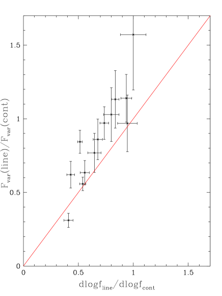
Figure 3: A comparison of the measured broad H$\beta$ emission-line response, for each of the 13 seasons of optical data for NGC 5548. $d\log f_{\rm line}/d\log f_{\rm cont}$ values are taken from Goad, Korista and Knigge (2004) with errors in the slope determined using the bootstrap technique, utilising 10000 simulations, with full replacement.

One obvious drawback to using $F_{\rm var}$ in the determination of $\eta_{\rm eff}$ is that any information about the continuum luminosity is subsequently lost. However, this information may be recovered simply by measuring $F_{\rm var}$ values over light-curve segments corresponding to similar continuum states.

3 Simulations

When considering the measurement of parameters related to BLR variability we must first separate out those effects which are related to the properties of the driving continuum, e.g. amplitude and characteristic variability timescale, from those governed by the local gas physics, the BLR geometry and observer orientation, and the observing window (e.g duration and sampling rate of the continuum and emission-line light curves). The dependence of the continuum–emission-line delay (or lag) on light-curve duration and sampling window for BLRs of varying sizes has been studied elsewhere (e.g. Pérez, Robinson and de la Fuente 1992a; Welsh 1999). To summarise, these studies suggest that the continuum–emission-line delay (or lag) is biased toward small BLR radii, a consequence of finite duration of the observing campaigns and the presence of low frequency power in the light-curves. This effect is more pronounced for the peak of the CCF (the lag) than it is for the CCF centroid. The cross-correlation function is simply the convolution of the continuum autocorrelation function (a symmetric function) with the response function. Thus for light-curves of sufficient duration, the centroid of the CCF (or luminosity-weighted radius) and the centroid of the response function (the responsivity-weighted radius) are equivalent (Penston 1991; Koratkar and Gaskell 1991; Goad, O’Brien and Gondhalekar 1993). Here we study the relationship between the measurement of the emission-line responsivity $\eta_{\rm eff}$ and lag for 3 of the more popular BLR geometries e.g. a sphere, a disc and what we here refer to as our fiducial BLR geometry, a bowl-shaped geometry (see §3.1), within the context of prescribed differences in the characteristic behaviour of the driving continuum light-curve.

3.1 A fiducial BLR model

In previous work, Goad, Korista and Ruff (2012), introduced a new model for the BLR, one in which the BLR gas occupies a region bridging the outer accretion disc with the inner edge of the dusty torus, the surface of which approximates the shape of a bowl. This geometry was motivated by the need to accommodate the deficit of line response exhibited by the recovered 1-d response functions $\Psi(\tau)$ for the optical recombination lines on short timescales, by moving gas away from the observers’ line of sight, while at the same time reconciling the measured delays to the hot dust ($\approx 50$ days) with photoionisation model predictions of the radius at which the dust can form ($\approx 100$ light-days for NGC 5548). Thus, as was first suggested by Netzer and Laor (1993), the outer edge of the BLR is likely largely determined by the distance at which grains can survive. The radially dependent scale-height is maintained by invoking a macro-turbulent velocity field. Such a model is appealing not least because AGN unification schemes which rely on orientation dependent obscuration to distinguish between type i and type ii objects, require viewing angles which peer over the edge of the obscuring torus (ie. down into the bowl) for type i objects.

In brief, the shape of the bowl is characterised in terms of its scale height $H$,

$$H=\beta(r_{x})^{\alpha}\;,$$ (10)

where $r_{x}$ is the projected radial distance along the plane of the accretion disc (ie. $r_{x}=r\sin\phi$, $r$ is the cloud source distance, $\phi$ is the angle between the polar axis and the surface of the bowl), and $\alpha$, $\beta$ are parameters which control the rate at which $H$ increases with $r,\phi$. We adopt a circularised velocity field of the form

$$v_{\rm kep}^{2}=K\frac{r_{x}^{2}}{(r_{x}^{2}+\beta^{2}r_{x}^{2\alpha})^{3/2}}$$ (11)

where $v_{\rm kep}$ is the local Keplerian velocity and $K=GM_{\rm BH}$, where $M_{\rm BH}$ is the mass of the black hole. Using this formulism, when $\alpha=\beta=0$, the geometry resembles a flattened disc with a standard Keplerian velocity field $v_{kep}^{2}=GM_{\rm BH}/r_{x}$. Here we adopt $\alpha=2$ and a time-delay at the outer radius $\tau(r=R_{\rm out})=(r-H)/c=50$ days when viewed face-on, similar to the dust-delay reported for the Seyfert 1 galaxy NGC 5548, yielding $\beta=1/150$. For the chosen black hole mass ($10^{8}$M$\odot$) and continuum luminosity (representative of the mean ionising continuum luminosity for the 13 yr monitoring campaign of NGC 5548), this model BLR spans radial distances of 1.14–100 light-days. We choose a line-of-sight inclination $i=30$ degrees appropriate for the expected inclination of type i objects, which results in a maximum delay at the outer radius of 100 days for this geometry. This we hereafter refer to as the fiducial BLR geometry.

In the following simulations (§3.2–§3.4) we choose for simplicity a radial surface emissivity distribution $F(r)$ for a generic emission–line which is a power-law in radius, $F(r)\propto r^{\gamma}$, with $\gamma$ values of $-1$, and $-2$, roughly spanning the predicted range in power-law index for the radial surface emissivity distribution of broad H$\beta$ over a range of BLR radii (see e.g. Figure 2; Korista and Goad 2004; Goad, Korista and Ruff 2012). For a power-law radial surface emissivity distribution, the radial responsivity distribution $\eta(r)=constant\;\forall r$ (thus $\gamma$ values of $-1$, and $-2$ correspond to $\eta(r)=-(\gamma/2)=0.5$ and $\eta(r)=-(\gamma/2)=1.0$ respectively). In all cases we assume that the BLR boundaries remain fixed at their starting values.

3.2 The driving continuum light-curve

We model the variable ionising UV continuum light-curve as a damped random walk (DRW) in the logarithm of the flux, which has been shown to be a good match to the observed continuum variability of quasars (Uttley et al 2005; Kelly et al. 2009; Kozlowski et al. 2010; MacLeod et al. 2010; Czerny et al. 2003; Zu et al. 2011). For a damped random walk in the logarithm of the flux, the flux distribution function is log-normal by construction.

To simulate the light-curve we first select a random variable with mean $\mu$ and variance $\sigma^{2}T_{\rm char}/2$, where $T_{\rm char}$ is the characteristic timescale (often referred to as the relaxation time or mean reversion timescale) of the DRW, and $\sigma$ represents the variability on timescales much shorter than $T_{\rm char}$. For a given flux $X(s)$, the flux at a later time $t$, $X(t)$ is then constructed piecewise, by selecting in turn a randomly distributed variable with expectation

$$E<X(t)|X(s)>=e^{-\Delta t/T_{\rm char}}(X(s)-\mu)+\mu\,,$$ (12)

and variance

$$Var<X(t)|X(s)>=\frac{\sigma^{2}T_{\rm char}}{2}[1-e^{-2\Delta t/T_{\rm char}}]\,.$$ (13)

By setting $\Delta t=1$ day, the DRW becomes equivalent to an AR(1) process (Kelly et al. 2009). The DRW is controlled by just 3 parameters, $\mu$, $\sigma$, and $T_{\rm char}$. Since in our implementation $X(t),X(s)$ are logarithmic fluxes, $\sigma$ can be written as $\sigma(\log X)$.

Figure 4 panel (i) illustrates 3 DRWs with 1-day sampling and characteristic timescales $T_{\rm char}$ of 10, 40 and 200 days. In each case $\sigma$ has been chosen to produce the same long-term variance in each light-curve ($\sigma^{2}T_{\rm char}/2=0.032$). The transformed light-curves are shown in panel (ii). In panels (iii) and (iv) we illustrate their respective structure functions. In all cases, the structure functions asymptote to twice the variance ($2\sigma^{2}$) on timescales of order the characteristic timescale, $T_{\rm char}$, and to twice the variance of the noise ($2\sigma_{n}^{2}$) on the shortest timescales (not shown).

Equipped with a method for constructing driving continuum light-curves we are now in a position to drive our fiducial BLR geometry to generate model emission-line light-curves and time-variable line profiles from which we can measure the emission-line lag, emission-line responsivity and the fwhm and dispersion of the emission-line profile.

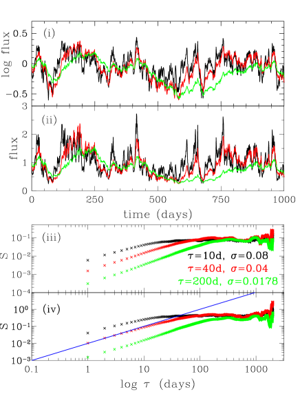
Figure 4: Example continuum light-curves. The light-curves are modelled as DRW in the logarithm of the flux (panel (i)) with constant long-term variance. Colours indicate characteristic timescales of $T_{\rm char}$ of 10 days (red), 40 days (red) and 200 days (green) respectively. Panel (ii) illustrates the transformed light-curves. Panel (iii) shows the structure function for the light-curves shown in panel (i). Panel (iv) indicates the structure function for the transformed light-curves. The solid blue line indicates the expected power-law index for the structure function ($b=1$) appropriate for a Power Density Spectrum (PDS) $P(f)\propto f^{-\alpha}$, with $\alpha=2$, and here $f$ is the frequency.

3.2.1 The effect of light-curve duration and sampling frequency on the measured line response

As far as we are aware there are no extant studies into the effect of light-curve duration and sampling frequency on measurement of the effective emission-line responsivity, $\eta_{\rm eff}$. To remedy this situation, we have performed detailed monte-carlo simulations to probe the effect of campaign length and sampling frequency on the determination of $\eta_{\rm eff}$. We employ two different techniques for measurement of $\eta_{\rm eff}$, thereby allowing us to compare their relative robustness to light-curve duration and sampling patterns.

We determine the emission-line light curve by driving our fiducial BLR model as described in section §3.1 with a simulated DRW (§3.2) in the logarithm of the flux assuming a locally linear response approximation. Thus for these simulations measured differences in the emission-line response (e.g. mean delay, and line responsivity $\eta_{\rm eff}$ are governed only by differences in the characteristics of the driving continuum light-curve ($\sigma$, $T_{\rm char}$).

Unless otherwise specified we adopt a characteristic continuum variability timescale $T_{\rm char}=40$ days, similar to that measured for the UV continuum in the well-studied Seyfert 1 galaxy NGC 5548 (Collier et al. 2001) and $\sigma=0.04$, giving a long-term variance $\sigma^{2}T_{\rm char}/2$ = 0.032.

3.2.2 Duration

First we examine the effect of performing different duration observing campaigns on the measured emission-line responsivity, assuming uniform 1-day sampling for input continuum light-curves spanning durations of $T_{\rm dur}=100$, 200, 500, 1000 and 1500 days. For each input continuum and resultant emission-line light-curve combination, we add a random noise component drawn from a random Gaussian deviate with $\sigma=0.01*f$, where $f$ is the flux. Each point is then assigned an error bar in a similar fashion.

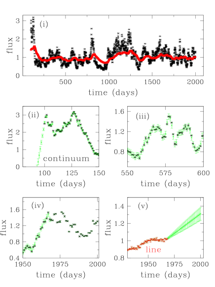
Figure 5: Panel (i) – model continuum (black) and emission-line (red) light-curves. Panels (ii)–(iv) - original continuum data points (black) and estimated continuum values (green points) corresponding to the lag-corrected emission-line epochs with values determined by interpolating between the bracketing continuum points and errors estimated from the structure function of the continuum light-curve. Panel (ii) indicates the extrapolation of the continuum at shifted line epochs prior to the start of the campaign. Panels (iii) and (iv) indicate interpolated continuum points (green). Panel (v) shows the extrapolated line light-curve (green points) for those continuum epochs at the end of the campaign (panel (iv)) for which there are no corresponding line data. Here we have assumed a power-law radial emissivity law $F(r)\propto r^{\gamma}$, with $\gamma=-1$, and $\eta_{\rm eff}=-(\gamma/2)=0.5$

We calculate the effective emission-line responsivity $\eta_{\rm eff}$ using the two methods described in §2, thereby allowing us to compare their relative merits. The simplest method for calculating $\eta_{\rm eff}$ utilises the ratio of the fractional variance in the emission-line relative to the fractional variance in the continuum (see §2.2.1). For each continuum–emission-line light-curve combination we determine $\eta_{\rm eff}=F_{\rm var}(\rm line)/F_{\rm var}(\rm cont)$, and its dispersion $\sigma$, from the centroid and dispersion of the distribution function of $\eta_{\rm eff}$ computed from bootstrap resampling of the input continuum and emission-line light-curves (using 10,000 trials with full replacement). Note that for real data, each light-curve should first be corrected for contaminating non-varying components, for example the host galaxy contribution to the continuum light-curve, and the narrow emission-line contribution to the broad emission-line fluxes. While the narrow-line contribution to the broad emission-line flux is relatively straightforward to measure, particularly if low-state spectra exist, contributions from stellar light in the host-galaxy to the measured continuum flux are generally more problematic (Bentz et al. 2006). However, host galaxy contamination of the continuum light-curve can be mitigated if UV continuum measurements are available, since the contribution of stellar light to the UV continuum is modest at best.

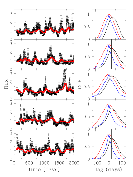
Figure 6: Left-hand panels - Example continuum (black points) and model emission-line light-curves (red points), see text for details. Right-hand panels - the corresponding cross-correlation function (black line), continuum auto-correlation function (blue line) and line auto-correlation function (red line). The vertical solid line indicates the CCF peak (or lag), the vertical dashed line the CCF centroid. Note that the measured lag (CCF peak of centroid) is sensitive to the form of the driving continuum light-curve, as denoted by the continuum ACF. Here we have assumed a power-law radial emissivity law $F(r)\propto r^{\gamma}$, with $\gamma=-1$, and $\eta_{\rm eff}=-(\gamma/2)=0.5$.

For the second method, we adopt the approach used in Goad, Korista and Knigge (2004), using $d\log f_{\rm line}/d\log f_{\rm cont}$ to determine $\eta_{\rm eff}$, having first corrected for contaminating narrow-line contributions to the broad emission-line flux and the host galaxy contribution to the continuum flux, and the “average delay” between the continuum and emission-line light-curves, using their respective structure functions to estimate the uncertainties on interpolated and extrapolated points (see Figure 5). Thus for each continuum–emission-line light-curve combination we first compute the centroid of the cross-correlation function (hereafter, CCF) between the continuum and emission-line light-curve, measured above a CCF threshold of 0.6 of the peak correlation. Example model continuum and emission-line light-curves and their corresponding CCFs are shown in Figure 6 for an assumed power-law radial surface emissivity distribution $F(r)\propto r^{\gamma}$, with $\gamma=-1$, corresponding to $\eta_{\rm eff}=-(\gamma/2)=0.5$ (e.g. as indicated by the green lines in Figure 2). Note that even for a characteristic damping timescale of 40 days for the driving UV continuum, the form of the continuum ACF varies considerably, depending on the nature of the continuum variability over the campaign duration.

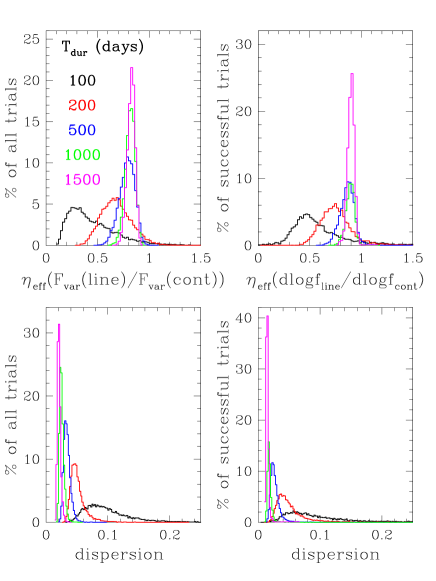
Figure 7: Upper panels - the distribution function for $\eta_{\rm eff}$ as measured using the ratio of the variance in the line relative to the variance in the continuum (upper left), and from the ratio $d\log f_{\rm line}/d\log f_{\rm cont}$ after first correcting for the delay between the continuum and emission-line variations (see text for details). Colours represent results from simulated light-curves with durations of 100 (black), 200 (red), 500 (blue), 1000 (green), and 1500 (magenta) days, each sampled at 1-day intervals. Lower panels – the corresponding distribution function for the dispersion on $\eta_{\rm eff}$ from each of the simulated light-curves measured using bootstrap resampling of the light-curves with full replacement. Here we have assumed a power-law radial surface emissivity distribution $F(r)\propto r^{\gamma}$, with $\gamma=-2$, and $\eta_{\rm eff}=-(\gamma/2)=1$.

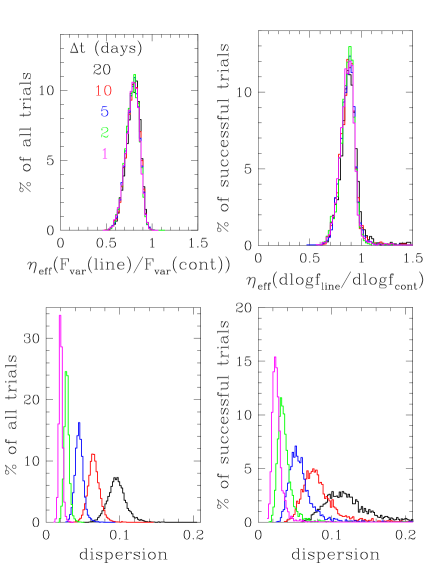
Figure 8: Effect of the sampling pattern on the measured response $\eta_{\rm eff}$. For a fixed light-curve durations of 500 days, we resample the continuum and emission-line light-curves a fixed number of times. The distribution in $\eta_{\rm eff}$ as determined from measurements of the ratio of the fractional variation in the line relative to the fraction variation in the continuum for 10,000 simulated light–curves, is unaffected by changes in the sampling rate, for fixed duration light-curve (upper left-panel). However, the dispersion in the measured slope determined from bootstrap resampling, increases significantly at lower sampling rates. Here we have assumed a power-law radial surface emissivity distribution $F(r)\propto r^{\gamma}$, with $\gamma=-2$, and $\eta_{\rm eff}=-(\gamma/2)=1$.

We then shift the emission-line light-curve by the measured delay (the CCF centroid), and reconstruct the continuum light-curve at the corresponding times by interpolation, with flux uncertainties determined directly from the structure function. After applying the shift to the emission-line light curve, there will be no continuum points corresponding to the first few line points and conversely no emission-line measurements corresponding to the last few continuum points. These are determined by extrapolation with uncertainties determined from their respective structure functions. In our implementation, we construct structure functions for both line and continuum light-curves, which are then smoothed using a Savitzky-Golay filter (Press et al. 1992), this effectively smooths the data without any loss of information.

The effective line responsivity, $\eta_{\rm eff}$, the power-law index relating the continuum and emission-line luminosities (equation 1), the quantity of most interest to observers, is determined from least-squares fitting with errors in both $x$ and $y$, with an error estimate (1$\sigma$ uncertainty) in individual slope determinations determined from bootstrap resampling of the original data with full replacement (10,000 trials). Thus for each continuum–emission-line light curve combination we have a single estimate of $\eta_{\rm eff}$ and its associated uncertainty $\sigma$. The whole procedure is then repeated for 10,000 realisations of the driving continuum light-curve. From these we can compute the distribution functions for $\eta_{\rm eff}$ and $\sigma$. The results of our simulations are shown in Figure 7, for (i) $\eta_{\rm eff}$ as determined from the ratio of the fractional variance in the line relative to the fractional variance in the continuum (upper left panel), and (ii) $\eta_{\rm eff}$ as determined from $d\log f_{\rm line}/d\log f_{\rm cont}$ (upper right panel). The lower panels indicate the corresponding distribution functions for the dispersion on the individual measurements, determined from the bootstrap method. The distribution functions only indicate successful trials, which for the second method depends on whether or not measurement of the CCF centroid meets the required threshold of 0.6 between the pre-specified minimum and maximum delays.

Our simulations indicate that both methods used in the determination of $\eta_{\rm eff}$ yield similar results, suggesting that either method may be employed to estimate $\eta_{\rm eff}$ from observational data (Figure 7, upper panels). However, Figure 7 also indicates that even with a 1500 day light-curve with daily sampling, the measured responsivity $\eta_{\rm eff}$, with a range of $0.7<\eta_{\rm eff}<1$ is already less than the input value. This we attribute to geometric dilution of the continuum variations by the spatially extended BLR. We explore this further in §3.3. Moreover, for our chosen BLR model and driving continuum light-curve large variations in $\eta_{\rm eff}$ can be found for light-curve durations shorter than 500 days. In particular, for the light-curve durations of $\sim$100 days, the distribution in $\eta_{\rm eff}$ is both significantly displaced (factor of 2 or more) from the expected value (in the absence of geometric dilution $\eta_{\rm eff}=1.0$ for power-law radial surface emissivity distribution of slope $\gamma=-2$), and becomes highly skewed, with an extended tail toward large $\eta_{\rm eff}$ values. In addition the typical uncertainty on any single measurement also increases as the campaign duration decreases (lower panels). This suggests that campaign durations of a factor of a few longer than the width of the continuum auto-correlation function (ACF) are required in order to remove the influence of windowing effects on the measured value of $\eta_{\rm eff}$ and reduce its uncertainty. Collier et al. (2001) and Horne et al. (2002) showed that accurate recovery of the emission-line response function also requires high cadence long duration monitoring campaigns. We note that if instead we had used a substantially smaller (more compact) BLR, then the impact of campaign duration on the measured responsivity $\eta_{\rm eff}$ and delay $\tau$ would be significantly reduced, particularly for short campaign durations.

We note that for the models described here $\eta_{\rm eff}$ will not in general correlate with continuum level. This arises because for simple power-law radial surface emissivity distributions $F(r)\propto r^{\gamma}$, and therefore $\eta(r)=-(\gamma/2)=constant\;\forall r$, while the boundaries of our model BLR are fixed both spatially and temporally. For our chosen driving continuum, the mean ratio between the maximum and minimum flux is $10\pm 3$ (based on 10,000 simulated light-curves), similar to the range measured for the optical continuum light-curve of NGC 5548 during the 13 yr ground-based monitoring campaign of this source.

3.2.3 Effect of sampling window

Observations from the ground rarely (if ever) approach regular sampling. To illustrate the effect of the sampling pattern on the measured responsivity, we adopt a 500 day light-curve as a baseline. For each 500 day continuum and emission-line light-curve we randomly select an integer number of points with replacement, the rest are then discarded. We then follow the procedure above to determine $\eta_{\rm eff}$. We aim for mean sampling rates of 1,2, 5, 10 and 20 days (equivalent to 500, 250, 100, 50, and 25 points respectively). Figure 8 shows the results of these simulations. Reducing the sampling rate does not significantly alter the distribution function for $\eta_{\rm eff}$. However, the mean dispersion on an individual measurement, increases significantly as the number of sampling points is reduced (Figure 8 lower panel). Note that the dispersion on a single measurement (from bootstrap resampling) is smaller than the dispersion on $\eta_{\rm eff}$ from different realisations of the same process. Thus our simulations demonstrate that both methods of measuring $\eta_{\rm eff}$ are robust to low sampling rates, though the error in an individual measurement will increase as the sampling rate decreases.

Figure 9: Panels (i)–(iii) – the variation in CCF lag, CCF centroid and emission-line responsivity $\eta_{\rm eff}$ as a function of characteristic timescale $T_{\rm char}$ for driving continuum light-curves with a fixed short-timescale variability amplitude $\sigma=0.04$. Panels (iv)–(vi) – the variation in CCF lag, CCF centroid and emission-line responsivity $\eta_{\rm eff}$ as a function of $T_{\rm char}$ for fixed long-term variance $\sigma^{2}T_{\rm char}/2$. Panels (vii)–(ix) – the variation in CCF lag, CCF centroid and emission-line responsivity $\eta_{\rm eff}$ for fixed $T_{\rm char}$ and varying $\sigma$. The dashed horizontal lines in panels (ii), (v) and (viii) represent the centroid of the 1-d response function. The dashed horizontal lines in panels (iii),(vi) and (ix) indicate the expected responsivity in the absence of geometric dilution. The dashed vertical line in panels (vii), (viii) and (ix) represents a plausible upper limit to the short-timescale variability amplitude. In all cases we assume $F(r)\propto r^{\gamma}$, with $\gamma=-2$, and $\eta_{\rm eff}=-(\gamma/2)=1$.

In summary, provided that the sampling rate is irregular, so that both low and high frequency variations are adequately sampled, the measured line responsivity $\eta_{\rm eff}$‘ is most sensitive to the duration of the observing campaign. In particular, for campaigns which are shorter than a few times the light crossing time of the outer boundary of our fiducial BLR ($\sim$100 days), $\eta_{\rm eff}$ can deviate significantly from its expected value of 1.0, being generally biased toward smaller values. This result can be used to inform the design of future reverberation mapping experiments of individual sources.

3.2.4 The dependence of emission-line lag and emission-line responsivity on $T_{\rm char}$, $\sigma$

To test the sensitivity of our measurements of the CCF peak, CCF centroid and line responsivity $\eta_{\rm eff}$ to those parameters which control the short- and long-term variability of the driving continuum light-curve (namely $\sigma$, $T_{\rm char}$) we have simulated sets of fake continuum light-curves, with (i) constant $\sigma$, (ii) constant $T_{\rm char}$, and (iii) constant long-term variance ($\sigma^{2}T_{\rm char}/2$), and assuming fixed BLR boundaries. Our choice of power-law radial surface emissivities and fixed BLR boundaries allows us to cleanly isolate the effect of these parameters on the measured lag and responsivity, from those effects associated with “breathing”, since under these conditions no breathing can occur.

For models (i) and (iii) we vary $T_{\rm char}$ from 10–400 days, encompassing the range in characteristic timescales for the continuum variability of a typical Seyfert 1 galaxy. At each value we generate 100 simulated light-curves sampled at 1 day intervals and with a duration of $T_{\rm dur}=2000$ days, more than long enough to avoid sampling and windowing effects (§3.2.2–§3.2.3). We then drive our fiducial BLR model, and generate a corresponding emission-line light-curve. We add a random Gaussian deviate to simulate noise and assign a random error again drawn from Gaussian distribution with dispersion $\sigma$ equivalent to 1% of the flux at that epoch. For each continuum–emission-line light curve pair we then estimate the CCF peak and CCF centroid (for the latter using a threshold of 60% of the CCF peak), using the implementation of Gaskell and Peterson (1987), interpolating in both light-curves. The emission-line responsivity $\eta_{\rm eff}$ we estimate from the ratio of the fractional variation in the line to the fractional variation in the continuum (§2), with an error estimate determined from bootstrap resampling. The results of this analysis are shown in Figure 9. Here, the points and their error bars represent the centroid and 1$\sigma$ dispersion of the distribution in values determined from 100 simulated light-curves.

For constant $\sigma$ and $T_{\rm char}\geq 100$ days (the maximum delay at the outer radius for our fiducial BLR geometry when viewed at an inclination of 30 degrees), both the CCF peak, CCF centroid and the maximum of the continuum–emission line cross-correlation coefficient are constant (Figure 9 panels (i)–(ii)) and decline sharply for smaller $T_{\rm char}$. Similarly, the effective line responsivity $\eta_{\rm eff}$, is also constant for large $T_{\rm char}$, though slightly smaller than the expected value of 1.0 in the absence of geometric dilution for our chosen emissivity law, and again declines sharply as $T_{\rm char}$ is reduced (see e.g. panel (iii)). Panels (iv)–(vi) of Figure 9 show the variation in each of the measured parameters for fixed long-term variance. As with panels (i)–(iii), each of the parameters is constant for characteristic timescales longer than 100 days and declines rapidly for timescales that are shorter than this. Panels (vii)–(ix) of Figure 9 suggest that the variation in the CCF peak , CCF centroid and line responsivity $\eta_{\rm eff}$ are independent of $\sigma$ for small $\sigma$ ($\sigma$ values larger than $\sigma\sim 0.06$ produce driving continuum light-curves which undergo large amplitude short-timescale variations which are likely unphysical).

Thus in the absence of windowing effects (ie. for light-curves of significantly long duration), and for a simple power-law radial surface emissivity distribution, the measured line responsivity $\eta_{\rm eff}$ and delay are determined by the characteristic timescale of the driving continuum light-curve $T_{\rm char}$ in relation to the the maximum delay at the outer radius for a particular line, $\tau_{\rm max}$(line), given the geometry and observer line of sight inclination. If $T_{\rm char}$ is small compared to $\tau_{\rm max}$(line), then the continuum signal is significantly diluted (geometric dilution), resulting in small $\eta_{\rm eff}$ and smaller delays (e.g. Figure 9, panels (i)–(vi)). Conversely, geometric dilution is minimised if $T_{\rm char}\geq\tau_{\rm max}$(line).

Note that if we had instead chosen a flatter emissivity distribution (e.g. $\gamma=-1$), the measured responsivity would also be reduced because (i) locally the responsivity is smaller ($\eta(r)=-(\gamma/2)=0.5$), and (ii) the larger responsivity-weighted radius resulting from the flatter emissivity distribution would reduce the coherence of the continuum–emission-line variations resulting in larger CCF centroids and lags. Thus for a flatter radial surface emissivity distribution, the knee in the relation shown in panels (iii) and (vi) of Figure 9, would move down and towards the right. Again, for $T_{\rm char}\geq\tau_{\rm max}$(line) geometric dilution is minimised.

Figure 9 indicates that the dependence of the CCF centroid, CCF lag and $\eta_{\rm eff}$ on $T_{\rm char}$ for $T_{\rm char}\leq\tau_{\rm max}$(line) are broadly similar (cf. panels (i)–(iii)). If we take the measured CCF centroid and CCF lag and plot them against $\eta_{\rm eff}$ (for a fixed $T_{\rm char}$), we find that they follow a simple linear relation of the form $\eta_{\rm eff}=m\tau+k$, with coefficients $m=0.038$, $k=0.343$ and $m=0.0948$, $k=0.280$ for the CCF centroid and lag respectively. This suggests that $T_{\rm char}$ determines the extent to which a BLR of fixed radial extent is probed by the continuum variations, and that this in turn sets the value of $\eta_{\rm eff}$. We expand upon the impact of a particular choice of BLR geometry and BLR size in determining the measured responsivity and delay for fixed $T_{\rm char}$ in the following section.

As a general point of interest, we note that if among the general AGN population there exists, for a fixed continuum luminosity, a range in BLR sizes and characteristic continuum variability timescales $T_{\rm char}$ then the varying degrees of geometric dilution exhibited by the AGN population will introduce significant scatter into the BLR size–luminosity relation.

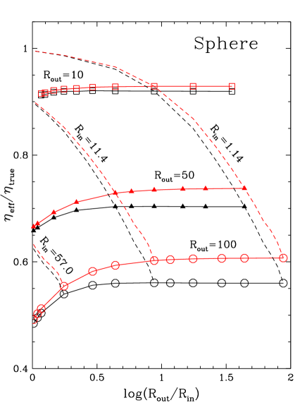
Figure 10: $\eta_{\rm eff}/\eta_{\rm true}$ as a function of $R_{\rm out}/R_{\rm in}$ for a spherical geometry and fixed $R_{\rm out}$ of 100 (open circles), 50 (filled triangles) and 10 (open squares) light-days. Also shown (dashed lines), are $\eta_{\rm eff}/\eta_{\rm true}$ as a function of $R_{\rm out}/R_{\rm in}$ for fixed $R_{\rm in}$ of 1.14, 11.4 and 57.0 light-days. The colours refer to the slope of the radial power-law emissivity distribution (black: power-law slope $-1$, $\eta(r)=-(\gamma/2)=0.5$, red: power-law slope $-2$, $\eta(r)=-(\gamma/2)=1.0$).

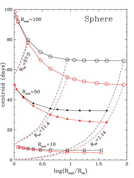
Figure 11: The centroid of the 1-d response function as a function of $R_{\rm out}/R_{\rm in}$ for a spherical geometry and fixed $R_{\rm out}$ of 100 (open circles), 50 (filled triangles) and 10 (open squares) light-days. Also shown (dashed lines) is the centroid of the 1-d response function as a function of $R_{\rm out}/R_{\rm in}$ for fixed $R_{\rm in}$ of 1.14, 11.4 and 57.0 light-days. The colours refer to the slope of the radial power-law emissivity distribution (black: power-law slope $-1$, $\eta(r)=-(\gamma/2)=0.5$, red: power-law slope $-2$, $\eta(r)=-(\gamma/2)=1.0$).

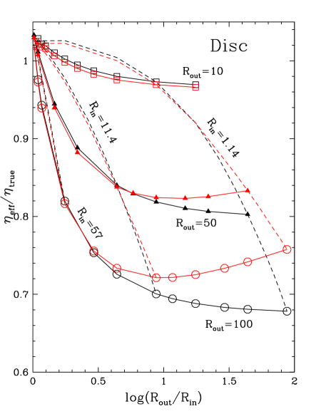
Figure 12: $\eta_{\rm eff}/\eta_{\rm true}$ as a function of $R_{\rm out}/R_{\rm in}$ for a thin-disc geometry and fixed $R_{\rm out}$ of 100 (open circles), 50 (filled triangles) and 10 (open squares) light-days. Also shown (dashed lines), are $\eta_{\rm eff}/\eta_{\rm true}$ as a function of $R_{\rm out}/R_{\rm in}$ for fixed $R_{\rm in}$ of 1.14, 11.4 and 57.0 light-days. The colours refer to the slope of the radial power-law emissivity distribution (black: power-law slope $-1$, $\eta(r)=-(\gamma/2)=0.5$, red: power-law slope $-2$, $\eta(r)=-(\gamma/2)=1.0$).

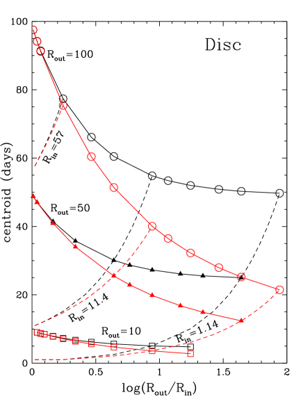
Figure 13: The centroid of the 1-d response function as a function of $R_{\rm out}/R_{\rm in}$ for a disc-shaped BLR geometry and fixed $R_{\rm out}$ of 100 (open circles), 50 (filled triangles) and 10 (open squares) light-days. Also shown (dashed lines) is the centroid of the 1-d response function as a function of $R_{\rm out}/R_{\rm in}$ for fixed $R_{\rm in}$ of 1.14, 11.4 and 57.0 light-days. The colours refer to the slope of the radial power-law emissivity distribution (black: power-law slope $-1$, $\eta(r)=-(\gamma/2)=0.5$, red: power-law slope $-2$, $\eta(r)=-(\gamma/2)=1.0$).

3.3 The role of geometric dilution

As noted above, for BLR geometries with significant spatial extent relative to the characteristic timescale of the driving continuum, we expect a degree of geometric dilution of the measured line responsivity. In previous work, Pogge and Peterson (1992) suggested that a first order correction for the continuum emission-line delays is sufficient to allow an accurate determination of $\eta_{\rm eff}$, showing that data corrected in this fashion displays significantly reduced scatter. Following on from this, Gilbert and Peterson (2003) demonstrated that the $\eta_{\rm eff}$ recovered from the data depends critically upon the fitting process employed, finding values of between 0.53–0.65 for broad H$\beta$ over the full 13 yr ground-based optical monitoring campaign of NGC 5548. They also investigated the dependence of the line responsivity on BLR size, using as an example geometrically-thin spherical BLR geometries represented by top-hat transfer functions. They found that $\eta_{\rm eff}$ varies by only $\approx$5% between transfer functions of half-width 1- and 10 days, so that while the line responsivity decreases as the BLR outer boundary increases, it does so at a very slow rate. Here we expand on this work by examining the role of geometric dilution for spatially extended BLR geometries, and for which a top-hat transfer function is no longer appropriate.

We start by generating spherical, disc, and bowl-shaped BLR geometries, specified by an inner radius $R_{\rm in}$, outer radius $R_{\rm out}$, and for which the emission-line response is taken to be constant across the whole BLR (ie. a locally-linear response approximation ($\eta(r)=constant$ $\forall$ $r$). Initially, both the disc and bowl-shaped BLRs are assumed to be viewed face-on ($i=0$) by an external observer. For non-spherical BLR geometries, other values of observer line of sight inclination only serve to increase the effect of geometric dilution, since for these geometries the spread in delays is orientation dependent and is a maximum when viewed edge-on.

Values of $\eta(r)$ were chosen to encompass the range of values measured in standard photoionisation model calculations of the BLR gas, adopting power-law radial surface line emissivity distributions ($F(r)\propto r^{\gamma}$) with power-law indices of $-1$ and $-2$ (equivalently $\eta(r)=0.5$, 1.0 respectively). For each model BLR, we drive the emission-line response with a continuum light-curve modelled as a damped random walk (Kelly et al. 2009; MacLeod et al. 2010) with a characteristic continuum variability time-scale $T_{\rm char}=40$ days, appropriate for the UV continuum variability observed in the nearby Seyfert 1 galaxy NGC 5548 (Collier and Peterson 2001), and assuming stationary BLR boundaries. This particular choice of $T_{\rm char}$ ensures that the continuum variability timescale is well-matched to the responsivity-weighted size of the BLR over the range in BLR spatial extent explored here. From the input continuum light-curve and resultant broad emission-line light-curve we compute the ratio $\eta_{\rm effl}/\eta_{\rm true}$, where $\eta_{\rm true}$ is the expected responsivity in the absence of geometric dilution, and $\eta_{\rm eff}$ is the measured effective responsivity as determined from the ratio of the fractional variability of the line relative to the fractional variability of the continuum ($F_{\rm var}(\rm line)/F_{\rm var}(\rm cont)$). We have verified using monte carlo simulations that for the duration of the input continuum light-curve used here, the ratio $F_{\rm var}(\rm line)/F_{\rm var}(\rm cont)$ is not sensitive to windowing effects (the dispersion $\sigma$ on $\eta_{\rm eff}$ is less than 0.02 for 1-day sampling over 1000 days duration, see e.g. Figure 7).

3.3.1 Spherical BLR geometries

Figure 10 indicates the ratio $\eta_{\rm eff}/\eta_{\rm true}$ for isotropically emitting BLR clouds occupying a spherical BLR with a range of $R_{\rm out}/R_{\rm in}$, and assuming fixed $R_{\rm out}$ of 100 (open circles), 50 (filled triangles) and 10 (open squares) light-days. Similarly the dashed lines (running from top–bottom) indicate $\eta_{\rm effl}/\eta_{\rm true}$ as a function of $R_{\rm out}/R_{\rm in}$, for fixed $R_{in}$. The colours refer to the power-law index $\gamma$ of the radial surface emissivity distribution (black: $\gamma=-1$, $\eta=0.5$, red: $\gamma=-2$, $\eta=1.0$). In the absence of geometric dilution, we would expect $\eta_{\rm eff}=1.0$ and $0.5$ for radial surface emissivity distributions ($F(r)\propto r^{\gamma}$) with power-law indices $\gamma$ of $-2$ and $-1$ respectively.

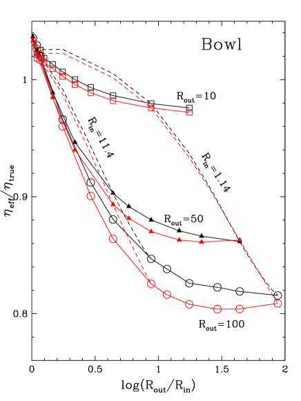
Figure 14: $\eta_{\rm eff}/\eta_{\rm true}$ as a function of $R_{\rm out}/R_{\rm in}$ for a bowl-shaped geometry, and fixed $R_{\rm out}$ of 100 (open circles), 50 (filled triangles) and 10 (open squares) light-days. Also shown (dashed lines), are $\eta_{\rm eff}/\eta_{\rm true}$ as a function of $R_{\rm out}/R_{\rm in}$ for fixed $R_{\rm in}$ of 1.14, 11.4 light-days. The colours refer to the slope of the power-law emissivity distribution (black: power-law slope $-1$, $\eta(r)=-(\gamma/2)=0.5$, red: power-law slope $-2$, $\eta(r)=-(\gamma/2)=1.0$).

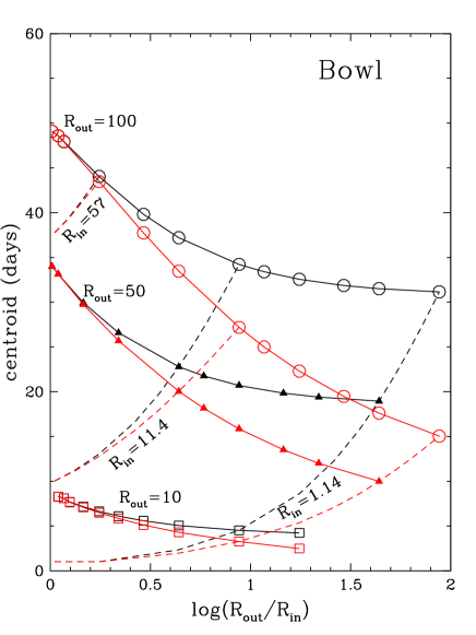
Figure 15: The centroid of the 1-d response function as a function of $R_{\rm out}/R_{\rm in}$ for a bowl-shaped BLR geometry and fixed $R_{\rm out}$ of 100 (open circles), 50 (filled triangles) and 10 (open squares) light-days. Also shown (dashed lines) is the centroid of the 1-d response function as a function of $R_{\rm out}/R_{\rm in}$ for fixed $R_{\rm in}$ of 1.14, 11.4 and 57.0 light-days. The colours refer to the slope of the radial power-law emissivity distribution (black: power-law slope $-1$, $\eta(r)=-(\gamma/2)=0.5$, red: power-law slope $-2$, $\eta(r)=-(\gamma/2)=1.0$).

For a spherical BLR geometry the ratio $\eta_{\rm eff}/\eta_{\rm true}$ remains $\approx$constant for fixed $R_{\rm out}$, for $R_{\rm out}/R_{\rm in}>10$. For geometrically-thin shells, ie. $R_{\rm out}/R_{\rm in}<$ a few, $\eta_{\rm eff}/\eta_{\rm true}$ declines as $R_{\rm in}$ increases. Figure 11, which illustrates the variation in the luminosity-weighted radius (or equivalently the centroid of the 1-d response function, the responsivity-weighted radius) as a function of $R_{\rm out}/R_{\rm in}$, suggests that the origin of this relation is tied to the near constancy of the responsivity-weighted radius (or response function centroid) for large $R_{\rm out}/R_{\rm in}$, and the rapid increase in the luminosity-weighted radius for small $R_{\rm out}/R_{\rm in}$. For our spherical BLR, the emission-line luminosity varies as $dL(r)\propto r^{2+\gamma}dr$, where $\gamma$ is the power-law index of the radial surface emissivity distribution. This yields responsivity-weighted radii of 66 light-days and 49.5 light-days for a BLR spanning $R_{\rm in}=1.14$ and $R_{\rm out}=100$ light-days, for power-law indices $\gamma=-1$ and $\gamma=-2$ respectively.

Similar to Gilbert and Peterson (2003) we find that for thin-shell geometries with outer radii $R_{\rm out}<10$ light-days, $\eta_{\rm eff}$ is close to 90% of the expected value. It is also clear that geometric dilution is larger for flatter emissivity distributions (for a geometrically-thick BLR), and converges for geometrically-thin regions (the separation between the black and red lines declines as $R_{\rm out}/R_{\rm in}\rightarrow 1$). Figure 10 also illustrates that if the location of the BLR inner and outer boundaries are allowed to vary with continuum level, then for a fixed radial surface emissivity distribution, the largest variation in $\eta_{\rm eff}$ results from changes in the location of the BLR outer boundary, for example, follow the dashed vertically running lines in Figure 10.

3.3.2 Disc-shaped BLR geometries

Figure 12 indicates the ratio $\eta_{\rm eff}/\eta_{\rm true}$ as a function of $R_{\rm out}/R_{\rm in}$ for a face-on disc-shaped BLR geometry. In Figure 13 we show the corresponding dependence of the luminosity-weighted radius on $R_{\rm out}/R_{\rm in}$ for this geometry. As for spherical BLR geometries, Figure 12 reveals that for spatially extended regions, ie. $R_{\rm out}/R_{\rm in}>10$, changes in $\eta_{\rm eff}$ due to geometric dilution are dominated by changes in the BLR outer radius. For example, if the BLR outer radius extends to 100 light-days, a factor of 10 change in the inner radius (1.14–11.4 light-days) has little effect on $\eta_{\rm eff}$ since the responsivity-weighted radius increases only very slowly with $R_{\rm in}$. By comparison, for fixed $R_{\rm in}$ a factor of 10 decrease in the outer radius can produce a significant increase in the line responsivity ($\sim 30$% for $R_{\rm out}/R_{\rm in}>10$), owing to the rapid drop in the responsivity-weighted radius with decreasing $R_{\rm out}$ (e.g. Figure 13). However, unlike the spherical BLR geometry, for geometrically-thin discs (or rings), large changes in $\eta_{\rm eff}$ for fixed $R_{out}$ can also arise simply by increasing the inner radius. This difference arises because for a thin shell, the continuum–emission-line delays span the range $0\leq\tau\leq 2R/c$, while for a face-on thin ring of emitting material, the delay is simply $R/c$. The results presented here will change for inclined discs, though not significantly over the expected range in line-of sight inclinations $i\leq 30$ degrees (see e.g. Figure 16 for details). For our disc-shaped BLR, $dL(r)\propto r^{1+\gamma}$. The responsivity-weighted radii for a BLR spanning $R_{\rm in}=1.14$ and $R_{\rm out}=100$ light-days is 49.5 and 22 light-days for power-law indices $\gamma=-1$, and $\gamma=-2$ respectively (e.g. Figure 13). Thus for a disc-shaped BLR, assuming fixed BLR boundaries larger responsivities (e.g. $\eta_{\rm eff}/\eta_{\rm true}>0.9$) requires either a small outer radius ($R_{\rm out}<30$ light-days), or a Ring-like geometry ($R_{\rm out}/R_{\rm in}<$ a few).

3.3.3 Bowl-shaped BLR geometries

Figures 14 and 15 indicate the equivalent relationships for our fiducial bowl-shaped BLR described in §3.1 (see also Goad, Korista and Ruff 2012), this time when viewed face-on ($i=0$). In this model, the BLR bridges the gap between the outer accretion disc and the inner edge of the dusty torus via an effective surface surface the scale height of which increases with increasing radial distance. By placing material at larger radial distances closer to an observer’s line of sight, geometric dilution of the line responsivity is significantly reduced, due to the reduced spread in delays for this geometry, up to a factor 2 for $R_{\rm in}=1.14$ light-days and $R_{\rm out}=100$ light-days (note that for a bowl-like geometry, the gas at larger radii has a smaller surface area for the same radial distance than for a disc), though the general dependence on $R_{\rm out}$ and $R_{\rm in}$ is, by and large, the same as for the thin-disc geometry. The responsivity-weighted radii for our bowl-shaped geometry when viewed face-on and spanning BLR radii $R_{\rm in}=1.14$ – $R_{\rm out}=100$ light-days are 31.1 and 15.0 light-days for power-law indices $\gamma=-1$, and $\gamma=-2$ respectively.

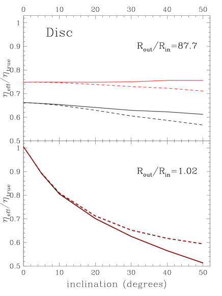
Figure 16: upper panel – $\eta_{\rm eff}/\eta_{\rm true}$ for $R_{\rm out}=100$ light-days, $R_{\rm in}=1.14$ light-days, and power-law emissivity distributions of slope $-1$, $-2$ (equivalently $\eta(r)=0.5$ (black), 1.0 (red) ). Solid lines indicate isotropic emission, dashed lines 100% anisotropy. Lower panel – as above for $R_{\rm in}=98.07$ light-days (ie. $R_{\rm out}/R_{\rm in}\approx 1.0$)

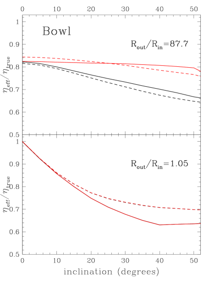
Figure 17: upper panel – $\eta_{\rm eff}/\eta_{\rm true}$ for $R_{\rm out}=100$ light-days, $R_{\rm in}=1.14$ light-days, and power-law emissivity distributions of slope $-1$, $-2$ (equivalently $\eta(r)=0.5$ (black), 1.0 (red) ). Solid lines indicate isotropic emission, dashed lines 100% anisotropy. Lower panel – as above for $R_{\rm in}=98.07$ light-days (ie. $R_{\rm out}/R_{\rm in}\approx 1.0$)

3.4 Anisotropy and inclination

The disc- and bowl-shaped BLR geometries presented in §3.3 assume isotropic cloud emission for a BLR which is viewed face-on (ie. $i=0$). We have also investigated spherical, thin-disc and bowl-shaped geometries in which the line emission from individual BLR clouds is 100% inward toward the ionising continuum source (i.e. fully anisotropic emission), as well as exploring the variation in geometric dilution with line-of-sight inclination. For the anisotropy we here adopt a form which approximates the phases of the moon (e.g. Goad 1995; O’Brien, Goad and Gondhalekar 1994). The effect of anisotropy on the responsivity-weighted radius for both spherical and disc-like BLR geometries has been explored elsewhere (e.g. O’Brien, Goad and Gondhalekar 1994; Goad 1995, PhD thesis).

For geometrically-thick spherical BLR geometries, anisotropy enhances the far side emission relative to the near side emission. The net result is that the response of gas lying closest to the line of sight and which responds on the shortest timescales decreases significantly as the anisotropy increases and consequently the mean response timescale as given by the responsivity-weighted radius (or equivalently the luminosity-weighted radius) increases. In terms of the measured responsivity, the larger responsivity-weighted radius will result in a smaller amplitude emission-line response.

A similar outcome applies to disc-like BLR geometries, though for our adopted form of anisotropy the responsivity-weighted size of the emitting region has a strong inclination dependence, increasing as the inclination increases (note that increased emission-line anisotropy has no effect on the mean response timescale at zero inclination for a disc). Figure 16 (upper panel) illustrates the effect of line anisotropy and inclination on the ratio $\eta_{\rm eff}/\eta_{\rm true}$ for a thin-disc geometry, $R_{\rm out}=100$ light-days, $R_{\rm in}=1.14$ light-days and line-of-sight inclination 0–50 degrees. Solid lines indicate isotropic line emission, dashed lines 100% anisotropy, while colours indicate $\eta=0.5$ (black), $\eta=1.0$ (red). For geometrically-thick ($R_{\rm out}/R_{\rm in}>10$) disc-shaped BLR geometries anisotropy and inclination produce only a modest change in the effective responsivity ($<10$% even at the largest inclination). For a disc-like geometry with purely isotropic emission, inclination increases the spread in the emission-line delays, but the responsivity-weighted size of the BLR remains unchanged. When anisotropy is included, the responsivity-weighted size of a geometrically-thick disc-like BLR increases only very slowly with increasing inclination, because significant front-back asymmetry occurs only for relatively large inclinations.

By contrast, for geometrically-thin disc-like BLR geometries ($R_{\rm out}/R_{\rm in}\sim 1$) the line responsivity $\eta_{\rm eff}$ decreases dramatically with increasing inclination, a purely geometrical effect, while anisotropy tends to increase the responsivity relative to the isotropic case at large inclinations. Though counter intuitive, the latter arises because while the responsivity-weighted size of the BLR increases with increased inclination (in the anisotropic case), the spread in delays is smaller for a thin ring with anisotropic emission relative to the purely isotropic case. For example, if we adopt 30 degrees as a typical inclination, then for a thin ring with $R_{\rm out}/R_{\rm in}\approx 1$, the measured responsivity relative to that found for a face-on thin ring of the same dimensions decreases by $\sim 38$% for isotropic emission, and only $\sim 34$% for fully anisotropic emission (see e.g. Figure 16).

Our fiducial bowl-like BLR geometry exhibits similar behaviour with anisotropy and inclination to that of a disc-like BLR, but with some subtle geometry related differences (Figure 17). The bowl is not front-back symmetric, thus even in the isotropic emission case, the responsivity-weighted radius will increase with increasing inclination, though only weakly. However, at inclinations greater than 45 degrees self-occultation occurs and the delay increases significantly as substantial material lying close to the line of sight is obscured from view (see e.g. Figure 1 of Goad, Korista and Ruff 2012). When anisotropy is included, initially the mean delay is reduced as emission from gas lying on the steep sides of the bowl is reduced, removing contributions of gas at large delays. As the bowl is inclined further, the responsivity-weighted radius increases. When considering only the extreme outer rim of the bowl, the observed behaviour is similar to that for a thin ring, $\eta_{\rm eff}$ decreases sharply with increased inclination. However, for the bowl the responsivity stabilises for inclinations above $\approx 20$ degrees.

4 Discussion : a Breathing BLR

The 13 yr ground-based spectroscopic monitoring campaign of the nearby Seyfert 1 galaxy NGC 5548 indicates that the broad H$\beta$ line EW is time-variable, changing by more than a factor of 2 on timescales less than a typical observing season ($\approx$ 200 days) (lower panel of Figure 1). Indeed the measured broad H$\beta$ line EW, which is a measure of the continuum re-processing efficiency of the line-emitting gas for this line, is found to be inversely correlated with continuum level, such that the largest EWs are found during low continuum states. The line EW is related to the effective emission-line responsivity $\eta_{\rm eff}$ via equation 2, which indicates that a time-variable line EW is to be expected if $\eta_{\rm eff}\neq 1$. If even after accounting for the effects of geometric dilution $\eta_{\rm eff}\approx 1$, then following equation 2 the re-processing efficiency for a particular line will remain approximately constant (ie. EW(line)$\approx$ constant, ie. no intrinsic Baldwin effect). Since EW(H$\beta$) is found to be inversely correlated with continuum level in NGC 5548 (an intrinsic Baldwin effect for H$\beta$), the effective responsivity must be less than $1$ for this line.

We note here that the inverse correlation found between ionising continuum flux and the emission-line re-processing efficiency is a key prediction (and a major success) of photoionisation model calculations (e.g. Korista and Goad 2004, their Figures 3 and 4). Specifically, Korista and Goad (2004) found that for the hydrogen and helium recombination lines the local (in-situ) emission-line responsivity $\eta$ increases toward lower hydrogen ionising continuum fluxes independent of any assumed geometry. Thus in the absence of those effects which act to reduce the emission-line responsivity (e.g. geometric dilution), photoionisation models predict that locally the emission-line responsivity $\eta$ will increase as the ionising continuum flux decreases (ie. $\eta=\eta(L_{\rm cont}(t))$, e.g. Figure 2, cf. solid and dashed black lines).

A key goal of the present work was to determine how the properties of the driving continuum light-curve (ie. its amplitude and characteristic timescale), observational bias (e.g. light-curve duration and sampling pattern) and choice of BLR geometry, contribute to the measured emission-line responsivity $\eta_{\rm eff}$. To isolate these effects from those caused by changes in the local gas physics arising from ionising continuum flux variations, we have assumed a radial surface emissivity distribution which is a power-law in radius and a locally-linear response approximation for a BLR with fixed inner and outer boundaries. For a power-law radial surface emissivity distribution, $F(r)\propto r^{\gamma}$, $\eta(r)=-(\gamma/2)=constant\,,\forall r$. While locally the radial surface emissivity increases with continuum level, it does so by the same amount everywhere. Thus the radial dependence, if not the absolute value of the radial surface emissivity distribution, is the same and thus the instantaneous responsivity-weighted radius is constant in time. Since both the radial line responsivity and responsivity-weighted radius are constant $\forall r,t$, such a broad-line region cannot breathe (the characteristic emission-line response amplitude and delay are constant in time). Thus for these models we do not expect to find a correlation between BLR size and continuum state nor an inverse correlation between the emission-line responsivity $\eta_{\rm eff}$ and continuum state.

Photoionisation model calculations by Goad, O’Brien and Gondhalekar (1993), and Korista and Goad (2004), indicate that power-law radial surface emissivity distributions are generally a poor approximation to the predicted behaviour of the majority of the strong broad UV and optical emission-lines. In Figure 2 we illustrate the radial surface emissivity distribution $F(r)$ (upper panel) and radial line responsivity $\eta(r)$ (lower panel) for broad H$\beta$ as determined for an LOC model of the BLR in NGC 5548 (Korista and Goad 2004).

For broad H$\beta$ the radial surface emissivity distribution is best represented by a broken power-law with a power-law index $\gamma\approx-0.7$ for radii less than $\approx 25$ light-days and breaks towards values in $\gamma$ steeper than $\approx-2$ for radii greater than $\approx 160$ light-days (as indicated by the red line in the upper panel of Figure 2). The corresponding values in the radial responsivity distribution spans $\eta(r)\approx 0.35$ in the inner BLR to values of $\eta(r)\approx 1$ or more beyond the confines of our fiducial BLR outer boundary.

Because in general, emission-line emissivities are not strictly power-laws, $\eta(r)\neq constant$, such a BLR will breathe even if the boundaries of the BLR remain fixed at their starting values (Korista and Goad 2004). Consequently the responsivity-weighted radius (or equivalently the luminosity-weighted radius as measured from the centroid of the CCF) will vary with continuum state due to changes in the relative radial surface emissivity distribution with continuum flux within the confines of those fixed boundaries. Figure 2 illustrates the H$\beta$ radial surface emissivity distributions and their respective radial responsivity distributions corresponding to small continuum variations about low- and high-continuum states (dashed and solid black lines respectively). These states were chosen to match two historical extrema in the UV continuum flux of NGC 5548 and correspond to a peak-peak variation of $\approx 8.2$ (or equivalently $0.5\times\log 8.2=0.457$ in $\log r$). Compare their behaviour to that of a simple power-law radial emissivity distribution (as indicated by the green lines in Figure 2) for which the luminosity-weighted radius and emission-line responsivity are invariant.

For most lines, including H$\beta$, the local radial responsivity distribution $\eta(r)$ generally decreases with increased ionising continuum flux, which when integrated over the whole BLR results in a reduction in the emission-line responsivity and an increase in the delay (e.g. Korista and Goad 2004, their Figure 3; Goad, Korista and Ruff 2012, their Figure 9). This finding is independent of those effects discussed in §3 (for example, $T_{\rm char}$, $T_{\rm dur}$ and BLR geometry) which when folded in, act to further reduce the measured emission-line responsivity. Korista and Goad (2004) found low- and high-continuum state responsivities for H$\beta$ spanning the range 0.54–0.77 (columns 3 and 4 of their Table 1) in the absence of those effects which act to reduce the emission-line responsivity. The measured range in $\eta_{\rm eff}$ when referenced to the amplitude of the UV continuum variations is significantly larger, $0.33<\eta_{\rm eff}<0.84$, and is inversely correlated with continuum level (Goad, Korista and Knigge 2004; Bentz et al. 2009).

Figures 12 and 14 show that for steep radial surface emissivity distributions, it is difficult for geometric dilution alone to reduce $\eta_{\rm eff}$ to values as low as $\approx 0.3$. With our adopted value of $T_{\rm char}=40$ days the emission-line response is already significantly geometrically diluted for the geometries presented here. By implication, the radial surface emissivity distribution for H$\beta$ is unlikely to be steep as $\gamma=-2$.

The measured upper bound of $\eta_{\rm eff}=0.84$ is larger than the upper bound quoted in Korista and Goad (2004). This is particularly intriguing, since we have already shown that $T_{\rm char}$, $T_{\rm dur}$ and BLR geometry, generally act to dilute the emission-line responsivity. Adopting a smaller outer boundary for our model BLR cannot help here because the in-situ responsivity is small at small BLR radii for broad H$\beta$. One possible explanation is that the amplitude of the driving ionising continuum is significantly larger than that used here, and subsequently the measured range in emission-line responsivity when integrated over the whole BLR will be larger between the high- and low- continuum states than considered in Korista and Goad (2004). For a BLR of fixed radial extent we can enhance the radial responsivity at smaller BLR radii by adopting a smaller continuum normalisation. This will consequently reduce the responsivity-weighted radius. When reverberation effects are then taken into consideration, this will produce a more coherent emission-line response. A smaller continuum normalisation may also result in a smaller BLR outer boundary.

Because of geometric dilution, spatially extended BLRs will exhibit a large effective responsivity in H$\beta$ only if the intrinsic (local gas) responsivities are significantly larger than those shown here. Such large intrinsic responsivities require low incident ionising photon fluxes, which as shown in Figure 2 lie beyond the outer boundary of our model geometry. Alternatively, larger $\eta_{\rm eff}$ for H$\beta$ may also be obtained if the radial surface emissivity curve is moderately steeper than that shown here. This can be achieved for example by including gas at densities $>10^{12}$ cm^-3, or if locally the line emitting gas experiences significant extra-thermal line broadening (e.g. Bottorff et al. 2000).

Finally, we haven’t yet touched upon the possibility that the location of the BLR inner and outer boundaries may also vary in response to continuum variations. Figures 10–15 suggest that relaxing the assumption of fixed BLR boundaries will allow large changes in the emission-line responsivity and delay to occur. We defer investigation of the effects of a radially-dependent and continuum-level dependent emission-line responsivity (breathing) and the possible time-variable location of the BLR inner and outer boundaries in response to continuum variations to paper ii.

5 Conclusions

The measured amplitude and delay of the emission-line response to continuum variations is determined by the local gas physics, the BLR geometry and the characteristics of the driving ionising continuum ($T_{\rm char}$, $T_{\rm dur}$ and $\Delta t$). The role of the local gas physics in determining the emission-line responsivity has been explored in Korista and Goad (2004). Here, we focus on the remaining aforementioned effects which act to modify the local emission-line responsivity.

We have demonstrated two independent methods for the determination of the effective emission-line responsivity $\eta_{\rm eff}$ each with similar accuracy. The standard approach using the logarithmic slope of the relation between the continuum–emission-line fluxes $d\log f_{\rm line}/d\log f_{\rm cont}$, is more difficult to determine, requiring a correction for the continuum–emission-line delay and normally involves interpolating on one of the light-curves. The second method is far simpler to implement and requires only the determination of the ratio of the fractional variance of the line to the fractional variance of the continuum $F_{\rm var}$(line)/$F_{\rm var}$(cont). Indeed for the latter, continuum and emission-line data need not be contemporaneous, though the dependence of responsivity on continuum level is lost (the latter may in part be recovered by investigating the variability of the continuum and emission-line light-curves as a function of continuum state). Both methods require a suitable correction for contaminating non-variable components in the line (from contaminating narrow mission-lines) and continuum (from the host galaxy).

Importantly, our simulations indicate that light-curve duration plays an important role in the determination of the effective emission-line responsivity $\eta_{\rm eff}$, and a similar effect is found for the continuum emission-line delay. For short observing campaigns the measured value of $\eta_{\rm eff}$ is biased towards smaller values with a larger intrinsic scatter. Reduced sampling rates do not affect the measured value of $\eta_{\rm eff}$, though the error on a single estimate increases as the sampling rate decreases. This suggests that measuring the “true” responsivity of a given emission-line requires light-curves of sufficient duration, typically longer than the autocorrelation function of the continuum light-curve. While noteworthy, the observational bias toward smaller responsivity introduced by a shorter duration campaigns can not explain the observed inverse correlation between $\eta_{\rm eff}$ and continuum level. Simulations such as these may be used to inform the design of future intensive reverberation mapping campaigns.

Contrary to previous work, our simulations indicate that geometric dilution may play a significant role in reducing the effective emission-line responsivity. For a BLR of fixed spatial extent, and a characteristic continuum variability timescale $T_{\rm char}$ which is less than the maximum delay for a particular line $\tau_{\rm max}$(line), for a given BLR geometry and observer line-of-sight orientation, the effective emission-line responsivity $\eta_{\rm eff}$, emission-line delay and the maximum of the continuum–emission-line cross-correlation coefficient are strongly correlated (Figure 9, panels (ii) and (v)). For example, our simulations suggest that for our fiducial BLR model, $\eta_{\rm eff}$ decreases significantly for $T_{\rm char}\leq 100$ days, the maximum delay at the outer radius for our fiducial BLR geometry when observed at a line of sight inclination of 30 degrees. This suggests that for a given BLR geometry, the characteristic continuum variability timescale, $T_{\rm char}$, is a key quantity in the determination of the measured emission-line responsivity and delay. Importantly, if $T_{\rm char}\geq\tau_{\rm max}$(line) geometric dilution is minimised and the measured responsivity and delay may be considered as representative of the underlying gas responsivity and mean response timescale. Conversely, if $T_{\rm char}<\tau_{\rm max}$(line), geometric dilution can act to significantly reduce the measured emission-line responsivity and delay.

Changes in the short timescale variability amplitude of the continuum light-curve appear to be less important in the determination of $\eta_{\rm eff}$ and delay, over the range in variability amplitude expected for the driving continuum light-curve. Significantly, if for a fixed continuum luminosity, the characteristic continuum variability timescale $T_{\rm char}$ and BLR ’size’ varies among the AGN population, then geometric dilution in individual sources will introduce scatter into the well-known BLR radius–luminosity relation.

Following on from the work of Gilbert and Peterson (2003), we have explored the effect of geometric dilution on emission-line responsivity for spherical, disc and bowl-shaped BLR geometries, spanning a range of BLR sizes (both geometrically-thick and geometrically-thin) using a fixed characteristic timescale and amplitude for the driving continuum light-curve. In the majority of cases the measured responsivities are found to be largest for smaller (more compact) BLRs (Figures 10, 12, and 14). For disc- and bowl-shaped BLR geometries, the largest responsivities are found for geometrically-thin BLRs, neglecting the effects of inclination. For geometrically-thick BLRs, the measured responsivity $\eta_{\rm eff}$ is strongly correlated with the characteristic size of the line-emitting region (Figures 11, 13, and 15). Significantly, Figures 10, 12, and 14 suggest that large changes in an emission-line’s responsivity may be realised, if we relax the assumption of fixed BLR boundaries. We explore this further in paper ii.

6 Acknowledgements

We would like to thank the referee for some helpful suggestions which have helped to improve the clarity of the work presented here. We would also like to thank Anna Pancoast for a very careful reading of the original manuscript which helped to improve the clarity of the work presented here. Mike Goad would also like to thank Kirk and Angela Korista and Western Michigan University for their generous hospitality during the early stages of this work.

7 References

Baldwin, J. Ferland, G., Korista, K., and Verner, D., 1995, ApJ 455, 119.

Bentz, M.C., Walsh, J.L., Barth, A.J., Baliber, N., Bennert, V.N. et al., 2009, ApJ 705, 199.

Bentz, M.C., Peterson, B.M., Pogge, R.W. et al., 2006, ApJ 644, 133.

Bottorff, M., Ferland, G., Baldwin, J. and Korista, K. 2000, ApJ 542, 644.

Cackett, E.M. and Horne, K., 2006, MNRAS 365, 1180.

Clavel, J. Reichert, G.A. Alloin, D. et al., 1991, ApJ 366, 64.

Collier, S. and Peterson, B.M., 2001, ApJ 555, 775.

Collier, S.J., Peterson, B.M. and Horne, K., 2001, BAAS, vol 333, p896.

Czerny, B., Doroshenko, V. T., Nikołajuk, M., et al., 2003, MNRAS, 342, 1222

Denney, K.D., Peterson, B.M., Dietrich, M., Vestergaard, M. and Bentz, M.C., 2009, ApJ 692, 246.

Ferland, G.J., Peterson, B.M., Horne, K. Welsh, W.F., Nahar, S.N., 1992, ApJ 387, 95.

Gaskell, C.M. and Peterson, B.M., 1987, ApJS 65, 1.

Gilbert, K.M. and Peterson, B.M., 2003, ApJ 587, 123.

Goad, M. R.; Korista, K. T. and Ruff, A.J., 2012, MNRAS 426, 3086.

Goad, M. R.; Korista, K. T.; Knigge, C., 2004, MNRAS 352, 277.

Goad, M.R. and Wanders, I., 1996, ApJ 469, 113.

Goad, M.R., 1995, PhD thesis, University College London.

Goad, M.R., O’Brien, P.T. and Gondhalekar, P.M., 1993, MNRAS 263, 149.

Han, X.-H., Wang, J., Wei, J.-Y., Yang, D.-W. and Hou, J.-L., 2011, Science China, Physics Mechanics and Astronomy, 54, 346.

Horne, K., Welsh, W.F. and Peterson, B.M. 1991, ApJ 367, L5.

Horne, K., Peterson, B.M., Collier, S.J. and Netzer, H., 2002, astro-ph 1182.

Horne, K., Korista, K.T. and Goad, M.R., 2003, MNRAS 339, 367.

Kong, M.-Z., Wu, X.-B, Wang, R. Liu, F.K. and Han, J.L., 2006, A&A 456, 473.

Kelly, B.C., and Bechtold, J., 2007 ApJS 168, 1.

Kelly, B.C., Bechtold, J., Siemiginowska, A., 2009, ApJ 698, 895.

Koratkar, A.P. and Gaskell, C.M. ApJS 74, 719.

Korista, K.T., Alloin, D., Barr, P. et al., 1995, ApJS 97, 258.

Korista, K.T. and Goad, M.R., 2000, ApJ 536, 284.

Korista, K.T. and Goad, M.R., 2001, ApJ 553, 695.

Korista, K.T. and Goad, M.R., 2004, ApJ 606, 749.

Kozlowski, S. Kochanek, C.S., Udalski, A. et al., 2010, ApJ 708, 927.

Krause, M., Schartmann, M. and Burkert, A., 2012, MNRAS 425, 3172.

Krolik, J.H., Horne, K., Kallman, T.R. et al., 1991, ApJ 371, 541.

MacLeod, C.L., Ivezić, Z., Kochanek,C.S. et al., 2010, ApJ 721, 1014.

Maoz, D., Netzer, H., Peterson, B.M., Bechtold, J., Bertram, R. et al., 1993, ApJ 40, 576.

Maoz, D. 1992 In “Physics of Active Galactic Nuclei.” Editors, W.J. Duschl, S.J. Wagner, P.214, 1992

Netzer, H. and Maoz, D., 1990, ApJ, 365, 5.

Netzer, H. and Laor, A., 1993, ApJ 404, 51.

O’Brien, P.T. Goad, M.R. and Gondhalekar, P.M., 1994, MNRAS 268, 845.

O’Brien, P.T., Goad, M.R. and Gondhalekar, P.M., 1995, MNRAS, 275, 1125.

Penston, M. V. 1991, in “Variability of Active Galactic Nuclei” eds, Miller H.R., Wiita, P.J. Cambridge University Press, p43.

Peterson, B. M., Berlind, P., Bertram, R., Bischoff, K., Bochkarev, N. G et al., 2002, ApJ 581, 197.

Peterson, B.M., Alloin, D., Axon, D., Balonek, T.J., Betram, R. et al., 1992, ApJ 392, 470.

Peterson, B. M., Berlind, P., Bertram, R., Bochkarev, N. G., Bond, D., et al., 1994, ApJ 425, 622.

Peterson, B.M., Denney, K.D., De Rosa, G., Grier, C.J., Pogge, R.W. et al., 2013, ApJ 779, 109.

Pogge, R.W. and Peterson, B.M., 1992, AJ, 103, 1084.

Pérez, E., Robinson, A., and de La Fuente, L., 1992a, MNRAS 255, 502.

Pérez, E., Robinson, A., and de La Fuente, L., 1992b, MNRAS 256, 103.

Press, W.H., Teukolsky, S.A., Saul, A., Vetterling, W.T. and Flannery, P., 1992. Cambridge: University Press, c1992, 2nd ed.

Robinson, A. and Pérez, E., 1990. MNRAS, 244, 138.

Runnoe, J.C., Brotherton, M.S., Shang, Z., Wills, B.J. and DiPompeo, M.A., 2013, MNRAS 429, 135.

Shen, Y. Greene, J.E. Strauss, M.A., Richards, G.T. and Schneider, D.P., 2008, ApJ 680, 196.

Shen, Y. and Kelly, B.C. 2010, ApJ 713, 41.

Suganuma, M., Yoshii, Y., Kobayashi, Y. et al., 2006, ApJ 639, 46.

Uttley, P., McHardy, I.M., and Vaughan, S., 2005, MNRAS 359, 345.

Vestergaard, M. and Peterson, B.M., 2005, ApJ 625, 688.

Welsh, W.F., 1999, PASP 111, 1347.

Welsh, W.F. and Horne, K., 1991, ApJ 379, 586.

Zu, Y., Kochanek, C.S., Peterson, B.M., 2011, ApJ 735, 80.