Critical behavior of the random-field Ising model with long-range interactions in one dimension

Abstract

We study the critical behavior of the one-dimensional random field Ising model (RFIM) with long-range interactions ($\propto r^{-(d+\sigma)}$) by the nonperturbative functional renormalization group. We find two distinct regimes of critical behavior as a function of $\sigma$, separated by a critical value $\sigma_{c}$. What distinguishes these two regimes is the presence or not of a cusp-like nonanalyticity in the functional dependence of the renormalized cumulants of the random field at the fixed point. This change of behavior can be associated to the characteristics of the large-scale avalanches present in the system at zero temperature. We propose ways to check these predictions through lattice simulations. We also discuss the difference with the RFIM on the Dyson hierarchical lattice.

I Introduction

The random field Ising model (RFIM) has been the focus of intense investigation as one of the paradigms of criticality in the presence of quenched disorder.imry-ma75 ; nattermann98 It has found application in physics and physical chemistry as well as in interdisciplinary fields such as biophysics, socio- and econo-physics. The model displays a phase transition, a paramagnetic-to-ferromagnetic one in the language of magnetic systems, and the long-distance physics is dominated by disorder-induced sample-to-sample fluctuations rather than by thermal fluctuations. In the renormalization-group (RG) sense, the critical behavior is then controlled by a fixed point at zero temperature and its universal properties can also be studied by investigating the model at zero temperature as a function of disorder strength.

One of the central issues arising in the RFIM was the so-called dimensional-reduction property, according to which the critical behavior of the random system is the same as that of the pure system in a dimension reduced by 2. This was found at all orders of perturbation theorygrin_76 ; young_77 and was related to the presence of an underlying supersymmetry.parisi_79 . The property fails in low dimension, in particular in $d=3$ imbrie_84 ; brich_kup_87 and a resolution of the problem was found within the framework of the nonperturbative functional RG (NP-FRG).tarjus04 ; tissier06 ; tissier11 Within the NP-FRG, the breakdown of dimensional reduction and the associated spontaneous breaking of the underlying supersymmetry are attributed to the appearance of a strong enough nonanalytic dependence, a “cusp”, in the dimensionless renormalized cumulants of the random field at the fixed point.

What appears specific to random-field systems among the disordered models whose long-distance behavior is controlled by a zero-temperature fixed point for which perturbation theory predicts the $d\rightarrow d-2$ dimensional-reduction property, as, e.g., interfaces in a random environment,fisherFRG ; FRGledoussal-chauve ; FRGledoussal-wiese is the existence of two distinct regimes of the critical behavior separated by a nontrivial value of the dimension,tarjus04 ; tissier11 or of the number of components in the O(N) model,tissier06 or else of the power-law exponent of the interactions for the long-range models.bacz_LR3d This is actually what requires a RG treatment that should be not only functional but also nonperturbative (hence, the NP-FRG).

It was shown in Ref. [tarj_avlnch, ] that these two regimes are related to the large-scale properties of the “avalanches”, which are collective phenomena present at zero temperature. In equilibrium, such “static” avalanches describe the discontinuous change in the ground state of the system at values of the external source that are sample-dependent. At the critical point, the avalanches always take place on all scales. However, whether or not they induce a “cusp” in the dimensionless renormalized cumulants of the random field at the fixed point depends on their scaling properties, and more specifically on the fractal dimension $d_{f}$ of the largest typical avalanches at criticality compared to the scaling dimension of the total magnetization.tarj_avlnch

In the short-range RFIM the change of critical behavior appears in a large, noninteger dimension $d\approx 5.1$,tarjus04 ; tissier06 ; tissier11 which is therefore not accessible to lattice simulations. The interest of introducing long-range interactions is that this reduces the dimensions where a phase transition can be observed and provides an additional control parameter with the power-law exponent governing the spatial decay of the interactions. In Ref. [bacz_LR3d, ], a $3$-dimensional RFIM with both long-range interactions and long-range correlations of the random field was studied. The long-distance decays were chosen in such a way that the supersymmetry which is responsible for dimensional reduction is still present in the theory. It was then shown that the spontaneous breaking of supersymmetry and the associated breakdown of dimensional reduction do take place in this $3-d$ model and that two regimes of critical behavior are present and separated by a nontrivial value of the power-law exponents.bacz_LR3d

In this work, we further reduce the dimension of interest to $d=1$ by considering the RFIM with long-range interactions but short-range correlations of the disorder. This model should be even more accessible to lattice simulations (see for instance the recent studies in Refs. [leuzzi, ; dewenter, ]). This should allow an independent check of the scenario derived from the NP-FRG.

In the model the interactions decay with distance as $r^{-(d+\sigma)}$ with $\sigma>0$. In some sense, varying $\sigma$ has a similar effect to that of changing the spatial dimension in the short-range case. For $\sigma\leq\sigma_{G}=1/3$, the critical behavior is governed by a Gaussian fixed point and the exponents are therefore the classical (mean-field) ones in the presence of long-range interactions: $\sigma_{G}$ is the analog of an upper critical dimension. On the other hand, heuristic arguments predict that no phase transition takes place for $\sigma\geq\sigma_{M}=1/2$:Bray ; leuzzi $\sigma_{M}$ is then the analog of an upper critical dimension. The interesting range is therefore $1/3\leq\sigma<1/2$. (Rigorous results show the existence of a phase transition for $2-(\ln 3/\ln 2)\approx 0.4150\cdots<\sigma<1/2$cassandro09 and it is even more likely that a transition exists for smaller values of $\sigma$.)

We investigate through the NP-FRG whether this $1$-dimensional long-range RFIM displays, as the other random-field models studied so far, two regimes of critical behavior separated by a nontrivial value, here of $\sigma$. In this model, there is of course no $d\rightarrow d-2$ dimensional-reduction property and no associated supersymmetry. The two regimes should therefore be characterized by the presence or not of a “cusp” in the functional dependence of the (dimensionless) renormalized cumulants of the random field at the fixed point.

We do find two distinct regimes separated by the critical value $\sigma_{c}\approx 0.379$: a “cuspless” one below $\sigma_{c}$ and a “cuspy” one above. We calculate the critical exponents, which do not show any significant change of behavior around $\sigma_{c}$. More significant is the variation of the fractal dimension $d_{f}$ of the largest critical avalanches, and we discuss the way to assess the validity of the predictions in computer simulations. We also discuss the RFIM on a Dyson hierarchical model with the same parameter $\sigma$. Based on the results given in the literaturerodgers-bray ; monthus11 , we conclude that this model displays a unique “cuspless” regime over the whole range of $\sigma$, with the avalanche-induced cuspy contributions being subdominant at the fixed point.

II Model and NP-FRG formalism

We study the one-dimensional random-field Ising model with power-law decaying long-range ferromagnetic interactions.grin_76 ; Bray It is described by the following Hamiltonian:

$$\begin{split}H=-\sum_{i,j}J_{ij}s_{i}s_{j}-\sum_{i}h_{i}s_{i}\end{split}$$ (1)

where $s_{i}=\pm 1$ are Ising spins placed on the vertices of a lattice, with a ferromagnetic pairwise interaction

$$J_{ij}\propto|x_{i}-x_{j}|^{-(d+\sigma)}$$ (2)

at long distance. The exponent $\sigma>0$ characterizes the long-range power-law decay of the interaction and $d$ is the spatial dimensionality. In the present case $d=1$. The disorder is introduced by the random fields $h_{i}$, which are independently distributed with a Gaussian distribution of width $\Delta_{B}$ around a zero mean:

$$P(h_{i})=\frac{1}{\sqrt{2\pi\Delta_{B}^{2}}}e^{-\frac{h_{i}^{2}}{2\Delta_{B}}}\,.$$ (3)

To make use of the NP-FRG formalism and investigate the long-distance properties of the model near its critical point, it is more convenient reformulate the model in the field-theory setting. By using standard manipulations, the Hamiltonian in Eq. (1) is replaced by the “bare action” for a scalar field $\varphi$:

$$\begin{split}&S[\varphi;h]=S_{B}[\varphi]-\int_{x}h(x)\varphi(x)\\ &S_{B}=\int_{x}\big{[}\frac{r}{2}\varphi(x)^{2}+\frac{u}{4!}\varphi(x)^{4}\big{]}+\frac{1}{2}\int_{x,y}\mathcal{J}(|x-y|)\varphi(x)\varphi(y)\end{split}$$ (4)

where $\int_{x}=\int d^{d}x$ and $h(x)$ is the continuous version of the random magnetic field with $\overline{h(x)}=0$ and $\overline{h(x)h(y)}=\Delta_{B}\delta^{(d)}(x-y)$ (where as usual the overline denotes the average over the quenched disorder). The interaction $\mathcal{J}(|x|)$ goes as $|x|^{-(d+\sigma)}$ at large distance and, accordingly, its Fourier transform behaves as

$$\mathcal{J}(p)=\mathcal{J}|p|^{\sigma}+{\rm O}(p^{2})$$ (5)

when $p\rightarrow 0$.

From here, the NP-FRG equations can be derived along two alternative routes. In the first one, the system is considered directly at zero temperature and one builds a superfield formalism that can account for the fact that the equilibrium properties are given by the ground state of the model.tissier11 ; bacz_LR3d In the second one, the system is considered at finite temperature and one works with the Boltzmann weight.tarjus04 ; tissier06 The main advantage of the former is that it makes explicit the underlying supersymmetry that is responsible for the $d\rightarrow d-2$ dimensional-reduction property and allows one to study its spontaneous breaking along the NP-FRG flow. The latter one is however quite simpler to present and in the following we will follow this route. We stress that the two derivations lead to the same exact NP-FRG equations for the zero-temperature fixed point controlling the critical behavior of the RFIM.

Due to the presence of quenched disorder the generating functional of the (connected) correlation functions, $\mathcal{W}_{h}[J]=\ln\int\mathcal{D}\varphi\,{\rm exp}(-S[\varphi;h]+\int_{x}J(x)\varphi(x))$, is random and can then be characterized by its cumulants. The latter are conveniently studied by considering copies or replicas of the system (see e.g. Refs. [tarjus04, ; tissier11, ]) which, differently from the standard replica trick,Par_book are each coupled to a distinct external source. After averaging over the disorder, the resulting “multicopy” generating functional $W[\{J_{a}\}]=\ln\overline{\prod_{a}{\rm exp}(\mathcal{W}_{h}[J_{a}])}$ is given by

$$\begin{split}&e^{W[\{J_{a}\}]}=\int\prod_{a}\mathcal{D}\varphi_{a}{\rm exp}\Big{\{}\sum_{a}\Big{(}-S_{B}[\varphi_{a}]\\ &+\int_{x}J_{a}(x)\varphi_{a}(x)\Big{)}-\Delta_{B}\sum_{a,b}\int_{x}\varphi_{a}(x)\varphi_{b}(x)\Big{\}}\,.\end{split}$$ (6)

The cumulants are generated by expanding in increasing number of unrestricted (or free) sums over replicas:

$$W[\{J_{a}\}]=\sum_{a}W_{1}[J_{a}]+\frac{1}{2}\sum_{a,b}W_{2}[J_{a},J_{b}]+\cdots,$$ (7)

where $W_{k1}[J_{a}]=\overline{\mathcal{W}_{h,k}[J_{a}]}$ is the first cumulant, $W_{k2}[J_{a},J_{b}]=\overline{\mathcal{W}_{h,k}[J_{a}]\mathcal{W}_{h,k}[J_{b}]}|_{c}$ the second cumulant, etc.

The formulation of the NP-FRG proceeds by modifying the partition function in Eq. (LABEL:bare_Zn) with the introduction of an “infrared regulator” that suppresses the integration over the modes with momentum less than some cutoff $k$ and takes the form of a generalized “mass” (quadratic) term added to the bare action:Ber02

$$\begin{split}\Delta S_{k}[\{\varphi_{a}\}]=\frac{1}{2}\sum_{a,b}\int_{x,y}\varphi_{a}(x)\mathcal{R}_{k,ab}(|x-y|)\varphi_{b}(y)\,,\end{split}$$ (8)

where $\mathcal{R}_{k,ab}=\widehat{R}_{k}\delta_{ab}+\widetilde{R}_{k}$ with $\widehat{R}_{k}$ and $\widetilde{R}_{k}$ two functions enforcing an infrared cutoff on the fluctuations.tissier11 Through this procedure, one defines the generating functional of the (connected) correlation functions at scale $k$, $W_{k}[\{J_{a}\}]$.

In the NP-FRG approach, the central quantity is the “effective average action” $\Gamma_{k}$, which is the generating functional of the one-particle irreducible (1PI) correlation functions or vertices and is obtained from $W_{k}[\{J_{a}\}]$ through a (modified) Legendre transform:

$$\Gamma_{k}[\{\phi_{a}\}]+\Delta S_{k}[\{\phi_{a}\}]=-W_{k}[\{J_{a}\}]+\sum_{a}\int_{x}J_{a}(x)\phi_{a}(x),$$ (9)

where the field $\phi_{a}=\delta W_{k}/\delta J_{a}(x)$ is the average of the physical field in copy $a$.

Similarly to $W_{k}[\{J_{a}\}]$, $\Gamma_{k}[\{\phi_{a}\}]$ can be expanded in an increasing number of free replica sums,

$$\Gamma_{k}[\{\phi_{a}\}]=\sum_{a}\Gamma_{k1}[\phi_{a}]-\frac{1}{2}\sum_{a,b}\Gamma_{k2}[\phi_{a},\phi_{b}]+\cdots\,,$$ (10)

where the $\Gamma_{kp}$’s are essentially the cumulants of the renormalized disorder.tarjus04 ; tissier11

The $k$ dependence of the effective average action is governed by an exact renormalization-group (RG) equation:wetterich93 ; Ber02

$$\partial_{t}\Gamma_{k}[\{\phi_{a}\}]=\frac{1}{2}{\rm Tr}\widetilde{\partial}_{t}\ln(\Gamma^{(2)}_{k}[\{\phi_{a}\}]+\mathcal{R}_{k})\,,$$ (11)

where $t=\ln(k/\Lambda)$, $\widetilde{\partial}_{t}$ is a symbolic notation indicating a derivative acting only on the $k$ dependence of the cutoff functions (i.e., $\widetilde{\partial}_{t}\equiv\partial_{t}\widehat{R}_{k}\,\delta/\delta\widehat{R}_{k}+\partial_{t}\widetilde{R}_{k}\,\delta/\delta\widetilde{R}_{k}$), and $\Gamma^{(2)}_{k}$ is the second functional derivative of the effective average action with respect to the replica fields. (Generically, superscripts indicate functional differentiation with respect to the field arguments.) Finally, the trace involves summing over copy indices and integrating over spatial coordinates.

The initial condition of the RG flow when $k=\Lambda$, the microscopic scale (e.g. the inverse of the lattice spacing), is provided by the bare action and when $k\rightarrow 0$ one recovers the effective action of the full theory with all fluctuations accounted for.

After expanding both sides of Eq. (11) in an increasing number of free replica sums, one obtains a hierarchy of exact RG flow equations for the cumulants of the renormalized disorder. For instance, the equations for first two cumulants read

$$\begin{split}&\partial_{t}\Gamma_{k1}[\phi_{a}]=\\ &-\frac{1}{2}\tilde{\partial}_{t}{\rm tr}\Big{\{}\ln\widehat{G}_{k}[\phi_{a}]+\widehat{G}_{k}[\phi_{a}]\Big{(}\Gamma_{k2}^{(11)}[\phi_{a},\phi_{a}]-\widetilde{R}_{k}\Big{)}\Big{\}}\end{split}$$ (12)

$$\begin{split}&\partial_{t}\Gamma_{k2}[\phi_{a},\phi_{b}]=-\frac{1}{2}\tilde{\partial}_{t}{\rm tr}\bigg{\{}-\Gamma^{(101)}_{k3}[\phi_{a},\phi_{b},\phi_{a}]\widehat{G}_{k}[\phi_{a}]+\\ &\Gamma^{(20)}_{k2}[\phi_{a},\phi_{b}]\widetilde{G}_{k}[\phi_{a},\phi_{a}]+\frac{1}{2}\Big{(}\Gamma_{k2}^{(11)}[\phi_{a},\phi_{b}]-\widetilde{R}_{k}\Big{)}\widetilde{G}_{k}[\phi_{a},\phi_{b}]\\ &+perm(a,b)\bigg{\}},\end{split}$$ (13)

where $perm(a,b)$ denotes the terms obtained by permuting the two indices $a$ and $b$ and the trace now only involves integrating over the spatial coordinates and the “propagators” $\widehat{G}_{k}$ and $\widetilde{G}_{k}$ are defined as

$$\begin{split}\widehat{G}_{k;x_{1}x_{2}}[\phi_{a}]=\Big{(}\Gamma^{(2)}_{k1}[\phi_{a}]+\widehat{R}\Big{)}^{-1}\Big{|}_{x_{1},x_{2}}\end{split}$$ (14)

$$\begin{split}\widetilde{G}_{k;x_{1}x_{2}}[\phi_{a},\phi_{b}]=&-\int_{x_{3}x_{4}}\widehat{G}_{k;x_{1}x_{3}}[\phi_{a}]\Big{(}\Gamma^{(11)}_{k2;x_{3}x_{4}}[\phi_{a},\phi_{b}]\\ &-\widetilde{R}_{k}(|x_{3}-x_{4}|)\Big{)}\widehat{G}_{k;x_{4}x_{2}}[\phi_{b}]\,.\end{split}$$ (15)

Up to now the RG equations are exact but they represent an infinite hierarchy of coupled functional equations and require approximations to be solved.

III Nonperturbative ansatz

To truncate the exact hierarchy of fuctional RG equations, a systematic nonperturbative approximation scheme has been proposed and successfully applied to the short-range RFIMtarjus04 ; tissier11 and the $3$-d RFIM with both long-range interactions and random-field correlations.bacz_LR3d It consists in formulating an ansatz for the effective average action that relies on truncating the expansion in cumulants and approximating the spatial dependence of the fields through a truncated expansion in gradients (or in fractional Laplacians).

We have adapted this approximation scheme to the present $1$-dimensional long-range model. The main specificities of this model compared to the random-field systems studied before through the NP-FRG are that

(i) the underlying supersymmetry that is responsible for the $d\rightarrow d-2$ dimensional-reduction property, i.e. the superrotational invariance, is not present (and dimensional reduction is of course not an issue in $d=1$)

and

(ii) the small momentum dependence of the 2-point 1-copy 1PI vertex function acquires anomalous terms.

An efficient ansatz that can capture the long-distance physics including the influence of rare events such avalanches is then

$$\begin{split}\Gamma_{k1}[\phi_{a}]=&\int_{x}\Big{\{}U_{k}(\phi_{a}(x))+\frac{1}{2}\mathcal{J}_{k}(\phi_{a}(x))\phi_{a}(x)(-\partial_{x}^{2})^{\frac{\sigma}{2}}\phi_{a}(x)\\ &+\frac{1}{2}Z_{k}(\phi_{a}(x))\phi_{a}(x)(-\partial_{x}^{2})^{\frac{1+2\sigma}{2}}\phi_{a}(x)\Big{\}}\,,\end{split}$$ (16)

$$\begin{split}\Gamma_{k2}[\phi_{a},\phi_{b}]=\int_{x}V_{k}(\phi_{a}(x),\phi_{b}(x))\,,\end{split}$$ (17)

$$\begin{split}\Gamma_{kp\geq 3}=0\,\end{split}$$ (18)

where $(-\partial_{x}^{2})^{\alpha}$, with $\alpha$ a real number, denotes a fractional Laplacian: its Fourier transform generates a $(p^{2})^{\alpha}$ term and for $\alpha=1$ it reduces to the usual Laplacian. The first of the fractional-Laplacian terms, $(-\partial_{x}^{2})^{\frac{\sigma}{2}}$, directly stems from the long-range interaction [see Eq. (5)]. The second fractional-Laplacian term, $(-\partial_{x}^{2})^{\frac{1+2\sigma}{2}}$, is specific to the present $1$-dimensional long-range case. As will be shown further down, this term is generated under renormalization and for the range of $\sigma$ under consideration, with, $\sigma\leq\frac{1}{2}$, it dominates at long-distance the conventional $(-\partial_{x}^{2})$ term (said otherwise, $|p|^{1+2\sigma}$ is dominant in the infrared compared to $p^{2}$).

When expressed at the level of the 2-point 1PI vertices, the above ansatz leads to

$$\begin{split}&\Gamma_{k1;x_{1}x_{2}}^{(2)}[\phi_{a}]=\Big{\{}U^{\prime\prime}_{k}(\phi_{a}(x_{1}))+\lambda_{k}(\phi_{a}(x_{1}))(-\partial_{x_{1}}^{2})^{\frac{\sigma}{2}}+\\ &\frac{1}{2}\lambda^{\prime}_{k}(\phi_{a}(x_{1}))(-\partial_{x_{1}}^{2})^{\frac{\sigma}{2}}\phi_{a}(x_{1})+Y_{k}(\phi_{a}(x_{1}))(-\partial_{x_{1}}^{2})^{\frac{1+2\sigma}{2}}\\ &+\frac{1}{2}Y^{\prime}_{k}(\phi_{a}(x_{1}))(-\partial_{x_{1}}^{2})^{\frac{1+2\sigma}{2}}\phi_{a}(x_{1})\Big{\}}\delta(x_{1}-x_{2})\,,\end{split}$$ (19)

$$\begin{split}\Gamma_{k2;x_{1}x_{2}}^{(11)}[\phi_{a},\phi_{b}]=\Delta_{k}(\phi_{a}(x_{1}),\phi_{b}(x_{1}))\delta(x_{1}-x_{2})\,,\end{split}$$ (20)

where $\lambda_{k}(\phi_{a})=\partial_{\phi_{a}}[\mathcal{J}_{k}(\phi_{a})\phi_{a}]$, $Y_{k}(\phi_{a})=\partial_{\phi_{a}}[Z_{k}(\phi_{a})\phi_{a}]$, and $\Delta_{k}(\phi_{a},\phi_{b})=V_{k}^{(11)}(\phi_{a},\phi_{b})$.

For the present $1$-d long-range model, we make a further simplifying step which is to set the cutoff function $\widetilde{R}_{k}$ to zero. The fluctuations are still suppressed in the infrared by the cutoff function $\widehat{R}_{k}$.tarjus04 ; tissier06 The role of $\widetilde{R}_{k}$ was to ensure that superrotational invariance is not explicitly broken at the level of the regulator. As there is no such supersymmetry in the present case (see above), it is not crucial to keep it and we find it more convenient to drop it.

The flow of the functions $U^{\prime\prime}_{k}$, $\lambda_{k}$ $Y_{k}$, and $\Delta_{k}$ appearing in Eqs. (LABEL:eq_ansatz_vertex1,20) can be obtained by inserting the ansatz in the exact RG flow equations in Eqs. (LABEL:eq_ERGE_Gamma1,LABEL:eq_ERGE_Gamma2), then considering uniform configurations of the replica fields and working in Fourier space. For instance, the flow equation for the 1-copy 2-point 1PI vertex becomes, in a graphical representation,

$$\begin{split}&\partial_{t}\Gamma^{(2)}_{k1}(p;\phi)=-\frac{1}{2}\tilde{\partial_{t}}\int_{q}\\ &\Bigg{(}\raisebox{-20.0pt}{\includegraphics[width=240.0pt,height=40.0pt]{1copy_2point1.eps}}\\ &\raisebox{-15.0pt}{\includegraphics[width=180.0pt,height=36.0pt]{1copy_2point2.eps}}\Bigg{)},\end{split}$$ (21)

where lines denote the propagator $\widehat{G}_{k}$, dots the one-copy 1PI vertices and dots linked by dotted lines the two-copy 1PI vertices. The internal momentum is denoted by $q$ and the operator $\tilde{\partial}_{t}$ now acts only on $\widehat{G}_{k}$ through its dependence on $\widehat{R}_{k}$: $\tilde{\partial}_{t}\widehat{G}_{k}(q;\phi)=-\widehat{G}_{k}(q;\phi)^{2}\partial_{t}\widehat{R}_{k}(q)$. To derive the above equation, we have used the fact that the expressions for the propagators $\widehat{G}_{k}$ and $\widetilde{G}_{k}$ in Eqs. (14,15) can be simplified for uniform fields, with

$$\widetilde{G}_{k}(p;\phi_{a},\phi_{b})=\widehat{G}_{k}(p;\phi_{a})\widehat{G}_{k}(p;\phi_{b})\Delta_{k}(\phi_{a},\phi_{b})$$ (22)

and

$$\widehat{G}_{k}(p;\phi)=\frac{1}{\lambda_{k}(\phi)|p|^{\sigma}+Y_{k}(\phi)|p|^{1+2\sigma}+\widehat{R}_{k}(p)+U^{\prime\prime}_{k}(\phi)}\,.$$ (23)

The RG flow of $U^{\prime\prime}_{k}$ is then obtained from Eq. (LABEL:diagram_1cgamma2) when $p=0$ and those of $\lambda_{k}$ and $Y_{k}$ by expanding the right-hand side of Eq. (LABEL:diagram_1cgamma2) in small $p$ and identifying the anomalous dependence in $|p|^{\sigma}$ and $|p|^{1+2\sigma}$. A similar procedure with the 2-copy 2-point 1PI vertex for $p=0$ allows one to derive the flow of $\Delta_{k}(\phi_{a},\phi_{b})$.

We find that the flow equation for $\lambda_{k}(\phi)$ is such that if $\lambda_{k}$ is independent of the field in the initial condition [see Eq. (5)], it does not flow and remains equal to its bare value for all RG times. So, without loss of generality, we can set $\lambda_{k}=1$. On the other hand, the flow equations for $U^{\prime\prime}_{k}(\phi)$ and $\Delta_{k}(\phi_{a},\phi_{b})$ are given in Appendix A.

Finally, the derivation of the flow equation for the function $Y_{k}(\phi)$ needs some special care and demonstrates why the small-momentum dependence is described by a term $\propto|p|^{1+2\sigma}$ (in the range $\sigma<\frac{1}{2}$). The key point is that even if one starts the RG flow with an initial condition where such a term is absent, it is generated along the flow.

To obtain the flow equation for $Y_{k}$ one needs to isolate all of the terms contributing to the order $|p|^{1+2\sigma}$ when the right-hand side of Eq. (LABEL:diagram_1cgamma2) is expanded in small $p$. There are two types of terms:

• The vertex terms - obtained by collecting the $|p|^{1+2\sigma}$ dependence from the 1PI vertices and dropping the $p$ dependence of the propagators. These terms are proportional to $Y_{k}$ and its derivatives.

• The anomalous terms - produced by the singular momentum dependence in $|p|^{\sigma}$ present in the propagators appearing in the 1-loop integrals. This point is further explained for a toy model in Appendix B. These terms generate a contribution to the effective average action $\propto|p|^{1+2\sigma}$ even if it is not present in the initial condition of the flow.

The expression for the flow equation of the function $Y_{k}$ can therefore be written as the sum of a vertex contributions $\beta_{Y,ve}$ and an anomalous $\beta_{Y,an}$, $\partial_{t}Y_{k}(\phi)=\beta_{Y,ve}(\phi)+\beta_{Y,an}(\phi)$. The derivation of $\beta_{Y,ve}$ is relatively straightforward and is not detailed whereas that of $\beta_{Y,an}$ is sketched in Appendix C. We give here the final expressions:

$$\begin{split}&\beta_{Y,ve}(\phi)=\\ &\int_{0}^{+\infty}\frac{dq}{\pi}\partial_{t}\widehat{R}_{k}(q)\widehat{G}_{k}(q;\phi)^{3}\Big{\{}\Big{(}\Delta^{(1,0)}_{k}(\phi,\phi)+\Delta^{(0,1)}_{k}(\phi,\phi)\Big{)}\\ &\times Y^{\prime}_{k}(\phi)+\Delta_{k}(\phi,\phi)\Big{(}Y^{\prime\prime}_{k}(\phi)-3\widehat{G}_{k}(q;\phi)Y^{\prime}_{k}(\phi)\big{[}U^{\prime\prime\prime}_{k}(\phi)\\ &+q^{1+2\sigma}Y^{\prime}_{k}(\phi)\big{]}\Big{)}\Big{\}}\,,\end{split}$$ (24)

$$\begin{split}&\beta_{Y,an}(\phi)=\\ &\frac{2^{2\sigma}\sigma^{2}\Gamma(\frac{1}{2}-\sigma)}{\sqrt{\pi}\Gamma(2-\sigma)}\,\partial_{t}\widehat{R}_{k}(0)\widehat{G}_{k}(0;\phi)^{5}U^{\prime\prime\prime}_{k}(\phi)\Big{(}5\,\widehat{G}_{k}(0;\phi)\\ &\times U^{\prime\prime\prime}_{k}(\phi)\Delta_{k}(\phi,\phi)-2\big{[}\Delta^{(1,0)}_{k}(\phi,\phi)+\Delta^{(0,1)}_{k}(\phi,\phi)\big{]}\Big{)}\,.\end{split}$$ (25)

Note that the expression of $\beta_{Y,an}(\phi)$ is nonzero even when $Y_{k}=0$.

IV Fixed-point equations

To describe the long-distance physics near the critical point and search for fixed points of the NP-FRG equations we first need to cast the latter in a dimensionless form. As the critical physics is related to a “zero-temperature” fixed point, one needs to introduce a renormalized temperature $T_{k}$ and an associated critical exponent $\theta>0$, such that $T_{k}\propto k^{\theta}$.tarjus04 ; tissier06 The renormalized cumulants then scale as $\Gamma_{k1}\sim T_{k}^{-1}$, $\Gamma_{k2}\sim T_{k}^{-2}$ and the replica fields as $\phi_{a}\sim k^{(d-2+\eta)/2}T_{k}^{-1/2}$. Since $\lambda_{k}$, the term in $|p|^{\sigma}$ in the 2-point 1PI vertex is not renormalized (see above), one immediately derives that the anomalous dimension $\eta$ is always given by $\eta=2-\sigma$.

One can thus introduce dimensionless quantities as follows (recall that $d=1$):

$$\begin{split}&\phi_{a}=k^{(1-\sigma)/2}T_{k}^{-1/2}\varphi_{a}\sim k^{\frac{-3+\overline{\eta}}{2}}\\ &U^{\prime\prime}_{k}(\phi)=k^{\sigma}u^{\prime\prime}_{k}(\varphi)\\ &Y_{k}(\phi)=k^{-(1+\sigma)}y_{k}(\varphi)\\ &\Delta_{k}(\phi_{a},\phi_{b})=k^{-\sigma}T_{k}^{-1}\delta_{k}(\varphi_{a},\varphi_{b})\sim k^{-(2\eta-\bar{\eta})}\,,\end{split}$$ (26)

where the additional anomalous dimension $\bar{\eta}$ is related to the temperature exponent $\theta$ and to $\eta$ through $\theta=2+\eta-\bar{\eta}$.

The cutoff function $\widehat{R}_{k}$ can also be put in a dimensionless form, $\widehat{R}_{k}(q)=k^{\sigma}s(q^{2}/k^{2})$, and we have used $s(x^{2})=(a+bx^{2}+cx^{4})e^{-x^{2}}$ with the parameters $a,b,c$ optimized through stability considerations and varied to provide error bars on the results.litim_opt ; canet_opt ; pawlowski_opt

We thus have to solve three coupled dimensionless flow equations, which can be symbolically written as

$$\begin{split}&\partial_{t}u^{\prime\prime}_{k}(\varphi)=\widetilde{\beta}_{u^{\prime\prime}}(\varphi)\\ &\partial_{t}y_{k}(\varphi)=\widetilde{\beta}_{y}(\varphi)\\ &\partial_{t}\delta_{k}(\varphi_{a},\varphi_{b})=\widetilde{\beta}_{\delta}(\varphi_{a},\varphi_{b})\,.\end{split}$$ (27)

The (running) exponent $\bar{\eta}_{k}$ can be calculated from the flow equation for $\delta_{k}$ by imposing that $\partial_{t}\delta_{k}=0$ for a given arbitrary value of the fields. This directly gives an expression for $2\eta-\bar{\eta}_{k}$. The result is not sensitive to the field values and we have chosen the point $\varphi_{a}=\varphi_{b}=0$: then, without loss of generality, we impose $\delta_{k}(0,0)=\delta_{\Lambda}\equiv 1$.

We have solved numerically the fixed-point equations, obtained by setting to zero the left-hand sides of Eqs. (LABEL:eq_dimensionless) for $\frac{1}{3}\leq\sigma<\frac{1}{2}$. To do so, we have discretized the fields on a grid and used a variation of the Newton-Raphson method.newt_rasp

V Results

For illustration, we first display in Fig. 1 the fixed-point function $y^{*}(\varphi)$ for a range of values of $\sigma$ near $\sigma_{G}=1/3$. The system at $\sigma_{G}=1/3$ is equivalent to a system at the upper critical dimension: the fixed point is Gaussian (in particular, $y*=0$) and the critical exponents for $\sigma<\sigma_{G}$ are the classical (mean-field) ones for a long-range systemBray (see also below). Above $\sigma_{G}$ the Gaussian fixed point is unstable due to the $\phi^{4}$ term in the potential $U_{k}(\phi)$ and another fixed point emerges.

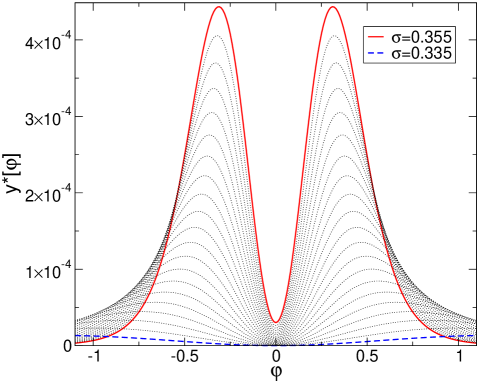
Figure 1: Fixed-point solutions for the function $y^{*}(\varphi)$ for several values of $\sigma$ close to $\sigma_{G}=1/3$. The system at $\sigma_{G}=1/3$ is equivalent to a system at the upper critical dimension: the fixed point is Gaussian (in particular, $y*=0$). Another fixed point emerges for $\sigma>\sigma_{G}$.

For $1/3<\sigma<1/2$, we find two different regimes for the critical behavior, separated by a critical value $\sigma_{c}\approx 0.379$. What distinguishes these regimes is the presence or the absence of a nonanalyticity in the form of a linear cusp in the (dimensionless) renormalized second cumulant of the random field at the fixed point, $\delta^{*}(\varphi_{a},\varphi_{b})$, when $\varphi_{b}\rightarrow\varphi_{a}$: a cusp is present when $\sigma>\sigma_{c}$ but is absent when $\sigma<\sigma_{c}$. The existence of two such regimes separated by a critical value, has been found in the short-range RFIM,tarjus04 ; tissier06 ; tissier11 in the RFO(N)Mtissier06 and in the long-range RFIM in $d=3$ as well.bacz_LR3d In these cases, the cuspless fixed point is associated with a critical behavior satisfying the dimensional-reduction property whereas the presence of a cusp breaks the dimensional reduction and the underlying supersymmetry. In the present $1$-dimensional model, there is no dimensional reduction and no underlying supersymmetry whatsoever. The presence of a cusp in the dimensionless cumulant of the disorder has an effect on the values of the critical exponents, but not as dramatic as in the cases involving dimensional reduction and its breakdown.

This nonanalytical dependence in the dimensionless fields is more conveniently studied by introducing

$$\begin{split}&\varphi=\frac{\varphi_{a}+\varphi_{b}}{2}\\ &\delta\varphi=\frac{\varphi_{b}-\varphi_{a}}{2}\,.\end{split}$$ (28)

The cumulant $\delta^{*}$ is an even function of $\varphi$ and $\delta\varphi$ separately. The presence of a cusp then means that

$$\delta^{*}(\varphi,\delta\varphi)=\delta^{*}_{0}(\varphi)+\delta^{*}_{1}(\varphi)|\delta\varphi|+\frac{1}{2}\delta^{*}_{2}(\varphi)\delta\varphi^{2}+\cdots$$ (29)

with $\delta^{*}_{1}(\varphi)\neq 0$. We show in Fig. 2 $\delta^{*}_{1}(\varphi=0)$ versus $\sigma$. It is equal to zero below $\sigma_{c}\approx 0.379$, indicating that the fixed point is “cuspless”, and it becomes nonzero above $\sigma_{c}$, signaling a “cuspy” fixed point.

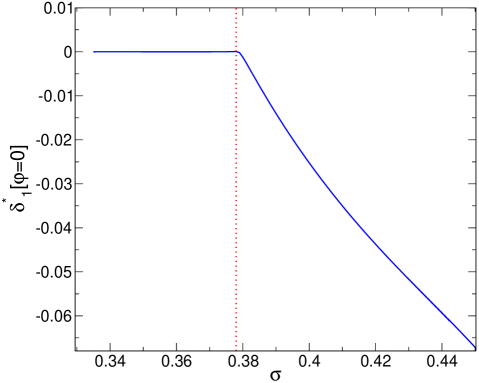
Figure 2: Fixed-point value of the amplitude of the cusp, $\delta_{1}^{*}(\varphi=0)$, versus $\sigma$. Below $\sigma_{c}\approx 0.379$ (denoted by the dotted vertical line), the fixed-point solution is cuspless around $\delta\varphi=0$; a cusp appears and its magnitude further grows above $\sigma_{c}$.

For $\sigma<\sigma_{c}$, the cuspless fixed point and its vicinity are described by a renormalized second cumulant that behaves as

$$\delta_{k}(\varphi,\delta\varphi)=\delta_{k,0}(\varphi)+\frac{1}{2}\delta_{k,2}(\varphi)\delta\varphi^{2}+\cdots$$ (30)

at small $\delta\varphi$. When inserting Eq. (30) into the RG flow equations, Eqs. (LABEL:eq_dimensionless), it is easily realized that one obtains a closed system of 3 coupled equations for $u^{\prime\prime}_{k}(\varphi)$, $y_{k}(\varphi)$ and $\delta_{k,0}(\varphi)$ that can be solved independently of the full dependence of $\delta_{k}(\varphi,\delta\varphi)$. A flow equation for $\delta_{k,2}(\varphi)$ is further obtained with a beta function that depends on $u^{\prime\prime}_{k}(\varphi)$, $y_{k}(\varphi)$, $\delta_{k,0}(\varphi)$ and $\delta_{k,2}(\varphi)$ only. The derivation is straightforward but cumbersome and the resulting equation is not shown here (see Refs. [tarj_avlnch, ; balog_FP, ] for a similar derivation). The function $\delta_{k,2}(\varphi)$ blows up at a finite scale $k_{L}$ for $\sigma>\sigma_{c}$ and the fixed-point function is then given by Eq. (29). On the other hand it reaches a finite fixed-point function for $\sigma<\sigma_{c}$. This allows us to find a precise estimate of $\sigma_{c}=0.379\pm 0.001$ within the present approximation.

Before discussing in more detail the significance and the physics of the two regimes, it is instructive to characterize how the fixed point changes from “cuspless” to “cuspy” by considering the stability of the fixed point with respect to a “cuspy” perturbation, i.e. a perturbation $\propto|\delta\varphi|$ at small $\delta\varphi$. To compute the eigenvalue $\lambda$ associated with such a “cuspy” perturbation, one then has to consider the vicinity of the fixed point with $\delta_{k}(\varphi,\delta\varphi)\simeq\delta^{*}(\varphi\delta\varphi)+k^{\lambda}f_{\lambda}(\varphi,\delta\varphi)$ with $f_{\lambda}(\varphi,\delta\varphi)\simeq|\delta\varphi|f_{\lambda}(\varphi)$ when $\delta\varphi\rightarrow 0$. By linearizing the flow equation for $\delta_{k}$ around $\delta^{*}$ and expanding around $\delta\varphi=0$ one easily derives the eigenvalue equation for $f_{\lambda}(\varphi)$, which depends on $u^{\prime\prime*}(\varphi)$, $y^{*}(\varphi)$, $\delta_{0}^{*}(\varphi)$ and $\delta_{2}^{*}(\varphi)$ only. The details are similar to those given in the supplementary material of Ref. [tarj_avlnch, ] and the resulting equation is not reproduced here.

We show in Figure 3 the evolution of $\lambda$ with $\sigma$. It is positive for $\sigma<\sigma_{c}$, thereby indicating that the cuspy perturbation is irrelevant. For $\sigma=\sigma_{G}=1/3$, i.e. around the Gaussian fixed point, $\lambda$ can be exactly computed and is equal to $1/6$. The eigenvalue then decreases as $\sigma$ increases. The $1$-loop perturbative result in $\sigma=\sigma_{G}+\epsilon$, which is reproduced by the present nonperturbative ansatz, is found to be $\lambda=1/6-\epsilon$ (see Appendix D). When $\sigma=\sigma_{c}^{-}$, we obtain a very small yet strictly positive value, $\lambda_{c-}=0.0011\pm 0.0001$. (This is a robust result as the value is always found strictly positive when varying the parameters of the cutoff function.) Above $\sigma_{c}$, the fixed point is cuspy, and the eigenvalue $\lambda$ can therefore be taken as being zero. In consequence, $\lambda$ is discontinuous in $\sigma_{c}$, which, as explained in Ref. [balog_FP, ], is the signature that the cuspy fixed emerges continuously from the cuspless one through a boundary-layer mechanism.

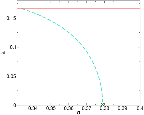
Figure 3: The eigenvalue $\lambda$ associated with a cuspy perturbation versus $\sigma$. The dashed line is the calculation around the cuspless fixed point for $\sigma\leq\sigma_{c}\approx 0.379$: $\lambda$ decreases from $1/6$ when $\sigma=\sigma_{G}=1/3$ to a very small but nonzero value in $\sigma_{c}$; above $\sigma_{c}$ the fixed point is characterized by a cusp and $\lambda$ is strictly zero.

We now turn to the values of the critical exponents. In addition to $\eta$, which is fixed to $2-\sigma$ due to the long-range nature of the interactions, the critical behavior of the system is characterized by the correlation-length exponent $\nu$ and the exponent $2\eta-\bar{\eta}$ that characterizes the scaling behavior of the renormalized cumulant of the random field. From these exponents, one can deduce the other criticalexponents through scaling relations (which are exactly satisfied by the NP-FRG).

The results for $1/\nu$ and $2\eta-\bar{\eta}$ versus $\sigma$ are displayed in Figs. 4 and 5, respectively. Both $1/\nu$ and $2\eta-\bar{\eta}$ have a nonmonotonic behavior with $\sigma$ but this is not related to the change of regime at $\sigma_{c}$. At and around $\sigma_{c}$ the variation of the two exponents is smooth, as expected from the boundary-layer mechanism.balog_FP It is noteworthy that the value of $2\eta-\bar{\eta}$ is small over the whole range of $\sigma$, being at most of the order of $.01$.

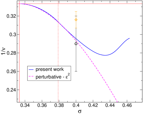
Figure 4: Inverse of the correlation-length exponent $\nu$ versus $\sigma$ as obtained from the present NP-FRG theory (full line). The dashed line is the perturbative result at order $\epsilon^{2}$ around $\sigma_{G}=1/3$.young_77 ; Bray The symbols with the error bars are results from lattice simulations: Ref. [dewenter, ] (circle), Ref. [leuzzi, ] (diamond). The dotted vertical line marks the value $\sigma_{c}\approx 0.379$ separating the “cuspless” and the “cuspy” regimes.

As already mentioned, the present NP-FRG equations exactly reproduce the known $1$-loop perturbative results for $\sigma=\sigma_{G}+\epsilon$: $1/\nu=1/3+{\rm O}(\epsilon^{2})$ and $2\eta-\bar{\eta}={\rm O}(\epsilon^{2})$ (see Appendix D). They are not exact at order $\epsilon^{2}$ but the coefficients of the $\epsilon^{2}$ terms are found to be close to the exact ones:young_77 ; Bray $-10.61$ for $1/\nu$ and $1.498$ for $2\eta-\bar{\eta}$ to be compared to the exact $-10.8984\cdots$ and $1.32498\cdots$. The NP-FRG and the perturbative result at order $\epsilon^{2}$ stay close up to $\sigma\sim 0.4$ for $1/\nu$ but strongly differ even in the vicinity of $\sigma_{G}=1/3$, which seems to indicate in this case large higher-order corrections. None of this however appears to be related to the change of regime at $\sigma_{c}$. Note finally that the result for $1/\nu$ at $\sigma=0.4$, i.e. in the “cuspy” regime, is in very good agreement with the value recently obtained from numerical ground-state determination by Dewenter and Hartmanndewenter (a little less with the result of Ref. [leuzzi, ]).

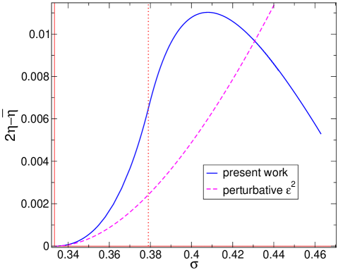
Figure 5: $2\eta-\bar{\eta}$ versus $\sigma$ as obtained from the present NP-FRG theory (full line). The dashed line is the perturbative result to order $\epsilon^{2}$ around $\sigma_{G}=1/3$.Bray The dotted vertical line marks the value $\sigma_{c}\approx 0.379$ separating the “cuspless” and the “cuspy” regimes.

We have been able to follow the critical fixed point up to $\sigma\approx 0.46$, after which the numerical instabilities proliferate. The reason is that $\sigma$ approaches the value of $1/2$, which is the analog of a lower critical dimension below which there is no transition. It is then expected that the low-momentum dependence of the propagators is no longer well described by only taking into account the lowest-order terms of the derivative expansion as done in the ansatz used in this work.

VI Discussion

The existence of two different regimes in the critical behavior of the RFIM can be attributed to the role of “avalanches”, which are collective phenomena present at zero temperature. In equilibrium, such “static” avalanches describe the discontinuous change in the ground state of the system at values of the external source that are sample-dependent (for an illustration see the figures in Refs. [wu-machta05, ; liu-dahmen07, ]). At the critical point, the avalanches take place at all scales and their size distribution follows a power law with a nontrivial exponent $\tau$.

It was shown in Ref. [tarj_avlnch, ] for the RFIM (and in Refs. [BBM96, ; aval_FRG, ] for interfaces in a random environment) that the presence of avalanches necessarily induces a cusp in the functional dependence of the renormalized cumulants of the disorder and in properly chosen correlation functions. Actually, such a cuspy dependence is already present in the $d=0$ RFIM.tarj_avlnch As the critical behavior is affected by a cusp in the dimensionless quantities,tarjus04 ; tissier06 ; tissier11 the question is then whether the amplitude of the cusp is, or not, an irrelevant contribution at the fixed point.

In physical terms, the two regimes therefore correspond to two different situations where the scale of the largest typical avalanches at criticality, which in a system of linear size $L$ goes as $L^{d_{f}}$ with $d_{f}\leq d$, is equal to the scale of the total magnetization, i.e. as $L^{d-(d-4+\bar{\eta})/2}$, or is subdominant. This is precisely characterized by the eigenvalue $\lambda$ calculated in the previous section. In the regime where the fixed point is cuspless, $d_{f}=d-(d-4+\bar{\eta})/2-\lambda$ with $\lambda>0$ whereas $d_{f}=d-(d-4+\bar{\eta})/2$ in the regime where the fixed point is cuspy.

The main interest of the $1$-dimensional long-range RFIM is that it can be studied by computer simulations for large system sizes. Efficient algorithms exist to determine the ground state in a polynomial time and one can further reduce the computational cost by considering a diluted (Levy) lattice which is expected to be in the same universality class.leuzzi ; dewenter Sizes up to $L=256000$ in Ref. [leuzzi, ] and $L=524288$ in Ref. [dewenter, ] have thus been investigated.

As discussed before, the critical exponents characterizing the leading scaling behavior do not show any significant change of dependence with $\sigma$ around the critical value $\sigma_{c}$ (they are predicted to be continuous in $\sigma_{c}$). To distinguish the two regimes it seems therefore preferable to investigate the avalanche distribution at $T=0$ and try to extract the fractal dimension $d_{f}$ of the largest avalanches. This can be obtained through a finite-size scaling of the distribution of the avalanches or of its first moments. For instance, the ratio of the second to the first moment of the avalanche size, $<S^{2}>/<S>$, should scale as $L^{d_{f}}$ for $L$ large enough. Having extracted $d_{f}$ and $2\eta-\bar{\eta}$, one can obtain the eigenvalue $\lambda$ from the relation

$$\lambda=\frac{d+4-\bar{\eta}}{2}-d_{f}=\frac{1}{2}+\sigma+\frac{2\eta-\bar{\eta}}{2}-d_{f}$$ (31)

where $2\eta-\bar{\eta}$ is anyhow expected to be very small. If $\lambda>0$, one is in the cuspless regime and if $\lambda=0$ in the cuspy one. By studying values of $\sigma$ near $\sigma_{G}=1/3$ where $\lambda$ should be $\approx 1/6$ and values of $\sigma\gtrsim 0.4$ it should be possible to distinguish the two regimes in computer simulations.

In addition, one could also consider the corrections to scaling. In the vicinity of the critical value $\sigma_{c}\approx 0.379$, these corrections should be dominated by the lowest (positive) eigenvalue in the $Z_{2}$-symmetric subspace of perturbations around the fixed point. For $0.372\lesssim\sigma\leq\sigma_{c}$, this eigenvalue is equal to $\lambda$ and is therefore expected to be very small (with $\lambda_{c}^{-}\approx 0.0011$). Right above $\sigma_{c}$, the smallest irrelevant eigenvalue is also associated with a cuspy perturbation and it emerges from a value $\lambda_{c}^{+}\lesssim\lambda_{c}^{-}$ at $\sigma_{c}^{+}$.balog_FP The exponent describing the main correction to scaling should therefore display a minimum as a function of $\sigma$ with a value near zero for $\sigma=\sigma_{c}\approx 0.379$.

Finally, we conclude by discussing the RFIM on the Dyson hierarchical lattice. This lattice mimics the behavior of the $1$-dimensional chain with long-range interactions specified by the same parameter $\sigma$. Its critical behavior was studied by Rodgers and Brayrodgers-bray and its avalanche distribution was characterized in detail more recently by Monthus and Garel.monthus11

It was shown in Ref. [rodgers-bray, ] that in this case the temperature exponent is always given by $\theta=\sigma$, which implies, together with the result $\eta=2-\sigma$, that $2\eta-\bar{\eta}=0$. In addition, it was found in Ref. [monthus11, ] that the fractal dimension of the largest avalanches at criticality is $d_{f}=2\sigma$. These two results, $2\eta-\bar{\eta}=0$ and $d_{f}=2\sigma$, when inserted into Eq. (31) predict that $\lambda=1/2-\sigma$. As a consequence, $\lambda$ decreases from $1/6$ to $0$ as $\sigma$ decreases from $1/3$ to $1/2$ and is always strictly positive, except at the analog of the lower critical dimension. In consequence, the RFIM on the Dyson hierarchical level appears to display a unique regime over the whole range $1/3\leq\sigma<1/2$: avalanches are present at all scales but their scaling dimension is never large enough to induce a cuspy fixed point. This is a notable difference with the long-range RFIM on the standard $1$-d chain.

To summarize: The NP-FRG predicts that the critical behavior of the RFIM generically shows two distinct regimes separated by a nontrivial critical value of the dimension, the number of components or the power-law exponent of the long-range interactions, when present. These regimes are associated with properties of the large-scale avalanches at zero temperature. We suggest that investigating through numerical simulations the avalanche characteristics in the $1$-dimensional long-range RFIM should provide a direct check of the prediction.

Appendix A The flow equations for $U^{\prime\prime}_{k}(\phi)$ and $\Delta_{k}(\phi_{a},\phi_{b})$

Starting from Eq. (LABEL:diagram_1cgamma2) and setting the external momentum to $0$ one easily obtains the flow equation for $U^{\prime\prime}_{k}$, $\partial_{t}U^{\prime\prime}_{k}(\phi)=\beta_{U^{\prime\prime}}(\phi)$, with

$$\begin{split}&\beta_{U^{\prime\prime}}=-\frac{1}{2}\int_{0}^{\infty}\frac{dq}{\pi}\partial_{t}\widehat{R}(q)\widehat{G}_{k}q;\phi)^{2}\Big{\{}\Delta^{(2,0)}_{k}(\phi,\phi)+\\ &\Delta^{(0,2)}_{k}(\phi,\phi)+2\Delta^{(1,1)}_{k}(\phi,\phi)+2\widehat{G}_{k}(q;\phi)\Big{[}-2\times\\ &\big{[}\Delta^{(1,0)}_{k}(\phi,\phi)+\Delta^{(0,1)}_{k}(\phi,\phi)\big{]}\big{[}U^{\prime\prime\prime}_{k}(\phi)+q^{1+2\sigma}Y^{\prime}_{k}(\phi)\big{]}\\ &-\Delta_{k}(\phi,\phi)\Big{(}U^{(4)}_{k}(\phi)+q^{1+2\sigma}Y^{\prime\prime}_{k}(\phi)-3\widehat{G}_{k}(q;\phi)\times\\ &\big{[}U^{\prime\prime\prime}_{k}(\phi)+q^{1+2\sigma}Y^{\prime}_{k}(\phi_{a})\big{]}^{2}\Big{)}\Big{]}\Big{\}}\end{split}$$ (32)

To obtain the expression for the flow equation of $\Delta_{k}$, $\partial_{t}\Delta_{k}(\phi_{a},\phi_{b})=\beta_{\Delta}(\phi_{a},\phi_{b})$, we derive Eq. (LABEL:eq_ERGE_Gamma2) with respect to $\phi_{a}$ and $\phi_{b}$, insert the ansatz for the effective average action and express the output in terms of the Fourier transformed quantities. The flow of $\Delta_{k}$ is then given by setting the external momentum $p$ to zero, which leads to the following graphical expression:

$$\begin{split}&\partial_{t}\Delta_{k}(\phi_{a},\phi_{b})=-\frac{1}{2}\tilde{\partial_{t}}\int_{q}\\ &\Bigg{(}\raisebox{-20.0pt}{\includegraphics[width=240.0pt,height=40.0pt]{2copy_2point1.eps}}\\ &\raisebox{-15.0pt}{\includegraphics[width=240.0pt,height=40.0pt]{2copy_2point2.eps}}\\ &\raisebox{-15.0pt}{\includegraphics[width=220.0pt,height=40.0pt]{2copy_2point3.eps}}\Bigg{)},\end{split}$$ (33)

Explicitly written, the expression for $\beta_{\Delta}$ reads

$$\begin{split}&\beta_{\Delta}=-\int_{0}^{\infty}\frac{dq}{\pi}\partial_{t}\widehat{R}_{k}(q)\Bigg{\{}-\widehat{G}_{k}(q;\phi_{a})^{3}\Big{[}\Delta_{k}(\phi_{a},\phi_{a})\times\\ &\Delta_{k}^{(2,0)}(\phi_{a},\phi_{b})+\Delta_{k}^{(1,0)}(\phi_{a},\phi_{b})\Big{(}\Delta_{k}^{(0,1)}(\phi_{a},\phi_{a})+\Delta_{k}^{(1,0)}(\phi_{a},\phi_{a})\\ &-3\big{[}U^{(3)}_{k}(\phi_{a})+q^{1+2\sigma}Y^{\prime}_{k}(\phi_{a})\big{]}\Delta_{k}(\phi_{a},\phi_{a})\widehat{G}_{k}(q;\phi_{a})\Big{)}\Big{]}\\ &-\Big{[}\Delta_{k}(\phi_{a},\phi_{b})\Delta_{k}^{(1,1)}(\phi_{a},\phi_{b})+\Delta_{k}^{(0,1)}(\phi_{a},\phi_{b})\Big{(}\Delta_{k}^{(1,0)}(\phi_{a},\phi_{b})\\ &-2\big{[}U^{(3)}_{k}(\phi_{a})+q^{1+2\sigma}Y^{\prime}_{k}(\phi_{a})\big{]}\Delta_{k}(\phi_{a},\phi_{b})\widehat{G}_{k}(q;\phi_{a})\Big{)}\Big{]}\times\\ &\widehat{G}_{k}(q;\phi_{a})^{2}\widehat{G}_{k}(q;\phi_{b})+\big{[}U^{(3)}_{k}(\phi_{a})+q^{1+2\sigma}Y^{\prime}_{k}(\phi_{a})\big{]}\Delta_{k}(\phi_{a},\phi_{b})\\ &\times\Big{(}\Delta_{k}^{(0,1)}(\phi_{a},\phi_{b})-\big{[}U^{(3)}_{k}(\phi_{b})+q^{1+2\sigma}Y^{\prime}_{k}(\phi_{b})\big{]}\times\\ &\Delta_{k}(\phi_{a},\phi_{b})\widehat{G}_{k}(q;\phi_{a})\Big{)}\widehat{G}_{k}(q;\phi_{a})^{2}\widehat{G}_{k}(q;\phi_{b})^{2}+perm(a,b)\Bigg{\}}\,.\end{split}$$ (34)

Appendix B Toy model integral

We consider the following one-dimensional integral

$$\mathcal{I}(p)=\int^{\infty}_{-\infty}dq\frac{1}{[|q+p|^{\sigma}+f((q+p)^{2})][|q|^{\sigma}+f(q^{2})]}$$ (35)

with $1/3<\sigma<1/2$, in the vicinity of $p=0$. (As $\mathcal{I}(p)=\mathcal{I}(-p)$, we restrict ourselves to $p\geq 0$.) The function $f(q^{2})$ is chosen such that $f(0)\neq 0$ and that its large $q^{2}$ behavior garantees the convergence of the integral. As a result $\mathcal{I}(p=0)$ is finite and we look for the leading $p$-dependence when $p\rightarrow 0$. A naive expansion in $p$ predicts a $p^{2}$ dependence, but this turns out to be wrong. To obtain the correct behavior, we first rewrite $\mathcal{I}(p)-\mathcal{I}(0)$ as

$$\begin{split}&\mathcal{I}(p)-\mathcal{I}(0)=\int^{\infty}_{-\infty}dq\\ &\Bigg{[}\frac{1}{(|q+\frac{p}{2}|^{\sigma}+f((q+\frac{p}{2})^{2}))(|q-\frac{p}{2}|^{\sigma}+f((q-\frac{p}{2})^{2}))}-\\ &\frac{1}{2}\Big{(}\frac{1}{[|q+\frac{p}{2}|^{\sigma}+f((q+\frac{p}{2})^{2})]^{2}}+\frac{1}{[|q-\frac{p}{2}|^{\sigma}+f((q-\frac{p}{2})^{2})]^{2}}\Big{)}\Bigg{]}\end{split}$$ (36)

where, for convenience, we have expressed $\mathcal{I}(p=0)$ in a symmetrized form by changing the integration variable to $q\pm\frac{p}{2}$.

We now introduce the variable $x=\sqrt{q^{2}+(p^{2}/4)}$, so that

$$\begin{split}&|q\pm\frac{p}{2}|^{\sigma}+f(|q\pm\frac{p}{2}|^{2})=f(x^{2})+|x|^{\sigma}\pm\frac{qp}{|x|^{2-\sigma}}(\frac{\sigma}{2}+\\ &|x|^{2-\sigma}f^{\prime}(x^{2}))+\frac{q^{2}p^{2}}{2|x|^{4-\sigma}}(\frac{\sigma(\sigma-2)}{4}+|x|^{4-\sigma}f^{\prime\prime}(x^{2}))+\cdots\end{split}$$ (37)

where the ellipses denotes terms with higher-order powers in $p$ (at fixed $x$).

After inserting Eq. (LABEL:denom_exp) in Eq. (LABEL:toy4) and changing variable from $q$ to $z=q/p$, we obtain

$$\begin{split}&\mathcal{I}(p)-\mathcal{I}(0)=\\ &-\frac{p^{1+2\sigma}}{2}\int^{\infty}_{-\infty}dz\frac{z^{2}}{(z^{2}+\frac{1}{4})^{2-\sigma}}\Big{[}\frac{\sigma^{2}+{\rm O}(p^{2-\sigma})}{f(0)^{4}+{\rm O}(p^{\sigma})}\,,\Big{]}\end{split}$$ (38)

so that

$$\lim_{p\rightarrow 0}\frac{\mathcal{I}(p)-\mathcal{I}(0)}{p^{1+2\sigma}}=-\frac{\sigma^{2}}{2f(0)^{4}}\int^{\infty}_{-\infty}dz\frac{z^{2}}{(z^{2}+\frac{1}{4})^{2-\sigma}}\,,$$ (39)

where the integral over $z$ converges in the range of $\sigma$ considered.

Appendix C Derivation of $\beta_{Y,an}$

Figure 6: The diagrams contributing to the anomalous kinetic term in $|p|^{1+2\sigma}$. A cross denotes an insertion of $\partial_{t}\widehat{R}_{k}(q)$.

Consider the diagrams shown in Fig. 6. They enter in the right-hand side of the flow equation of $\Gamma^{(2)}_{k1}(p;\phi)$ as

$$\begin{split}&\mathcal{I}_{an}(p)=-\frac{1}{2\pi}\int_{-\infty}^{+\infty}dq\,\partial_{t}\widehat{R}_{k}(q)\widehat{G}_{k}(q;\phi)^{2}\widehat{G}_{k}(p+q;\phi)\\ &\times U^{\prime\prime\prime}_{k}(\phi)\Big{(}-2\big{[}\Delta^{(1,0)}_{k}(\phi,\phi)+\Delta^{(0,1)}_{k}(\phi,\phi)\big{]}+\\ &U^{\prime\prime\prime}_{k}(\phi)\Delta_{k}(\phi,\phi)\big{[}2\widehat{G}_{k}(q;\phi)+\widehat{G}_{k}(q+p;\phi)\big{]}\Big{)}\end{split}$$ (40)

with $\widehat{G}_{k}(q;\phi)$ given by Eq. (23).

The expressions which need to be expanded in small $p$ (we consider $p\geq 0$) are therefore the three integrals $\mathcal{I}_{an,1}(p)=\int dq\partial_{t}\widehat{R}_{k}(q)\widehat{G}_{k}(q;\phi)^{2}\widehat{G}_{k}(q+p;\phi)$, $\mathcal{I}_{an,2}(p)=\int dq\partial_{t}\widehat{R}_{k}(q)\widehat{G}_{k}(q;\phi)^{3}\widehat{G}_{k}(q+p;\phi)$ and $\mathcal{I}_{an,3}(p)=\int dq\partial_{t}\widehat{R}_{k}(q)\widehat{G}_{k}(q;\phi)^{2}\widehat{G}_{k}(q+p;\phi)^{2}$. We follow exactly the same procedure as in the Appendix B: we symmetrize the integrands when needed, introduce the variable $x=\sqrt{q^{2}+\frac{p^{2}}{4}}$, expand in small $p$ and finally change the integration variable from $q$ to $z=q/p$. The outcome at leading order in $p$ is then

$$\begin{split}&\mathcal{I}_{an,1}(p)-\mathcal{I}_{an,1}(0)=\\ &-p^{1+2\sigma}\partial_{t}\widehat{R}_{k}(0)\widehat{G}_{k}(0;\phi)^{5}\int_{-\infty}^{+\infty}dz\frac{\sigma^{2}z^{2}}{(z^{2}+\frac{1}{4})^{2-\sigma}}\,,\\ &\mathcal{I}_{an,2}(p)-\mathcal{I}_{an,2}(0)=\\ &-p^{1+2\sigma}\partial_{t}\widehat{R}_{k}(0)\widehat{G}_{k}(0;\phi)^{6}\int_{-\infty}^{+\infty}dz\frac{3\sigma^{2}z^{2}}{2(z^{2}+\frac{1}{4})^{2-\sigma}}\,,\\ &\mathcal{I}_{an,3}(p)-\mathcal{I}_{an,3}(0)=\\ &-p^{1+2\sigma}\partial_{t}\widehat{R}_{k}(0)\widehat{G}_{k}(0;\phi)^{6}\int_{-\infty}^{+\infty}dz\frac{2\sigma^{2}z^{2}}{(z^{2}+\frac{1}{4})^{2-\sigma}}\,.\end{split}$$ (41)

After inserting the above expressions in (LABEL:betY2start) and performing the integral over $z$, one immediately obtains Eq. (LABEL:betY2).

Appendix D Recovering the perturbative result at order $\epsilon=\sigma-1/3$ from the NP-FRG

We study the NP-FRG flow equations expressed in dimensionless quantities in the vicinity of the boundary value to classical (long-range) behavior, $\sigma_{l}=\frac{1}{3}$. The fixed point should be close to the Gaussian fixed point characterized by $u^{\prime\prime}_{k}=y_{k}=0$ and $\delta_{k}(\varphi,\delta\varphi)=1$ (recall that the long-range kinetic part is not renormalized so that $\eta=2-\sigma$). For $\sigma=1/3+\epsilon$, we expand the functions in powers of the fields,

$$\begin{split}&u^{\prime\prime}_{k}(\varphi)=u_{k,2}+\frac{1}{2}u_{k,4}\varphi^{2}+{\rm O}(\varphi^{4})\,,\\ &y_{k}(\varphi)=\frac{1}{2}y_{k,2}\varphi^{2}+{\rm O}(\varphi^{4})\,,\\ &\delta_{k}(\varphi,\delta\varphi)=\\ &1+\frac{1}{2}(\delta_{k,20}\varphi^{2}+\delta_{k,02}\delta\varphi^{2})+{\rm O}(\varphi^{4},\delta\varphi^{4},\varphi^{2}\delta\varphi^{2})\,,\end{split}$$ (42)

where one expects $u_{k,2}$, $u_{k,4}$, $y_{k,2}$, $\delta_{k,20}$, $\delta_{k,02}$ to be at least of O($\epsilon$) around the fixed point.

After inserting the above expressions in the beta function $\widetilde{\beta}_{u^{\prime\prime}}(\varphi)$ obtained from Eq. (LABEL:eq_beta_u''), one finds the following flow equation for the coupling constant $u_{k,4}$:

$$\partial_{t}u_{k,4}=-3\epsilon u_{k,4}+36u^{2}_{k,4}I_{4}(u_{k,2})+O(\epsilon^{2})$$ (43)

where

$$I_{n}(u_{2})=\frac{1}{2}\int_{0}^{\infty}\frac{dq}{\pi}\widetilde{\partial}_{t}s(q^{2})\,\widehat{p}_{0}(q)^{n}$$ (44)

with $\widehat{p}_{0}(q)=[q^{\sigma}+s(q^{2})+u_{2}]^{-1}$ and $\widetilde{\partial}_{t}s(q^{2})=\sigma s(q^{2})-2q^{2}s^{\prime}(q^{2})$. Eq. (43) admits a nontrivial fixed-point solution $u^{*}_{4}=\epsilon/[12I_{4}(0)]+O(\epsilon^{2})$.

Similarly, the flow of $u_{k,2}$ reads

$$\partial_{t}u_{k,2}=-\sigma u_{k,2}-4u_{k,4}I_{3}(u_{k,2})+{\rm O}(\epsilon^{2})\,,$$ (45)

which leads to $u^{*}_{2}=-\epsilon I_{3}(0)/[3\sigma I_{4}(0)]+O(\epsilon^{2})$.

On the other hand, from the beta function for $\delta_{k}$ and the condition $\partial_{t}\delta_{k}(0,0)=0$, one derives that

$$2\eta-\overline{\eta}=O(\epsilon^{2})\,.$$ (46)

To derive the $\epsilon$ dependence of the exponent $1/\nu$, one starts from the flow equation for $u_{k,2}$ and perturbs the fixed point by a small constant $k^{-1/\nu}\delta u_{2}$. By using that $I_{3}(u^{*}_{2}+\delta u_{2})\approx I_{3}(u^{*}_{2})-3I_{4}(u^{*}_{2})\delta u_{2}$ one finds the following linearized equation:

$$\frac{-1}{\nu}\delta u_{2}=(-\sigma+\epsilon)\delta u_{2}+O(\epsilon^{2})\,,$$ (47)

which implies, as $\sigma=1/3+\epsilon$,

$$\frac{1}{\nu}=\frac{1}{3}+O(\epsilon^{2})\,.$$ (48)

The above expression for $1/\nu$ is identical to the perturbative result.young_77

Finally, we can also derive the expression for the eigenvalue $\lambda$. In the vicinity of the Gaussian fixed point we look for an eigenfunction $f\lambda(\varphi)$ of the form $f_{\lambda}(\varphi)=f_{\lambda,0}+(1/2)f_{\lambda,2}\varphi^{2}+\cdots$. We find that $f_{\lambda,2}={\rm O}(\epsilon^{2})$ and the eigenvalue equation then reads

$$\begin{split}\lambda f_{\lambda,0}=(\frac{1}{6}-\epsilon)f_{\lambda,0}+{\rm O}(\epsilon^{2})\,,\end{split}$$ (49)

which leads to

$$\lambda=\frac{1}{6}-\epsilon+{\rm O}(\epsilon^{2})\,.$$ (50)

This is the result quoted in the main text.

References

- (1) Y. Imry and S. K. Ma, Phys. Rev. Lett. 35, 1399 (1975).
- (2) For a review, see T. Nattermann, Spin glasses and random fields (World scientific, Singapore, 1998), p. 277.
- (3) G.Grinstein, Phys. Rev. Lett. 37, 944 (1976).
- (4) A.P.Young, J. Phys. C 10, L257 (1977).
- (5) G.Parisi and N. Sourlas, Phys. Rev. Lett. 43, 744 (1979).
- (6) J.Z. Imbrie: Phys. Rev. Lett. 53, 1747.
- (7) J.Brichmont and A. Kupiainen, Phys. Rev. Lett. 59, 1829 (1987).
- (8) G. Tarjus and M. Tissier, Phys. Rev. Lett 93, 267008 (2004); Phys. Rev. B 78, 024203 (2008).
- (9) M. Tissier and G. Tarjus, Phys. Rev. Lett. 96, 087202 (2006); 78, 024204 (2008).
- (10) M. Tissier and G. Tarjus, Phys. Rev. Lett. 107, 041601 (2011); Phys. Rev. B 85, 104202 (2012); Phys. Rev. B 85, 104203 (2012).
- (11) D. S. Fisher, Phys. Rev. Lett. 56, 1964 (1986). O. Narayan and D. S. Fisher, Phys. Rev. B 46, 11520 (1992).
- (12) P. Le Doussal, K. J. Wiese, and P. Chauve, Phys. Rev. B 66, 174201 (2002); Phys. Rev. E 69, 026112 (2004).
- (13) P. Le Doussal and K. J. Wiese, Phys. Rev. E 79, 051106 (2009); Phys. Rev. E 85, 061102 (2011).
- (14) M. Baczyk, M. Tissier, G. Tarjus, and Y. Sakamoto, Phys. Rev. B 88, 014204 (2013).
- (15) G. Tarjus, M. Baczyk, and M. Tissier, Phys. Rev. Lett. 110, 135703 (2013).
- (16) T.Dewenter and A.K.Hartmann, arXiv:1307.3987.
- (17) L. Leuzzi and G. Parisi, Phys. Rev. B 88, 224204 (2013).
- (18) A. J. Bray: J. Phys. C 19, 6225 (1986).
- (19) M. Cassandro, E. Orlandi, and P. Picco, Commun. Math. Phys. 288, 731 (2009).
- (20) G. J. Rodgers and A. J. Bray: J. Phys. A: Math. Gen. 21, 2177 (1988).
- (21) C. Monthus and T. Garel, J. Stat. Mech., P07010 (2011).
- (22) M.Mezard, G.Parisi and M.A.Virasoro: Spin Glass Theory and Beyond, World Scientific (1987).
- (23) J.Berges, N.Tetradis and C.Wetterich, Phys. Rep. 363, 223 (2002).
- (24) C. Wetterich, Physics Letters B 301, 90 (1993).
- (25) D. F. Litim, Phys. Lett. B 486, 92 (2000); Nucl. Phys. B 631, 128 (2002).
- (26) L. Canet, B. Delamotte, D. Mouhanna, and J. Vidal, Phys. Rev. D 67, 065004 (2003). 36
- (27) J. M. Pawlowski, Ann. Phys. 322, 2831 (2007).
- (28) See for instance Numerical recipes, Cambridge University press (1992), vol 1, sec. 9.4.
- (29) M. Baczyk, G. Tarjus, M. Tissier and I. Balog, J. Stat Mech., P06010 (2014).
- (30) Y. Wu and J. Machta, Phys. Rev. Lett. 95, 137208 (2005); Phys. Rev. B 74, 064418 (2006).
- (31) Y. Liu and K. A. Dahmen, Phys. Rev. E 76, 031106 (2007).
- (32) L. Balents L, J.-P. Bouchaud and M. Mezard, J. physique I 6, 1007 (1996).
- (33) A. A. Middleton, P. Le Doussal and K. J. Wiese, Phys. Rev. Lett. 98, 155701 (2007); P. Le Doussal, A. A. Middleton, and K. J. Wiese, Phys. Rev. E 79, 050101 (2009).