Sparse Partially Linear Additive Models

Abstract

The generalized partially linear additive model (GPLAM) is a flexible and interpretable approach to building predictive models. It combines features in an additive manner, allowing each to have either a linear or nonlinear effect on the response. However, the choice of which features to treat as linear or nonlinear is typically assumed known. Thus, to make a GPLAM a viable approach in situations in which little is known a priori about the features, one must overcome two primary model selection challenges: deciding which features to include in the model and determining which of these features to treat nonlinearly. We introduce the sparse partially linear additive model (SPLAM), which combines model fitting and both of these model selection challenges into a single convex optimization problem. SPLAM provides a bridge between the lasso and sparse additive models. Through a statistical oracle inequality and thorough simulation, we demonstrate that SPLAM can outperform other methods across a broad spectrum of statistical regimes, including the high-dimensional ($p\gg N$) setting. We develop efficient algorithms that are applied to real data sets with half a million samples and over 45,000 features with excellent predictive performance.

1 Introduction

Generalized partially linear additive models (GPLAMs, Härdle and Liang 2007) provide an attractive middle ground between the simplicity of generalized linear models (GLMs, Nelder and Wedderburn 1972) and the flexibility of generalized additive models (GAMs, Hastie and Tibshirani 1990). Given a data set $\{(x_{i},y_{i})\}_{i=1}^{N}$, a GPLAM relates the conditional mean of the response, $y_{i}$, to the $p$-dimensional predictor vector, $x_{i}$, using a known link function, $g$:

$$g(E[y_{i}|x_{i}])=\sum_{j\in\mathcal{N}}f_{j}(x_{ij})+\sum_{j\in\mathcal{L}}x_{ij}\theta_{j}.$$ (1)

The features in $\mathcal{N}$ contribute to the model in a nonlinear fashion while the features in $\mathcal{L}$ contribute in a linear fashion. A GLM treats all features as being in $\mathcal{L}$ and may therefore be biased when nonlinear effects are present; on the other extreme, a GAM treats all features as being in $\mathcal{N}$, which incurs unnecessary variance for the features that should be treated as linear. GPLAMs are a popular tool for data analysis in multiple domains including economics (Engle et al., 1986; Green and Silverman, 1993) and biology (Lian et al., 2012; Dinse and Lagakos, 1983).

A major obstacle to using GPLAMs on large-scale data sets is that one rarely knows a priori which features should be assigned to $\mathcal{N}$ and $\mathcal{L}$. A further challenge is in deciding which features should be excluded from the model entirely. The goal of this paper is to make GPLAMs a viable tool for building large-scale predictive models. To do so, we must overcome two model-selection challenges: automatically deciding which features are at all relevant in the model and deciding which of those features should be fit linearly versus nonlinearly.

In the context of GAMs (where $\mathcal{L}$ is taken to be empty), the sparse additive model (SpAM) is a useful framework for performing feature selection on $\mathcal{N}$ (Ravikumar et al., 2009). From the perspective of a GPLAM, SpAM takes an “all-in” or “all-out” approach to feature selection. In this work, we introduce the sparse partially linear additive model (SPLAM) that provides the finer-grained selection demanded by a GPLAM. SPLAMs build on the SpAM framework, providing a natural bridge between the $\ell_{1}$-penalized GLM and SpAM, thereby reaping many of the benefits enjoyed by both of these methods.

Failing to account for exactly linear features is disadvantageous statistically, computationally, and in terms of interpretability. As a motivating example, consider a situation in which $p=1,000$, $|\mathcal{N}|=5$, and $|\mathcal{L}|=295$. Assuming the correct set of features is selected, SpAM would include 300 features. From an interpretability standpoint, one would have to manually inspect the 300 nonparametric fits to reveal that only 5 features are effectively nonlinear. The other 295 of them would appear nearly, but not exactly, linear such as in Figure 1 (d). Statistically, a price is paid in variance for the many nearly-linear features; and, computationally, such a model is wasteful both in terms of memory and speed for making future predictions.

In the last several years, a number of methods have been proposed to address various aspects of this problem. In Chen et al. (2011), a bootstrap-based test is developed to determine the linearity of a component. In Huang et al. (2012), the authors use a group MCP penalty to decide which features should be linear versus nonlinear, but features may not be completely excluded from the model. In Du et al. (2012), an algorithm is developed that iterates between two optimization problems: one that decides which nonlinear features should be made linear and the other that decides which linear features should be set to zero. An alternative approach to SpAM is the component selection and smoothing operator (COSSO) method, which uses unsquared reproducing kernel Hilbert space (RKHS) norm penalties (Lin and Zhang, 2006). The linear and nonlinear discoverer extends COSSO to the GPLAM setting (Zhang et al., 2011). Relatedly, Lian et al. (2012) combine smoothness and sparsity SCAD-based penalties for a similar purpose. None of the above methods is geared toward high-dimensional data in terms of statistical theory or computation. Several other methods are geared toward the high-dimesional setting but do not perform both model selection tasks. For example, in Bunea (2004); Xie and Huang (2009); Müller and van de Geer (2013), methods are developed to perform feature selection for the set $\mathcal{L}$ while assuming that the set $\mathcal{N}$ is known; Lian and Liang (2013) and Wang et al. (2014) perform feature selection on both $\mathcal{L}$ and $\mathcal{N}$ individually but assume an initial partition of the features into those potentially in $\mathcal{L}$ and those potentially in $\mathcal{N}$.

By contrast, SPLAM is designed for large-scale datasets (for example, we apply it to a dataset with $p=47,236$). SPLAM is formulated through a single convex optimization problem that admits an efficient algorithm and strong theoretical properties even in the $p\gg N$ setting.

In Section 2, we define the SPLAM estimator as the solution to a convex optimization problem, and, in Section 3, we discuss how this problem may be efficiently solved in large-scale contexts. Section 4 presents consistency results under weak assumptions and lends theoretical support to the conceptual difference in predictive performance between SPLAM and SpAM, its close relative. Section 5 provides an empirical study of SPLAM, including both a thorough simulation study and comparison of SPLAM to other methods on an array of large data examples.

2 The SPLAM Optimization

We approach the challenging model selection and fitting problem posed by a GPLAM through convex relaxation. For each feature $x_{j}$, we perform an $M$-dimensional basis expansion $b(x_{j})=[b_{1}(x_{j}),...,b_{M}(x_{j})]$ in which $b_{1}(x_{j})=x_{j}$ and $M$ is typically small. Our main requirement of the basis is that $b_{1}(x_{j})$ models the linear part and that $[b_{2}(x_{j}),...,b_{M}(x_{j})]=:b_{-1}(x_{j})$ models the nonlinear part. SPLAM estimates each $f_{j}(\cdot)$ by a function in the space spanned by $b(\cdot)$, i.e., $f_{j}(x_{j})=b(x_{j})\beta_{j}$, where $\beta_{j}\in\mathbb{R}^{M}$ (for ease of exposition we ignore the intercept). We use $\beta_{j1}$ and $\beta_{j,-1}$ to denote the coefficients of the linear and nonlinear basis functions, respectively. Letting $\beta=[\beta_{1}^{T},...,\beta_{p}^{T}]^{T}\in\mathbb{R}^{pM}$ and $X=[b(x_{1}):\cdots:b(x_{p})]\in\mathbb{R}^{N\times pM}$ be the design matrix, we have

$$X\beta=\sum_{j=1}^{p}\left[\beta_{j1}x_{j}+\beta_{j,-1}b_{-1}(x_{j})\right].$$

Given a convex smooth loss function $L(y,X,\beta)$, SPLAM is formulated as the solution to the following convex program with hierarchical sparsity regularization:

Optimization Problem 1.

SPLAM

$$\min_{\beta}L(y,X,\beta)+\lambda\Omega^{{SPLAM}}(\beta)$$ (2)

where $\Omega^{{SPLAM}}(\beta)=\sum_{j=1}^{p}\left[\alpha\|\beta_{j}\|_{2}+(1-\alpha)\|\beta_{j,-1}\|_{2}\right],$ $\lambda\geq 0$, and $\alpha\in[0,1]$.

In this paper, we focus on linear regression, in which $L(y,X,\beta)=\frac{1}{2N}\|y-X\beta\|_{2}^{2}$ and logistic regression, in which $L(y,X,\beta)=\frac{1}{N}\sum_{i}\log(1+\exp[-y_{i}\sum_{k=1}^{pM}X_{ik}\beta_{k}])$, where $y_{i}\in\{-1,1\}$. The penalty function $\Omega^{SPLAM}$ is convex and is an instance of the hierarchical group lasso (Zhao et al., 2009; Jenatton et al., 2010). Its two terms address the two forms of model selection present in the GPLAM problem: the first term affects the overall number of predictors appearing in the fitted model; the second term controls the number of those features that are treated nonlinearly.

Just as GPLAMs generalize both GLMs and GAMs, it is useful to note that SPLAM includes the most common penalized estimators used for these two kinds of models.

• When $\alpha=1$ and an orthogonal basis is used, Problem 1 becomes SpAM in group lasso form.

• When $\lambda=\tilde{\lambda}/\alpha$ and $\alpha$ is sufficiently small, SPLAM reduces to the lasso (Tibshirani, 1996) applied to the linear features only.

In practice, we solve the SPLAM problem over a grid of $(\lambda,\alpha)$ pairs. Our strategy is to fix $\alpha$ and solve the problem pathwise starting from the smallest value of $\lambda$ for which $\hat{\beta}_{j}=0$ for all $j=1,...,p$ and decreasing $\lambda$ exponentially. In Section 4.1, we prove that SPLAM is consistent under general conditions for $\alpha=(1+\sqrt{6})/(1+2\sqrt{6})$ and suitably chosen $\lambda$.

After posting the initial draft of this paper online, we learned of a similar method being developed independently and concurrently to ours (Chouldechova and Hastie, 2015); their approach to the GPLAM problem also makes use of an overlapping group lasso penalty, but uses a different form of penalty known as the latent overlapping group lasso penalty (Obozinski et al., 2011). Also, Petersen et al. (2014) in a recent preprint propose a method that combines feature selection and non-linear, piecewise-constant modeling using a fused-lasso penalty.

3 Computation

The hierarchical group lasso can be solved efficiently by proximal gradient descent (Beck and Teboulle, 2009) as described in Jenatton et al. (2010). The idea of this algorithm is to modify the standard gradient steps that one would take if simply minimizing $L$ and then apply the proximal operator of the nondifferentiable penalty, $\lambda\Omega^{{SPLAM}}(\cdot)$:

$$\beta^{k+1}=\arg\min_{z\in\mathbb{R}^{pM}}\{\frac{1}{2t^{k}}\|z-(\beta^{k}-t^{k}\nabla L(y,X,\beta^{k}))\|_{2}^{2}+\lambda\Omega^{{SPLAM}}(z)\},$$ (3)

where $t^{k}$ is a suitable step size. It is known that setting the step size to the reciprocal of the Lipschitz constant of $\nabla L$ guarantees convergence (Beck and Teboulle, 2009). A key property of hierarchical penalties such as $\Omega^{{SPLAM}}$ is that the proximal operator can be very efficiently solved. In particular, Jenatton et al. (2010) show that the dual of this problem can be solved in a single pass of block coordinate descent (and therefore has essentially a closed form). While the proximal gradient method as described above can be used to solve this problem, we observe that a closely related method, called block coordinate gradient descent performs better in practice for solving the SPLAM problem in large-scale settings. Furthermore, in the regression setting, we develop an even more efficient approach that solves the problem by applying the proximal operator only once. Additional details about our implementation are given in the supplementary material.

3.1 Block Coordinate Gradient Descent

The block coordinate gradient descent (BCGD) method is a hybrid of blockwise coordinate descent (BCD) and a proximal method. A simple quadratic approximation of $L$ is used in each coordinate update. The particular form of BCGD we propose is to apply the proximal operator one block at a time, allowing each block update to use a distinct step size. We find that empirically this is more efficient than proximal gradient descent (this has been noted in a related problem by Qin et al. 2010, in which they call this method ISTA-BC).

We cycle through the blocks (taking each $\beta_{j}\in\mathbb{R}^{M}$ as a block), and on the $(k+1)$st pass, the update of block $j$ is given by

$$\beta_{j}^{k+1}=P_{t_{j}}^{j}(\beta^{k})=:\arg\min_{z\in\mathbb{R}^{M}}\left\{\frac{1}{2t_{j}}\|z-(\beta_{j}^{k}-t_{j}\nabla_{\beta_{j}}L(\beta^{k}))\|_{2}^{2}+\lambda\alpha\|z\|_{2}+\lambda(1-\alpha)\|z_{-1}\|_{2}\right\}$$ (4)

where $t_{j}$ is the step size for block $j$.

This proximal problem has essentially a closed-form solution and therefore can be solved very efficiently, as shown in Jenatton et al. (2010). Let $g_{j}=\beta_{j}^{k}-t_{j}\nabla_{\beta_{j}}L(\beta^{k})$ and consider its dual,

$$\min_{\gamma_{1}\in\mathbb{R}^{M},\gamma_{2}\in\mathbb{R}^{M-1}}~{} ~{}\frac{1}{2}\|g_{j}-\gamma_{1}-[0,\gamma_{2}^{T}]^{T}\|_{2}^{2}$$ (5)

$$s.t.~{} ~{}\|\gamma_{1}\|_{2}\leq t_{j}\lambda\alpha\qquad\|\gamma_{2}\|_{2}\leq t_{j}\lambda(1-\alpha).$$ (6)

Jenatton et al. (2010) show that it can be solved in one pass of block coordinate descent,

$$\hat{\gamma}_{2}~{}=~{}\Pi_{t_{j}\lambda(1-\alpha)}(g_{j,-1}),\hat{\gamma}_{1}~{}=~{}\Pi_{t_{j}\lambda\alpha}(g_{j}-[0,\hat{\gamma}_{2}^{T}]^{T})$$ (7)

where $\Pi_{r}(u)$ is the Euclidean projection of the vector $u$ onto the $\ell_{2}$-ball of radius $r$. Having solved the dual, we get $P_{t}^{j}(\beta^{k})=g_{j}-\hat{\gamma}_{1}-[0,\hat{\gamma}_{2}^{T}]^{T}$.

We perform a backtracking line search until the following inequality holds to select $t_{j}$:

$$L(\tilde{\beta})\leq L(\hat{\beta})+\langle P_{t_{j}}^{j}(\beta^{k})-\beta_{j}^{k},\nabla_{\beta_{j}}L(\hat{\beta})\rangle+\frac{1}{2t_{j}}\|P_{t_{j}}^{j}(\beta^{k})-\beta_{j}^{k}\|_{2}^{2},$$ (8)

where

$$\hat{\beta}~{}=~{}[{\beta_{1}^{k+1}}^{T},...,{\beta_{j-1}^{k+1}}^{T},{\beta_{j}^{k}}^{T},...,{\beta_{p}^{k}}^{T}]^{T}\text{~{}and~{}}\tilde{\beta}~{}=~{}[{\beta_{1}^{k+1}}^{T},...,{\beta_{j-1}^{k+1}}^{T},P_{t_{j}}^{j}(\beta^{k})^{T},...,{\beta_{p}^{k}}^{T}]^{T}.$$

Computing the Lipschitz constant, $C_{j}$, of $\nabla_{\beta_{j}}L$ is relatively inexpensive since $X_{j}^{T}X_{j}$ is just an $M$-by-$M$ matrix, where $M$ is typically very small. Thus, in practice we can easily compute the minimum step size $1/C_{j}$, to avoid the step size $t_{j}$ going below this value.

Algorithm 1 summarizes our BCGD method. We cycle through each block (Line 5), solve the proximal operator for that block (Line 7-10) and check if the step size is proper using a backtracking line search (Line 11-14). In the supplementary material, we show that the proposed algorithm fits the framework of Tseng and Yun (2009) and therefore is guaranteed to converge.

Algorithm 1 SPLAM via BCGD (for general loss $L$)

1:  $t_{j}=t_{j}^{0}$, for $j=1,...,p$

2:  $k\leftarrow 0$

3:  $\beta^{0}\leftarrow 0$

4:  while not converge do

5:     for $j=1$ to $p$ do

6:        while true do

7:           $g_{j}\leftarrow\beta_{j}^{k}-t_{j}\nabla_{\beta_{j}}L(\beta^{k})$

8:           $\hat{\gamma}_{2}\leftarrow\Pi_{t_{j}\lambda(1-\alpha)}(g_{j,-1})$

9:           $\hat{\gamma}_{1}\leftarrow\Pi_{t_{j}\lambda\alpha}(g_{j}-[0,\hat{\gamma}_{2}^{T}]^{T})$

10:           $\beta_{j}^{k+1}\leftarrow g_{j}-\hat{\gamma}_{1}-[0,\hat{\gamma}_{2}^{T}]^{T}$

11:           if Inequality (8) holds then

12:              break

13:           else

14:              $t_{j}\leftarrow\min(\eta t_{j},1/C_{j})$

15:     $k\leftarrow k+1$

3.2 Block Coordinate Descent

Although Algorithm 1 is applicable to any differentiable loss function $L$, in the special case of a quadratic loss, a more efficient solution strategy is available if we are willing to use an orthonormal basis expansion, $Q_{j}\in\mathbb{R}^{n\times M}$, of each feature $j$. Thus, in this section we assume that the design matrix $X=[Q_{1}:\cdots:Q_{p}]$ and that $Q_{j}^{T}Q_{j}=I_{M}$. (We still require, as throughout this paper, that the first column corresponds to the linear term.) In block coordinate descent, we cycle through the $\beta_{j}$’s and for the $j$th block, solve the subproblem

$$\min_{\beta_{j}}\frac{1}{2N}\|r_{j}-Q_{j}\beta_{j}\|_{2}^{2}+\lambda\alpha\|\beta_{j}\|_{2}+\lambda(1-\alpha)\|\beta_{j,-1}\|_{2}$$ (9)

where $r_{j}=y-\sum_{k\neq j}Q_{k}\beta_{k}$ is the $j$th partial residual.

For general $Q_{j}$, this update would require an iterative approach, but since $Q_{j}$ is an orthogonal matrix, we can equivalently minimize

$$\min_{\beta_{j}}\frac{1}{2N}\|Q_{j}^{T}r_{j}-\beta_{j}\|_{2}^{2}+\lambda\alpha\|\beta_{j}\|_{2}+\lambda(1-\alpha)\|\beta_{j,-1}\|_{2},$$ (10)

which we recognize as the optimization problem from BCGD, in which we apply the proximal operator to $Q_{j}^{T}r_{j}$ instead of to $\beta_{j}-t_{j}\nabla_{\beta_{j}}L(\beta)$. Thus, by using BCD instead of BCGD we obviate the need to select a step size, making the optimization much more efficient.

To get the orthonormal basis, $Q_{j}$, we begin with a basis $X_{j}$ and then perform a QR decomposition for each block $j$ using the Gram-Schmidt process in order to preserve the linear basis in the first column of each block. Algorithm 2 summarizes our BCD algorithm.

Algorithm 2 SPLAM via BCD (for quadratic loss $L$ and $Q_{j}\in\mathbb{R}^{n\times M}$ orthonormal)

1:  $\beta^{0}\leftarrow 0$

2:  while not converge do

3:     for $j=1$ to $p$ do

4:        $g_{j}\leftarrow Q_{j}^{T}r_{j}$, where $r_{j}=y-\sum_{k\neq j}Q_{k}\beta_{k}$

5:        $\hat{\gamma}_{2}\leftarrow\Pi_{N\lambda(1-\alpha)}(g_{j,-1})$

6:        $\hat{\gamma}_{1}\leftarrow\Pi_{N\lambda\alpha}(g_{j}-[0,\hat{\gamma}_{2}^{T}]^{T})$

7:        $\beta_{j}\leftarrow g_{j}-\hat{\gamma}_{1}-[0,\hat{\gamma}_{2}^{T}]^{T}$

4 Statistical Theory

In this section, we seek a deeper understanding of the regimes in which SPLAM works well. In Section 4.1, we prove an upper bound on SPLAM’s prediction error in the regression setting. This establishes SPLAM as a reliable method even when $p\gg N$ and gives insight into the factors that influence its prediction performance. In Section 4.2, we consider an asymptotic regime that highlights SPLAM’s potential statistical advantage over SpAM.

4.1 Oracle Inequality

Oracle inequalities have been proved for the hierarchical group lasso (see, e.g., Chatterjee et al. 2012) that could be applied to SPLAM. These results follow from the unified framework of Negahban et al. (2012), which gives both oracle inequalities and recovery guarantees for a wide class of estimators based on decomposable regularizers. However, such results (and others of its kind) make potentially strong (and unverifiable) assumptions on the design matrix (e.g., the restricted isometry property Candes and Tao 2007, the compatibility condition Bühlmann and van de Geer 2011; van de Geer 2007, small coherence Candès and Plan 2009, etc. See van de Geer and Bühlmann 2009). Since SPLAM’s design matrix consists of derived features, such assumptions become even more difficult to interpret. There is, however, a different class of oracle inequalities, known as “slow rates”, that make no assumptions on the design matrix (Dalalyan et al., 2014). In addition, despite their name, these inequalities have been shown in some cases to give faster rates of convergence than the more standard “fast rates” (Dalalyan et al., 2014). They are particularly useful in situations where the various assumptions made by the fast rate bounds are known not to apply or would be particularly difficult to interpret.

We derive in this section slow rate bounds for SPLAM, thereby giving us an understanding of its statistical performance under no conditions on $X$. To the best of our knowledge, these are the first such slow rate bounds derived for the hierarchical group lasso.

Suppose

$$y_{i}=f^{0}(x_{i})+\epsilon_{i}\text{ for }i=1,\ldots,N,$$

where $x_{i}\in\mathbb{R}^{p}$ is a vector of features, $\epsilon_{i}\sim N(0,\sigma^{2}I_{N})$ is a random vector of noise, and $f^{0}$ is the underlying function. Let $\hat{\beta}\in\arg\min_{\beta}\left\{\frac{1}{2N}\|y-\sum_{j}X_{j}\beta_{j}\|_{2}^{2}+\lambda\Omega^{{SPLAM}}(\beta)\right\}$ denote a solution of SPLAM in which we have orthogonalized each feature’s design matrix, i.e., that $\frac{1}{N}X_{j}^{T}X_{j}=I_{M}$ and let $\hat{f}=\sum_{j}X_{j}\hat{\beta}_{j}\in\mathbb{R}^{N}$ denote the set of fitted values at these $N$ points. The following theorem provides a slow rate for SPLAM’s prediction error. In an abuse of notation, we let $f^{0}$ denote the vector with $i$th element given by $f^{0}(x_{i})$.

Theorem 1.

If we take $\lambda\geq 2(1+2\sqrt{6})\sigma\sqrt{\log p/N}$ and $\alpha=(1+\sqrt{6})/(1+2\sqrt{6})$, then

$$\frac{1}{N}\|\hat{f}-f^{0}\|^{2}\leq\min_{\beta\in\mathbb{R}^{pM}}\left\{\frac{1}{N}\|f^{0}-\sum_{j=1}^{p}X_{j}\beta_{j}\|_{2}^{2}+3\lambda\Omega^{{SPLAM}}(\beta)\right\}$$ (11)

holds with probability at least $1-4/p$ as long as $\log p\geq M/8$.

Proof.

See supplementary material. ∎

The above theorem makes no assumptions about the underlying function $f^{0}$, and shows that SPLAM works well if there exists $\beta$ for which $\sum_{j}X\beta_{j}$ is not too far from $f^{0}$ and $\Omega^{{SPLAM}}(\beta)$ is small. In the special case that $f^{0}=\sum_{j}X_{j}\beta_{j}^{0}$ for some sparse vectors $\beta_{1}^{0},\ldots,\beta_{p}^{0}$, the result takes a simpler form. We describe the sparsity of $\beta^{0}\in\mathbb{R}^{pM}$ in two senses: first, in terms of whether a feature is at all relevant, $\mathcal{S}_{0}=\{j:\beta^{0}_{j}\neq 0\}$, and, second, in terms of whether the feature is nonlinear, $\mathcal{N}_{0}=\{j:\beta_{j,-1}^{0}\neq 0\}$. We also define the set of linear features, $\mathcal{L}_{0}=\mathcal{S}_{0}\setminus\mathcal{N}_{0}$. Under this stronger assumption on $f^{0}$, the statement simplifies greatly, revealing the roles that $\mathcal{L}_{0}$ and $\mathcal{N}_{0}$ play in the performance of the estimator.

Corollary 1.

Suppose $f^{0}=\sum_{j}X_{j}\beta_{j}^{0}$ with $\mathcal{L}_{0}$ and $\mathcal{N}_{0}$ defined as above. If we take $\lambda\geq 2(1+2\sqrt{6})\sigma\sqrt{\log p/N}$ and $\alpha=(1+\sqrt{6})/(1+2\sqrt{6})$, then

$$\frac{1}{N}\|\hat{f}-f^{0}\|_{2}^{2}\leq 3\lambda\left[\alpha\sum_{j\in\mathcal{L}_{0}}|\beta^{0}_{j1}|+\sum_{j\in\mathcal{N}_{0}}\|\beta^{0}_{j}\|_{2}\right]$$ (12)

holds with probability at least $1-4/p$ as long as $\log p\geq M/8$.

Proof.

See supplementary material. ∎

The above corollary implies that for suitably chosen $\lambda$, SPLAM’s prediction error converges to 0 in probability as $N\to\infty$ even if we let $p$ grow like $e^{N^{\gamma}}$ with $\gamma<1$ (assuming the sets $\mathcal{L}_{0}$ and $\mathcal{N}_{0}$ and the coefficients of features in this set remain fixed). It also shows that our error grows linearly in the number of both linear and nonlinear features in the true model. An interesting implication of the theorem is that $\alpha\approx 0.58$ is a theoretically justifiable choice (although better performance may be achievable by tuning $\alpha$).

When all features are linear ($\mathcal{N}_{0}=\emptyset$), this result reduces to the traditional slow rate bound for the lasso (up to constants) (Rigollet and Tsybakov, 2011). Such bounds have been improved for the lasso by careful incorporation of the design matrix (Hebiri and Lederer, 2013), and we speculate that similar improvement could be developed here.

4.2 A Comparison to SpAM When All Features Are Linear

We have seen in the previous section that SPLAM is consistent in prediction error in the presence of both linear and nonlinear features even when $p\gg N$. Since SpAM is a special case of SPLAM (with $\alpha=1$), similar bounds follow easily. A natural question then is whether there is any statistical reason to prefer SPLAM over SpAM (aside from the easier interpretation of a GPLAM over a GAM when many features are linear). Intuitively, it seems that when many features are truly linear, SpAM incurs variance for estimating nonlinear terms without a useful reduction in bias; on the other hand, for SPLAM this would not happen, assuming a sufficiently large parameter for the nonlinear-specific penalty. We make this intuition more precise by considering a scenario in which SPLAM is consistent whereas SpAM is not, implying that there is indeed a statistical advantage to using SPLAM.

Suppose that all $p$ features are linear with equal coefficients, i.e., $\beta_{j}^{0}=be_{1}\in\mathbb{R}^{M}$, and consider an asymptotic regime in which $p$ is fixed and $N=pM$ with $M,N\to\infty$ (note, Theorem 1 does not apply since here $M>8\log p$). We assume that all features are orthogonal, i.e. $\frac{1}{N}X^{T}X=I_{N}$, so that SpAM  has a simple closed-form expression:

$$\hat{\beta}_{j}^{{SpAM}}=\left(1-\frac{\lambda}{\|\frac{1}{N}X_{j}^{T}y\|_{2}}\right)_{+}\frac{1}{N}X_{j}^{T}y.$$

A several-line argument in the supplementary material establishes that

$$\lim_{N,M\to\infty}\frac{1}{N}\|X\hat{\beta}^{{SpAM}}-X\beta^{0}\|_{2}^{2}\geq\frac{b^{2}}{1/b^{2}+p/\sigma^{2}}>0.$$

Thus, in the asymptotic regime in which one allows the number of basis vectors to grow linearly with $N$, one finds that the prediction error is bounded away from zero (regardless of the choice of $\lambda$). Interestingly, this lower bound matches (up to constants) the upper bound for the group lasso in Theorem 8.1 of Bühlmann and van de Geer (2011).

By contrast, consider SPLAM with $\lambda\alpha=0$ and $\lambda(1-\alpha)=\infty$ (e.g., take $\alpha\to 0$ and $\lambda=\alpha^{-1/2}$). With this choice of parameters, it is apparent that $\hat{\beta}^{{SPLAM}}_{j}=X_{j1}^{T}y\cdot e_{1}$ is simply the least squares solution on the correct set of variables and

$$\frac{1}{N}\|X\hat{\beta}^{{SPLAM}}-X\beta^{0}\|_{2}^{2}\to 0.$$

While assuming that the number of basis functions, $M$, is growing linearly in $N$ is of course particularly unfavorable to SpAM (indeed, Ravikumar et al. 2009 note that $M$ growing like $N^{1/5}$ is a standard choice), it does serve to support the intuition regarding the statistical cost of incorrectly assuming nonlinearity. Indeed, in Section 5.1 (Figure 2) we show that there is a wide range of scenarios in which SPLAM does in fact have better performance than SpAM.

5 Empirical Study

In this section, we report experimental results for SPLAM. For all our experiments, we use cubic splines with 10 knots for basis expansion: $b(x_{j})=[x_{j},x_{j}^{2},x_{j}^{3},(x_{j}-x_{j1}^{*})_{+}^{3},...,(x_{j}-x_{j10}^{*})_{+}^{3}]$ (i.e., $M=13$), where $(\cdot)_{+}$ represents the non-negative part and the knot $x_{j\cdot}^{*}$ is chosen from quantiles in the sample. We choose the best parameters on a held-out validation set and report model performance on a test set. The code is available at https://github.com/yinlou/mltk.

5.1 Synthetic Problem

To illustrate the use of SPLAM, we generate $N=2,000$ points from the model $y=2\sin(2x_{1})+x_{2}^{2}+\exp(-x_{3})+x_{4}-3x_{5}+2.5x_{6}+10x_{7}+2x_{8}-7x_{9}+5x_{10}+\epsilon$, where $\epsilon\sim\mathcal{N}(0,1)$. In this experiment, we create an additional 90 random features (so $p=100$). The first 3 nonlinear features are generated uniformly in $[-2.5,2.5]$, and all other features are uniformly in $[0,1]$.

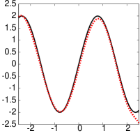
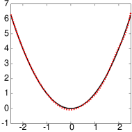
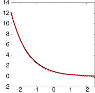
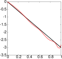
(a) $f_{1}$	(b) $f_{2}$	(c) $f_{3}$	(d) $f_{5}$ in SpAM

Figure 1: Estimated component functions (in dashed red) and true functions (in solid black) for synthetic dataset in Section 5.1. Nonlinear estimates of SPLAM are illustrated in (a) - (c). Figure (d) shows SpAM’s estimate of $f_{5}$. The wiggliness of SpAM’s estimate is because it does not penalize toward exact linearity as does SPLAM.

We plot estimated components in Figure 1. Figure 1 (a), (b), and (c) visualize the nonlinear components in SPLAM for $f_{1}$, $f_{2}$, and $f_{3}$, respectively. We can see that the estimated shape of the component function is very close to the true functions. On this sample, SPLAM perfectly recovers which features are linear and nonlinear while SpAM treats all selected features as nonlinear. For coefficients on linear components in SPLAM, the relative error is less than 0.1%. For comparison, we visualize $f_{5}$ in SpAM in red in Figure 1(d). The ground truth linear function is plotted in black. We can see that the component itself is not exactly linear and that it overfits to the noise.

5.2 Simulation: Effect of $|\mathcal{N}|$ and $|\mathcal{L}|$ on SPLAM, SpAM, and the Lasso

In this section, we perform a large-scale simulation to gain deeper insights into the lasso (Tibshirani, 1996), SPLAM and SpAM (Ravikumar et al., 2009). We consider the models with $p=100$ features: $y=\sum_{j\in\mathcal{L}}x_{j}+\sum_{j\in\mathcal{N}}\sin(x_{j})+\epsilon$, where $\epsilon\sim\mathcal{N}(0,1)$, $\mathcal{L}\cap\mathcal{N}=\emptyset$. We use two parameters $\gamma$ and $\delta$ to control the cardinality of $\mathcal{L}$ and $\mathcal{N}$, respectively, i.e., $|\mathcal{L}|=\gamma p$ and $|\mathcal{N}|=\delta p$. We choose $\gamma=0.0,0.1,...,1.0$ and $\delta=0.0,0.1,...,1.0$ ($\gamma+\delta\leq 1$) and for each $(\gamma,\delta)$ pair, we generate 10 different models. For each of those models, we generate $N_{train}$ points for training, $N_{valid}$ points for validation and $N_{test}$ points for testing. We consider three different settings of simulations, $(N_{train},N_{valid},N_{test})=(200,100,100)$, $(500,100,100),(1000,$ $200,200)$.

For SPLAM, we consider $\alpha\in\{0.05$, $0.1,...,0.95,1\}$. For all of the three methods, we consider the full regularization path with 100 $\lambda$s spaced evenly on a log scale. In our experiments, this range is sufficient to find the optimal model structure. Best model parameters are chosen using the validation set, and model accuracy is evaluated as the average RMSE of 10 models on test sets. For all successive experiments, we use the same method to choose parameters.

	$N_{train}=200$	$N_{train}=500$	$N_{train}=1000$
Nonlinear Terms (%)
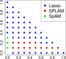
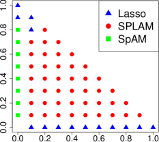
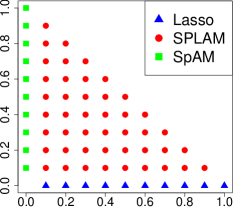
	Linear Terms (%)

Figure 2: Results of simulation in Section 5.2. Each point shows the winning model for a given $(\gamma,\delta)$ pair.

Figure 2 shows the results for the simulations. For each $(\gamma,\delta)$ pair, we plot which model wins on average. It is clear that for pure linear ($\delta=0$) and pure additive ($\gamma=0$), SPLAM has no advantage over the lasso or SpAM.

When $N_{train}=200$, both SpAM and SPLAM overfit significantly when there are a lot of nonlinear components, since a large number of nonlinear components leads to a large parameter space and this small amount of data is not enough for reliable estimates. The lasso wins over the other methods on most of the cases by trading off variance for bias. SPLAM outperforms the lasso in regimes with a mixture of small nonlinear components and a reasonable number of linear components. When we increase the number of data points in the training set ($N_{train}=500$), more reliable estimates can be obtained so SpAM wins back from the lasso on cases where we only have nonlinear components (the lasso, having only linear features is incapable of estimating the nonlinear effects present in the data). Interestingly, the lasso is still the best when there are a lot of nonlinear components since in this regime the data cannot support the large number of parameters for reliable estimation. SPLAM, however, is the winner in most settings since it can better model the mixture of linear and nonlinear effects when there are enough data. Not surprisingly, when there are enough data ($N_{train}=1000$), SPLAM dominates all cases in which both linear and nonlinear components are present. This is because the lasso is unable to model nonlinear effects and because SpAM has higher variance than SPLAM without being less biased.

Table 1: Size (total number of points) and dimension of datasets and performance of methods. For each method, we report the mean error (standard deviation in parentheses) and how many of the selected features are nonlinear, written as $|\hat{\mathcal{N}}|/(|\hat{\mathcal{N}}|+|\hat{\mathcal{L}}|)$. Bold indicates the method with the mean lowest error.

Dataset	Size	Test	$\mathbf{p}$	Lasso		SPLAM		SpAM
Spambase	4601	920	57	7.38 (0.87)	0/52	6.57 (0.91)	38/41	6.93 (0.96)	38/38
Gisette	6000	1200	5000	2.43 (0.54)	0/717	2.18 (0.59)	10/733	2.62 (0.51)	1364/1461
RCV1	697641	418584	47236	2.71 (0.02)	0/7652	2.67 (0.01)	4/5293	3.18 (0.04)	4498/4683
Pantheon	62849	37709	10000	9.34 (0.12)	0/1859	9.22 (0.16)	27/1853	12.71 (0.19)	2770/2770

5.3 Real Problems

In this section, we report experimental results on several real classification problems. We choose datasets with different dimensions and sizes. Table 1 summarizes the characteristics of the datasets and presents the predictive performance of the lasso, SPLAM, and SpAM with means and standard deviations on 5 trials. Best parameters are chosen on a held-out validation set on each trial. We note that SPLAM outperforms the lasso and SpAM on most of the trials. We also list the number of selected nonlinear features and total number of selected features in Table 1. In our experiments, features are forced to be linear if they have less than 10 unique values. This is the case with SpAM on Gisette and RCV1 dataset.

Email Classification. We first consider a classification problem for detecting spam emails (Spambase) (Hastie et al., 2009). The features include statistics of particular words or letters in an email. We see from Table 1 that by allowing features to act nonlinearly, the error of SpAM decreases substantially compared to the lasso. However, by explicitly setting some of the variables to stay linear, SPLAM further outperforms SpAM.

Handwritten Digit Recognition. We use the “Gisette” dataset constructed from NIPS 2003 feature selection challenge (http://www.nipsfsc.ecs.soton.ac.uk/). The problem is to separate the highly confusible digits “4” and “9”. Features in this dataset contain pixels that are necessary to distinguish “4” from “9”, but higher order features from those pixels as well as random noise features are also added. Since the dimension of this dataset is significantly larger than the previous dataset while the size of the dataset remains similar, we expect SpAM to overfit as shown in Table 1. In our experiments, the best SpAM model that we can get is always worse than the lasso on each cross validation set while our SPLAM outperforms the lasso on most cross validation sets. Our SPLAM selects about 733 features, with about 10 of them being nonlinear and the rest being linear, while the lasso selects 717 features. This confirms that by allowing a small number of features to act nonlinearly, we can further improve the classification performance, and yet by setting most of features as linear, we effectively control the complexity and avoid overfitting.

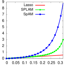
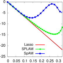
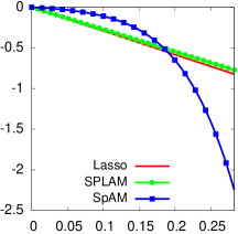
(a)	(b)	(c)

Figure 3: Estimated component functions on RCV1 dataset.

Text Categorization. Text categorization is an important task for many natural language processing applications. We use Reuters Corpus Volume I (RCV1) which involves binary classification (Lewis et al., 2004). From Table 1 we see that SPLAM outperforms the others. This suggests that in high dimensions, there is extra accuracy that can be obtained over the lasso if some features are allowed to be nonlinearly transformed. However, if all features are allowed to be nonlinearly transformed, such as in SpAM, the model will overfit and a suboptimal model is obtained. On average SPLAM selects 5293 features with 4 of them being nonlinear, and the lasso selects 7652 features. Figure 3 visualizes some components in SPLAM, SpAM, and the lasso. Each feature in this dataset relates to the (normalized) frequency of some word in a document. In general, we find that SPLAM strikes a compromise between the lasso and SpAM fits, using nonlinearity only sparingly. Figure 3 (a) shows a feature which is identified as nonlinear by both SPLAM and SpAM. Notice that both SPLAM and SpAM find a model with similar shape. In Figure 3 (b), we show a feature that appears to be nearly linear in SPLAM. In this case, SpAM oscillates in a way that might suggest that it is overfitting to the noise; by contrast, SPLAM’s fit is mostly linear, only exhibiting nonlinear effects when the input gets large. Notice SPLAM and the lasso almost agree with each other when the feature value is small. Finally, in Figure 3 (c) we show a feature that is linear in both SPLAM and the lasso. SPLAM’s estimation of the slope is very similar to that of the lasso. By contrast, SpAM treats this as a nonlinear effect. In light of SPLAM’s better misclassification rate in this data set, one might suppose that SpAM’s more pronounced deviations from linearity are in fact cases of overfitting to noise. Likewise, SPLAM’s better misclassification rate compared to the lasso suggests that the latter may be failing to model some of the nonlinear effects.

Image Matching. Many new computer vision applications are utilizing large-scale datasets of places derived from the many billions of photos on the Web. Image matching is a central procedure to those applications which tests whether two images are geometrically consistent (Lou et al., 2012). Since image matching is an expensive procedure, image pairs are usually pre-filtered with a lightweight classification procedure to estimate whether two images are likely to pass the geometric verification. In this study, we use the “Pantheon” dataset in Lou et al. (2012). Each image is represented using bag-of-visual-words model with a vocabulary of 10,000 visual words. From Table 1 we again observe that by carefully controlling the complexity of the model, SPLAM has better predictive performance than the other two models. On average the lasso selects 1859 features while SPLAM selects 1853 features with only 27 of them being nonlinear.

6 Conclusion

In this paper, we introduce the sparse partially linear additive model that performs two model-selection tasks within a single convex hierarchical sparse regularization problem. This formulation permits an efficient optimization algorithm, making the GPLAM framework practical in machine learning settings. We develop an oracle inequality of SPLAM that makes no assumptions on the design matrix, and we study SPLAM’s advantage over SpAM when many of the features in the model are linear. Our thorough experiments demonstrate that SPLAM can effectively and accurately find relevant components with proper complexity and is very competitive for additive modeling. In particular, on large-scale, high-dimensional datasets, SPLAM improves accuracy over the popular linear model by allowing a small set of features to have a nonlinear effect.

7 Acknowledgments

The authors gratefully acknowledge Johannes Lederer for useful discussions. This research has been supported by the NSF under Grants IIS-0911036 and IIS-1012593.

Appendix A Convergence of Algorithm 1 in the Main Paper

We show that Algorithm 1 fits the general BCGD framework (Tseng and Yun, 2009) and therefore the global convergence is guaranteed. We include this supplementary material for completeness although a similar convergence result for the group lasso is shown in Qin et al. (2010). We first briefly review the general BCGD algorithm.

Let $F(\beta)=L(\beta)+h(\beta)$, where $h(\beta)=\lambda\Omega^{{SPLAM}}(\beta)$. At each iteration $k$, for block $j$, choose a symmetric positive definite matrix $H^{k}$, and compute the search direction.

$$d^{k}=\arg\min_{d}\{\nabla L(\beta^{k})^{T}d+\frac{1}{2}d^{T}H^{k}d+h(\beta^{k}+d)\}$$ (13)

where $\forall i\not\in\mathcal{G}_{j},d_{i}=0$. Then a step size $\alpha^{k}>0$ is chosen so that the following Armijo rule is satisfied,

$$F(\beta^{k}+\alpha^{k}d^{k})\leq F(\beta^{k})+\alpha^{k}\sigma\Delta^{k}$$ (14)

where $0<\sigma<1,0\leq\gamma<1$, and

$$\Delta^{k}\overset{\text{def}}{=}\nabla L(\beta^{k})^{T}d^{k}+\gamma{d^{k}}^{T}H^{k}d^{d}+h(\beta^{k}+d^{k})-h(\beta^{k}),$$ (15)

Once the step size $\alpha^{k}$ is determined, update $\beta^{k+1}=\beta^{k}+\alpha^{k}d^{k}$.

Theorem 2 in Tseng and Yun (2009) guarantees the global convergence when $\overline{\theta}I\succeq H^{k}\succeq\underline{\theta}I$, $0<\underline{\theta}\leq\overline{\theta}$.

Theorem 2.

Algorithm 1 fits the general BCGD framework of Tseng and Yun (2009). The global convergence is guaranteed and Algorithm 1 converges Q-linearly.

Proof.

First, for block $j$, setting $H^{k}=\frac{1}{t_{j}}I$, Equation (13) is equivalent to our proximal operator for block $j$ after ignoring constants. Next, notice that when $\alpha^{k}=1,\sigma=1$, and $\gamma=\frac{1}{2}$, the Armijo rule becomes our backtracking line search step in Equation (8) in the main paper. That is, the effort of choosing step size is shifted to finding $H^{k}$. Besides, Lemma 1 in Tseng and Yun (2009) suggests $\nabla L(\beta^{k})^{T}d^{k}+{d^{k}}^{T}H^{k}d^{k}+h(\beta^{k}+d^{k})-h(\beta^{k})\leq 0$. Since $H^{k}\succ 0$, with $\gamma=\frac{1}{2}$, we can easily see $\Delta^{k}\leq 0$ whenever $d^{k}\neq 0$, which means if the Armijo rule holds for $\sigma=1$, it must also hold for $\sigma<1$. Finally, we show that $\overline{\theta}I\succeq H^{k}\succeq\underline{\theta}I$. Assume the initial step size is $t_{j}^{0}$, this is true when $\overline{\theta}=\max\{C_{j},1/t_{j}^{0}\}$ and $\underline{\theta}=\min\{C_{j},1/t_{j}^{0}\}$. Thus, according to Theorem 2 in Tseng and Yun (2009), Algorithm 1 converges Q-linearly. ∎

Appendix B Practical Issues

B.1 Active Set Strategy

We employ the widely used active set strategy (Friedman et al., 2010; Krishnapuram et al., 2005; Meier et al., 2008). After a complete cycle through all the variables, we iterate only on the active set till convergence. If another complete cycle does not change the active set, we are done, otherwise the process is repeated.

B.2 Regularization Path

Similar to glmnet (Friedman et al., 2010), the optimization of SPLAM also uses two parameters, $\lambda$ and $\alpha$, which usually involves a grid search on values of $(\lambda,\alpha)$ pairs. As noted in the main paper, for each value of $\alpha$, we start at the smallest value $\lambda_{max}$ for which $\beta_{j}=0$ for $j=1,...,p$. We then decrease $\lambda$ from $\lambda_{max}$ exponentially. To find $\lambda_{max}$, we note that for all $\lambda\geq\lambda_{init}=\max_{j}\frac{\|\nabla_{\beta_{j}}L(0)\|_{2}}{\alpha}$, the zero vector is the solution to our optimization problem. We perform a binary search to find $\lambda_{max}$. As described in Algorithm 3, we start with $\lambda_{init}$ (Line 1) and effectively shrink the interval $[\lambda_{l},\lambda_{h}]$ (Line 3 - 8) to locate $\lambda_{max}$.

Algorithm 3 Finding $\lambda_{max}$

1:  $\lambda_{h}\leftarrow\max_{j}\frac{\|\nabla_{j}L(0)\|_{2}}{\alpha}$

2:  $\lambda_{l}\leftarrow 0$

3:  while $\lambda_{h}-\lambda_{l}\geq\epsilon$ do

4:     $\lambda\leftarrow\frac{\lambda_{h}+\lambda_{l}}{2}$

5:     if $\forall j,P_{t}^{j}(0)=0$ then

6:        $\lambda_{h}\leftarrow\lambda$

7:     else

8:        $\lambda_{l}\leftarrow\lambda$

9:  $\lambda_{max}=\lambda_{h}$

Appendix C Proof of Theorem 1 and Corollary 1 in the Main Paper

Proof of Theorem 1.

By definition of $\hat{\beta}$,

$$\frac{1}{2N}\|y-X\hat{\beta}\|_{2}^{2}+\lambda\Omega^{{SPLAM}}(\hat{\beta})\leq\frac{1}{2N}\|y-X\beta\|_{2}^{2}+\lambda\Omega^{{SPLAM}}(\beta)$$

holds for any $\beta\in\mathbb{R}^{p}$. Some algebra (recalling that $y=f^{0}+\epsilon$ and writing $\hat{\Delta}=\hat{\beta}-\beta$) leads to

$$\frac{1}{2N}\|X\hat{\beta}-f^{0}\|_{2}^{2}+\lambda\Omega^{{SPLAM}}(\hat{\beta})\leq\frac{1}{2N}\|X\beta-f^{0}\|_{2}^{2}+\frac{1}{N}\epsilon^{T}X\hat{\Delta}+\lambda\Omega^{{SPLAM}}(\beta)$$ (16)

Define the empirical process as,

$$V_{N}(\hat{\Delta})=\frac{1}{N}\epsilon^{T}X\hat{\Delta}=\frac{1}{\sqrt{N}}\sum_{j=1}^{p}V_{j}^{T}\hat{\Delta}_{j}$$ (17)

where $V_{j}=\frac{1}{\sqrt{N}}X_{j}^{T}\epsilon\in\mathbb{R}^{M}$.

Now we bound the empirical process. First we notice that,

$$|V_{j}^{T}\hat{\Delta}_{j}|\leq \frac{1}{2}\left[|V_{j}^{T}\hat{\Delta}_{j}|+|V_{j1}\hat{\Delta}_{j1}|+|V_{j,-1}^{T}\hat{\Delta}_{j,-1}|\right]$$ (18)

$$\leq \frac{1}{2}\left[\|V_{j}\|_{2}\|\hat{\Delta}_{j}\|_{2}+|V_{j1}||\hat{\Delta}_{j1}|+\|V_{j,-1}\|_{2}\|\hat{\Delta}_{j,-1}\|_{2}\right]$$ (19)

Thus $|V_{N}(\hat{\Delta})|$ can be bounded as follows.

$$|V_{N}(\hat{\Delta})|\leq \frac{1}{\sqrt{N}}\sum_{j=1}^{p}|V_{j}^{T}\hat{\Delta}_{j}|$$ (20)

$$\leq \frac{1}{2\sqrt{N}}\left(\max_{j}\|V_{j}\|_{2}\|\hat{\Delta}\|_{2,1}+\max_{j}|V_{j1}|\sum_{j}|\hat{\Delta}_{j1}|+\max_{j}\|V_{j,-1}\|_{2}\|\hat{\Delta}_{\cdot,-1}\|_{2,1}\right)$$ (21)

$$\leq \frac{1}{2\sqrt{N}}\left[(\max_{j}\|V_{j}\|_{2}+\max_{j}|V_{j1}|)\|\hat{\Delta}\|_{2,1}+\max_{j}\|V_{j,-1}\|_{2}\|\hat{\Delta}_{\cdot,-1}\|_{2,1}\right]$$ (22)

Observing that $V_{j}\sim N(0,\sigma^{2}I_{M})$, we have $\|V_{j}\|_{2}^{2}\sim\sigma^{2}\chi^{2}_{M}$. Thus, by Lemma 6.2 and 8.1 of Bühlmann and van de Geer (2011), we have

$$P\left(\frac{\max_{j}|V_{j1}|}{2\sqrt{N}}>\nu_{1}\right)\leq 2e^{-x}$$ (23)

$$P\left(\frac{\max_{j}\|V_{j}\|_{2}}{2\sqrt{N}}>\nu_{2}\right)\leq e^{-x}$$ (24)

where,

$$\nu_{1}^{2}= \frac{\sigma^{2}}{2N}(x+\log p)$$ (26)

$$\nu_{2}^{2}= \frac{\sigma^{2}}{4N}\left[M+\sqrt{4M(x+\log p)}+4(x+\log p)\right]$$ (27)

Thus, we have

$$P\left(\frac{\max_{j}\|V_{j}\|_{2}+\max_{j}|V_{j1}|}{2\sqrt{N}}>\nu_{1}+\nu_{2}\right)\leq 3e^{-x}$$ (28)

$$P\left(\frac{\max_{j}\|V_{j,-1}\|_{2}}{2\sqrt{N}}>\nu_{2}\right)\leq e^{-x}$$ (29)

Therefore (with union bound),

$$P\left(|V_{N}(\hat{\Delta})|\leq\left[(\nu_{1}+\nu_{2})\|\hat{\Delta}\|_{2,1}+\nu_{2}\|\hat{\Delta}_{\cdot,-1}\|_{2,1}\right]\right)\geq 1-(e^{-x}+3e^{-x})$$ (30)

$$= 1-4e^{-x}$$ (31)

Thus, by (16) we have with probability at least $1-4e^{-x}$ that

$$\frac{1}{2N}\|X\hat{\beta}-f^{0}\|_{2}^{2}+\lambda\Omega^{{SPLAM}}(\hat{\beta})\leq\frac{1}{2N}\|X\beta-f^{0}\|_{2}^{2}+(\nu_{1}+\nu_{2})\|\hat{\Delta}\|_{2,1}+\nu_{2}\|\hat{\Delta}_{\cdot,-1}\|_{2,1}+\lambda\Omega^{{SPLAM}}(\beta)$$ (32)

Let $\lambda_{1}=\lambda\alpha$ and $\lambda_{2}=\lambda(1-\alpha)$, we can take $\lambda_{1}=2(\nu_{1}+\nu_{2})$ and $\lambda_{2}=2\nu_{2}$. Thus, (32) implies

$$\frac{1}{2N}\|X\hat{\beta}-f^{0}\|_{2}^{2} -\frac{1}{2N}\|X\beta-f^{0}\|_{2}^{2}\leq(\lambda/2)\Omega^{{SPLAM}}(\hat{\Delta})-\lambda\Omega^{{SPLAM}}(\hat{\beta})+\lambda\Omega^{{SPLAM}}(\beta)$$ (33)

$$\leq (\lambda/2)\left[\Omega^{{SPLAM}}(\hat{\beta})+\Omega^{{SPLAM}}(\beta)\right]-\lambda\Omega^{{SPLAM}}(\hat{\beta})+\lambda\Omega^{{SPLAM}}(\beta)$$ (34)

$$= (3\lambda/2)\Omega^{{SPLAM}}(\beta)-(\lambda/2)\Omega^{{SPLAM}}(\hat{\beta})$$ (35)

by the triangle inequality. Thus,

$$\frac{1}{2N}\|X\hat{\beta}-f^{0}\|_{2}^{2}\leq\frac{1}{2N}\|X\beta-f^{0}\|_{2}^{2}+3\lambda\Omega^{{SPLAM}}(\beta).$$ (36)

By choosing $x=\log p$, we can ensure our inequality holds with probability at least $1-4/p$. This means,

$$\nu_{1}^{2}= \frac{\sigma^{2}}{N}\log p$$ (37)

$$\nu_{2}^{2}= \frac{\sigma^{2}}{4N}\left[M+\sqrt{8M\log p}+8\log p\right].$$ (38)

Define $\tilde{\nu}_{1}^{2}\overset{\text{def}}{=}\frac{\sigma^{2}}{N}\log p$ and notice that $\nu_{2}^{2}\leq 6\sigma^{2}\log p/N\overset{\text{def}}{=}\tilde{\nu}_{2}^{2}$ if $\log p\geq M/8$. Now, as long as $\log p\geq M/8$, we can take $\lambda\geq 2(\tilde{\nu}_{1}+2\tilde{\nu}_{2})=2(1+2\sqrt{6})\sigma\sqrt{\log p/N}$ and

$$\alpha=\frac{\tilde{\nu}_{1}+\tilde{\nu}_{2}}{\tilde{\nu}_{1}+2\tilde{\nu}_{2}}=\frac{1+\sqrt{6}}{1+2\sqrt{6}},$$ (39)

with probability at least $1-4/p$, we have

$$\frac{1}{2N}\|X\hat{\beta}-f^{0}\|_{2}^{2}\leq\frac{1}{2N}\|X\beta-f^{0}\|_{2}^{2}+3\lambda\Omega^{{SPLAM}}(\beta).$$ (40)

This holds simultaneously for all $\beta$; this may be succinctly expressed by adding $\min_{\beta}$ to the right hand side.

∎

Proof of Corollary 1.

We plug $\beta^{0}$ into the right-hand side of Theorem 1 and observe that

$$\Omega^{{SPLAM}}(\beta^{0}) =\alpha\sum_{j\in\mathcal{S}^{0}}\|\beta^{0}_{j}\|_{2}+(1-\alpha)\sum_{j\in\mathcal{N}^{0}}\|\beta_{j,-1}^{0}\|_{2}$$ (41)

$$\leq\alpha\sum_{j\in\mathcal{L}^{0}}\|\beta^{0}_{j}\|_{2}+\sum_{j\in\mathcal{N}^{0}}\|\beta_{j}^{0}\|_{2}$$ (42)

$$=\alpha\sum_{j\in\mathcal{L}^{0}}|\beta^{0}_{j1}|+\sum_{j\in\mathcal{N}^{0}}\|\beta_{j}^{0}\|_{2}$$ (43)

∎

Appendix D Proof of Lower Bound on SpAM’s Prediction Error

We assume that all $p$ features are linear with equal coefficients, i.e., $\beta_{j}^{0}=be_{1}\in\mathbb{R}^{M}$ and consider an asymptotic regime in which $p$ is fixed and $N=pM$, with $M,N\to\infty$. We assume that all features are orthogonal, i.e., $\frac{1}{N}X^{T}X=I_{pM}$. In the main paper, we note that SpAM in this case is given by the expression:

$$\hat{\beta}_{j}^{{SpAM}}=\gamma_{j}(\lambda)\frac{1}{N}X_{j}^{T}y\quad\text{where}\quad\gamma_{j}(\lambda)=\left(1-\frac{\lambda}{\|\frac{1}{N}X_{j}^{T}y\|_{2}}\right)_{+}.$$

Now, $\frac{1}{N}X_{j}^{T}y=be_{1}+U_{j}$ where $U_{j}=\frac{1}{N}X_{j}^{T}\epsilon\sim N(0,\frac{\sigma^{2}}{N}I_{M})$. Since $\|\frac{1}{N}X_{j}^{T}y\|_{2}^{2}\to b^{2}+\sigma^{2}/p$, asymptotically, the shrinkage factor $\gamma_{j}(\lambda)=\gamma$ is a nonrandom value, not depending on $j$, and the prediction error is

$$\frac{1}{N}\|X\hat{\beta}^{{SpAM}}-X\beta^{0}\|^{2} =\sum_{j=1}^{p}\|\gamma(be_{1}+U_{j})-be_{1}\|^{2}$$

$$=\gamma^{2}(b^{2}p+\sum_{j=1}^{p}\left[\|U_{j}\|^{2}+2bU_{j1}\right])+pb^{2}-2\gamma\sum_{j=1}^{p}b(b+U_{j1})$$

$$\to\gamma^{2}(b^{2}p+\sigma^{2})+pb^{2}-2\gamma pb^{2}.$$

For the best possible asymptotic error, we can choose $\gamma=pb^{2}/(pb^{2}+\sigma^{2})$ (equivalent to choosing the best $\lambda$). At this value,

$$\lim_{N\to\infty}\frac{1}{N}\|X\hat{\beta}^{{SpAM}}-X\beta^{0}\|^{2}\geq\frac{b^{2}}{1/b^{2}+p/\sigma^{2}}>0.$$

Thus, SpAM is not consistent in terms of prediction error in this asymptotic regime.

To see that SPLAM with $\lambda\alpha=0$ and $\lambda(1-\alpha)=\infty$ is consistent in terms of prediction error, observe that $\hat{\beta}^{{SPLAM}}=(X_{j1}^{T}y)e_{1}=(b+U_{j1})e_{1}$ and

$$\frac{1}{N}\|X\hat{\beta}^{{SPLAM}}-X\beta^{0}\|^{2}=\sum_{j=1}^{p}\|(b+U_{j1})e_{1}-be_{1}\|^{2}=\sum_{j=1}^{p}U_{j1}^{2}\sim\frac{\sigma^{2}}{N}\chi^{2}_{p}\to 0.$$

Appendix E Experiments

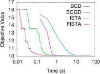
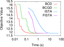
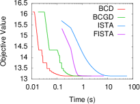
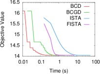
(a) $\lambda=0.01,\alpha=0.1$	(b) $\lambda=0.01,\alpha=0.15$	(c) $\lambda=0.01,\alpha=0.2$	(d) $\lambda=0.01,\alpha=0.25$
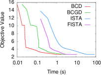
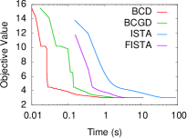
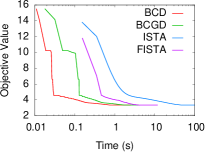
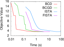
(e) $\lambda=0.001,\alpha=0.1$	(f) $\lambda=0.001,\alpha=0.15$	(g) $\lambda=0.001,\alpha=0.2$	(h) $\lambda=0.001,\alpha=0.25$

Figure 4: Objective value vs. running time for synthetic dataset in Section 5.1.

In this section, we compare our BCGD algorithm and BCD algorithm with ISTA and FISTA (Beck and Teboulle, 2009) using the synthetic function in Section 5.1. We report running time of all the methods on a single core. For BCGD, ISTA, and FISTA, we start with a same initial step size. For fair comparison, we turn off the active set strategy in BCGD and BCD, and we directly use the design matrix after QR decomposition so that all methods are applied to the same optimization problem.

Figure 4 illustrates the running time for all methods using the same synthetic dataset in Section 5.1 for different combinations of $\lambda$ and $\alpha$. As expected, FISTA converges much faster than ISTA. However, the BCGD algorithm is faster than both of the these methods. This is because BCGD uses more information in the sense of more frequent updates. In addition, we can see that BCD further speeds up the optimization since there is no step size in BCD; this not only solves exactly the subproblem but also avoids the possibility of dampening the step size and repeating the computation on the same block.

References

- Beck and Teboulle (2009) Beck, A. and Teboulle, M. (2009). A fast iterative shrinkage-thresholding algorithm for linear inverse problems. SIAM Journal on Imaging Sciences, 2(1), 183–202.
- Bühlmann and van de Geer (2011) Bühlmann, P. and van de Geer, S. (2011). Statistics for high-dimensional data: methods, theory and applications. Springer, Berlin, Heidelberg.
- Bunea (2004) Bunea, F. (2004). Consistent covariate selection and post model selection inference in semiparametric regression. The Annals of Statistics, 32(3), 898–927.
- Candès and Plan (2009) Candès, E. and Plan, Y. (2009). Near-ideal model selection by minimization. The Annals of Statistics, 37(5A), 2145–2177.
- Candes and Tao (2007) Candes, E. and Tao, T. (2007). The dantzig selector: Statistical estimation when p is much larger than n. The Annals of Statistics, 35(6), 2313–2351.
- Chatterjee et al. (2012) Chatterjee, S., Steinhaeuser, K., Banerjee, A., Chatterjee, S., and Ganguly, A. (2012). Sparse group lasso: Consistency and climate applications. In SDM, pages 47–58.
- Chen et al. (2011) Chen, R., Liang, H., and Wang, J. (2011). Determination of linear components in additive models. Journal of Nonparametric Statistics, 23(2), 367–383.
- Chouldechova and Hastie (2015) Chouldechova, A. and Hastie, T. (2015). Generalized additive model selection. arXiv preprint arXiv:1506.03850.
- Dalalyan et al. (2014) Dalalyan, A., Hebiri, M., and Lederer, J. (2014). On the prediction performance of the lasso. arXiv preprint arXiv:1402.1700.
- Dinse and Lagakos (1983) Dinse, G. and Lagakos, S. (1983). Regression analysis of tumour prevalence data. Applied Statistics, 32(3), 236–248.
- Du et al. (2012) Du, P., Cheng, G., and Liang, H. (2012). Semiparametric regression models with additive nonparametric components and high dimensional parametric components. Computational Statistics & Data Analysis, 56(6), 2006–2017.
- Engle et al. (1986) Engle, R., Granger, C., Rice, J., and Weiss, A. (1986). Semiparametric estimates of the relation between weather and electricity sales. Journal of the American Statistical Association, 81(394), 310–320.
- Friedman et al. (2010) Friedman, J., Hastie, T., and Tibshirani, R. (2010). Regularization paths for generalized linear models via coordinate descent. Journal of Statistical Software, 33(1), 1.
- Green and Silverman (1993) Green, P. and Silverman, B. (1993). Nonparametric regression and generalized linear models: a roughness penalty approach. CRC Press.
- Härdle and Liang (2007) Härdle, W. and Liang, H. (2007). Partially linear models. Springer.
- Hastie and Tibshirani (1990) Hastie, T. and Tibshirani, R. (1990). Generalized additive models. Chapman & Hall/CRC.
- Hastie et al. (2009) Hastie, T., Tibshirani, R., and Friedman, J. (2009). The elements of statistical learning (2nd edition). Springer New York.
- Hebiri and Lederer (2013) Hebiri, M. and Lederer, J. (2013). How correlations influence lasso prediction. IEEE Transactions on Information Theory, 59(3), 1846–1854.
- Huang et al. (2012) Huang, J., Wei, F., and Ma, S. (2012). Semiparametric regression pursuit. Statistica Sinica, 22(4), 1403–1426.
- Jenatton et al. (2010) Jenatton, R., Mairal, J., Bach, F., and Obozinski, G. (2010). Proximal methods for sparse hierarchical dictionary learning. In ICML, pages 487–494.
- Krishnapuram et al. (2005) Krishnapuram, B., Carin, L., Figueiredo, M., and Hartemink, A. (2005). Sparse multinomial logistic regression: Fast algorithms and generalization bounds. Transactions on Pattern Analysis and Machine Intelligence, 27(6), 957–968.
- Lewis et al. (2004) Lewis, D., Yang, Y., Rose, T., and Li, F. (2004). Rcv1: A new benchmark collection for text categorization research. The Journal of Machine Learning Research, 5, 361–397.
- Lian and Liang (2013) Lian, H. and Liang, H. (2013). Generalized additive partial linear models with high-dimensional covariates. Econometric Theory, 29, 1136–1161.
- Lian et al. (2012) Lian, H., Chen, X., and Yang, J. (2012). Identification of partially linear structure in additive models with an application to gene expression prediction from sequences. Biometrics, 68(2), 437–445.
- Lin and Zhang (2006) Lin, Y. and Zhang, H. (2006). Component selection and smoothing in multivariate nonparametric regression. The Annals of Statistics, 34(5), 2272–2297.
- Lou et al. (2012) Lou, Y., Snavely, N., and Gehrke, J. (2012). Matchminer: Efficient spanning structure mining in large image collections. In ECCV.
- Meier et al. (2008) Meier, L., van de Geer, S., and Bühlmann, P. (2008). The group lasso for logistic regression. Journal of the Royal Statistical Society: Series B (Statistical Methodology), 70(1), 53–71.
- Müller and van de Geer (2013) Müller, P. and van de Geer, S. (2013). The partial linear model in high dimensions. arXiv preprint arXiv:1307.1067.
- Negahban et al. (2012) Negahban, S., Ravikumar, P., Wainwright, M., and Yu, B. (2012). A unified framework for high-dimensional analysis of -estimators with decomposable regularizers. Statistical Science, 27(4), 538–557.
- Nelder and Wedderburn (1972) Nelder, J. A. and Wedderburn, R. W. M. (1972). Generalized linear models. Journal of the Royal Statistical Society. Series A (General), 135(3), 370–384.
- Obozinski et al. (2011) Obozinski, G., Jacob, L., and Vert, J.-P. (2011). Group lasso with overlaps: the latent group lasso approach. arXiv preprint arXiv:1110.0413.
- Petersen et al. (2014) Petersen, A., Witten, D., and Simon, N. (2014). Fused Lasso Additive Model. ArXiv e-prints.
- Qin et al. (2010) Qin, Z., Scheinberg, K., and Goldfarb, D. (2010). Efficient block-coordinate descent algorithms for the group lasso. Mathematical Programming Computation, pages 1–27.
- Ravikumar et al. (2009) Ravikumar, P., Liu, H., Lafferty, J., and Wasserman, L. (2009). Sparse additive models. Journal of the Royal Statistical Society: Series B (Statistical Methodology), 71(5), 1009–1030.
- Rigollet and Tsybakov (2011) Rigollet, P. and Tsybakov, A. (2011). Exponential screening and optimal rates of sparse estimation. The Annals of Statistics, 39(2), 731–771.
- Tibshirani (1996) Tibshirani, R. (1996). Regression shrinkage and selection via the lasso. Journal of the Royal Statistical Society. Series B (Methodological), pages 267–288.
- Tseng and Yun (2009) Tseng, P. and Yun, S. (2009). A coordinate gradient descent method for nonsmooth separable minimization. Mathematical Programming, 117(1-2), 387–423.
- van de Geer (2007) van de Geer, S. (2007). The deterministic lasso. In JSM.
- van de Geer and Bühlmann (2009) van de Geer, S. and Bühlmann, P. (2009). On the conditions used to prove oracle results for the lasso. Electronic Journal of Statistics, 3, 1360–1392.
- Wang et al. (2014) Wang, L., Xue, L., Qu, A., and Liang, H. (2014). Estimation and model selection in generalized additive partial linear models for correlated data with diverging number of covariates. The Annals of Statistics, 42(2), 592–624.
- Xie and Huang (2009) Xie, H. and Huang, J. (2009). Scad-penalized regression in high-dimensional partially linear models. The Annals of Statistics, 37(2), 673–696.
- Zhang et al. (2011) Zhang, H., Cheng, G., and Liu, Y. (2011). Linear or nonlinear? automatic structure discovery for partially linear models. Journal of the American Statistical Association, 106(495).
- Zhao et al. (2009) Zhao, P., Rocha, G., and Yu, B. (2009). The composite absolute penalties family for grouped and hierarchical variable selection. The Annals of Statistics, 37(6A), 3468–3497.