Population aging through survival of the fit and stable

Abstract

Motivated by the wide range of known self-replicating systems, some far from genetics, we study a system composed by individuals having an internal dynamics with many possible states that are partially stable, with varying mutation rates. Individuals reproduce and die with a rate that is a property of each state, not necessarily related to its stability, and the offspring is born on the parent’s state. The total population is limited by resources or space, as for example in a chemostat or a Petri dish. Our aim is to show that mutation rate and fitness become more correlated, even if they are completely uncorrelated for an isolated individual, underlining the fact that the interaction induced by limitation of resources is by itself efficient for generating collective effects.

This work concerns the population dynamics of a system of self-replicating individuals, with complex internal dynamics, where the state of the system is not necessarily characterized by a genum, but could also be the transcriptional situation. A variety of scenarios of self-replication have recently attracted considerable attention. These include models of prebiotic evolution segre_prebiotic , cells subjected to unforeseen challenges braun , and artificial self-replication and evolution artificial_self_rep . In all these cases, the complex dynamics might give rise to a wide spectrum of replication cycle stabilities, implying ‘mutation rates’ that show large variability (here and in what follows ‘mutation rate’ will be used to denote changes even in non-genetic contexts). In fact, genetic mutation rates themselves may vary by many orders of magnitude Saunders_phase_variation , and epigenetic changes occur at yet another set of time-scales Schmitz_epigenetic_rate . Moreover, in systems that have not yet undergone a long process of evolution, mutation rates might not be much smaller than growth rates.

The purpose of this paper is to study the effect that the spread of mutation rates has on the population development, through its interplay with fitness of the individuals, and to do so in a setting which assumes as little as possible about the individuals’ internal structure. Given the wide range of disparate systems which are able to self-replicate and subsequently evolve, it is natural to ask what phenomena will be common to many of them. A ‘null model’ for such a general situation should include as little as possible of details of the systems’ phase-space (‘phenotypes’) and dynamics. For example, we wish to exclude effects of long memory of the state in a single individual after many mutations, which may be highly relevant for genetics, and indeed lead to effects such as genetic ‘hitchhiking’ effects, or to the length of adaptive walks, where an individual wanders on a given landscape adaptive_walks . In genetics, mutation rates are often low compared to growth rates, and can often be taken to be constant or assumed to have a small number of values. In contrast, the stability of a dynamical self-replication state (interpreted as an inverse mutation rate) may vary significantly between states, and cannot be taken a-priori as much lower than growth rates.

To model the individuals’ dynamics, trap models Bouchaud have been extensively used to give simple descriptions to highly complex systems, including relaxation of glasses and rehology of soft and biological materials trap_application1 ; trap_application2 . Trap models have no memory of the state after leaving it, and the new state is chosen at random. The model is therefore fully characterized by the distribution of trap ‘stabilities’, the average times spent in a given trap. By considering a population of systems with can also self-replicate, the resulting model belongs to the house-of-cards class of models Kingman ; Krug ; Krug1 , but with a large dispersion of mutation rates. The existence of multiple mutation rates has been studied in the past Leigh ; Ishii ; Taddei ; Lynch . We are interested here specifically in the phenomena derived from the combination of (i) a large number possible states (as one may envision in a cellular system with more than a few phenotypic switches) and (ii) a large dispersion in the mutation rates. Individuals interact only via some constraint on the total population size, due to limitations such as space or nutrients. Some of our results are, as we shall see, remarkably insensitive to details.

Internal dynamics, selection.

We shall assume that the system has $M(t)$ individuals, with an internal dynamics that has states or attractors (for example a ‘cell fate’) labeled ‘a’ that are not fully stable, mutations are random with probability per unit time $\mu_{a}$. Being in a state a confers an individual a rate of reproduction, or ‘fitness’ $\lambda_{a}$ per unit time. Therefore, each individual is characterized by a pair of numbers $\left(\lambda,\mu\right)$. The dynamics is as follows: when an individual leaves a state $\left(\lambda_{1},\mu_{1}\right)$, it may fall on another state $(\lambda,\mu)$ with probability $p(\lambda,\mu)$, which defines the distribution of states, and is independent of $\left(\lambda_{1},\mu_{1}\right)$ . After a replication, which is asexual, the two daughters inherit the state of the parent. We will work in the limit where the number of attractors $N$ is very large, so that the chances of falling twice in the same one are negligible. This means that within this model if two individuals have exactly the same $(\lambda,\mu)$, they are in the same state as their common ancestor and have never mutated. This model may be viewed as a ‘House of Cards’ model with variable mutation rates Kingman ; Krug ; Krug1 . Alternatively, it is a ‘trap model’ Bouchaud with added self-replication.

Reproduction rates cannot be arbitrarily large because of physical constraints, so the distribution must be bounded, $\lambda<\lambda_{max}$. On the contrary, mutational timescales $1/\mu$ might be quite large, as one may conceive that, for example, some phenotypic ‘cell fates’ may be very stable. We shall thus consider $\mu>\mu_{min}$, where $\mu_{min}\geq 0$ is always small, even zero. Although mutations and fitness may be directly correlated, it is instructive and simpler on a first approach to consider them independent; especially because one of the main purposes of this paper is to pinpoint the correlations that develop in a population but are absent for a single individual. We shall thus choose a product form

$$p(\lambda,\mu)\propto Q(\lambda)P(\mu)$$ (1)

$P(\mu)$ is defined for $\mu>\mu_{min}$, which we shall often take as $0$. For small $\mu$ we shall consider below a power law ($P\sim\mu^{\alpha}$), and more rapidly decaying distributions $P\sim e^{-\mu^{-n}}$ trap_model_comment . We shall assume the distribution of $\lambda$ falls to zero above some $\lambda_{max}$, as $Q(\lambda)\sim(\lambda_{max}-\lambda)^{r}$, with $\lambda\geq 0$. The independence of the distributions corresponds to the assumption of absence of a mechanism tailored to tune mutation rates of an individual according to the external conditions. Another possibility we could have considered is that the independent variables are $\lambda$ and $\hat{\mu}\equiv\lambda/\mu$:

$$\hat{p}(\lambda,\hat{\mu})\propto Q(\lambda)\bar{P}(\hat{\mu})$$ (2)

In order to complete the definition, it is natural to assume that some mechanism, such as the total amount of food or space, constrains the population. In both cases, our conclusion will be that a priori uncorrelated fitness and mutation rates become correlated through natural selection.

I Well-Mixed System

Let us first consider a well-mixed situation, such as a chemostat. Individuals compete for resources which limit their growth rate, and also die or are removed from the system. Here we adopt the standard Moran process, where population size is kept constant by removing an individual at random every time a replication occurs.

Starting from a population in a bounded distribution of $\lambda$ and $\mu$, it turns out one can distinguish four stages in the evolution, see Fig. 1: (I) a continuous stage in which the population of all states is a negligible fraction of the total, (II) a condensation stage in which a significant fraction of the population concentrates in a small range of values of ‘genetic load’ $L$ defined as

$$L\equiv\mu-\lambda\,.$$ (3)

This leads to a (III) takeover phase characterized by rare and rapid changes of single dominant states holding a finite fraction of the population. These takeovers become statistically rarer as time passes. This is analogous, for the well-mixed system, to the ‘Successional Mutation Regime’ of Ref. Fisher1 . Finally, there comes a time when the average time between takeovers stabilizes because the system has optimized as much as it can, this is the beginning of (IV) saturation stage. The population may, of course, start at one of the later stages, and continue its evolution from there.

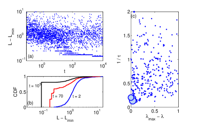
Figure 1: (a) Population evolution in time, stages (I)-(III), for $P\left(\mu\right)=\mu^{-2}e^{-1/\mu}$ and $M=1000$. Points are $L$-values of individuals. For clarity 1 in 40 individuals is plotted. (b) Cumulative distribution function (CDF) of L-values, at $t=2,70,10^{5}$. (c) Distribution of states in the $\left(\lambda,\mu\right)$-plane at $t=70$. Circle sizes indicate the number of individuals in a state. Large clusters have low $\mu$ and high $\lambda$, the continuous distribution less so.

Individual and population stabilities

In what follows we consider two types of time-scales, at the level of the individual and the population. The individual’s stability is characterized by the time-scale $\tau\equiv 1/\mu$, the typical time to change its state. The rate of population change can be measured by correlations of population composition, such as the overlap $C\left(t,t^{*}\right)$: let $n_{a}\left(t\right)$ be the number of individuals in population $i$ that are in state a, then $C\left(t,t^{*}\right)\equiv\sum_{a}min\left(n_{a}\left(t^{*}\right),n_{a}\left(t\right)\right)/M$, where the sum runs over all states.

Below we find that in stages (I-III) the population ages: time-scales continue to grow as time passes, indicating long memory. This is illustrated in Fig. 2. In stage (IV) aging is interrupted.

Let us now discuss the different stages in more detail, we consider first $\mu_{min}=0$, and then we shall discuss the strictly positive $\mu_{min}$ effects.

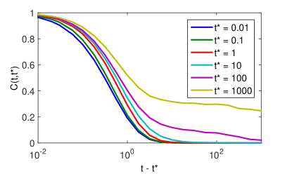
Figure 2: Aging curves: autocorrelation $C(t,t^{\ast})$ for $P\left(\mu\right)=\frac{2}{\sqrt{\pi}\mu^{2}}e^{-\mu^{-2}}$ in a system of size $M=1670$, averaged over 50 runs, showing that evolution becomes progressively slower but never stops. The times correspond to phases I to III.

Stage (I), continuous distributions

This stage lasts forever if the population $M$ is infinite. During these times, the population of every type is negligible with respect to $M$ i.e. $n_{a}\ll M\;\forall a$, so one may assume it to be a continuous function of $\lambda,\mu$ and time $t$. Let $\rho\left(\lambda,\mu,t\right)$ be the normalized distribution of individuals in a population. It satisfies

$$\dot{\rho}=-(L+\langle\lambda\rangle)\rho+\langle\mu\rangle\;p(\lambda,\mu)$$ (4)

where $\langle A\rangle\equiv\int d\mu d\lambda\;A\;\rho(\lambda,\mu,t)$ and $L$ is the genetic load, Eq. (3).

First, we consider the stationary distribution $\rho_{s}(\lambda,\mu)$, satisfying

$$(-\mu+\lambda-\langle\lambda\rangle_{s})\rho_{s}+\langle\mu\rangle_{s}\;p(\lambda,\mu)=0$$ (5)

(here $\langle A\rangle_{s}$ denotes average over $\rho_{s}$). If all the $\lambda$ are equal there is no selection pressure, and the evolution (4) converges in finite time to a stationary distribution

$$\rho_{stat}(\lambda,\mu)=\frac{p(\lambda,\mu)/\mu}{\int d\lambda d\mu\;p(\lambda,\mu)/\mu}$$ (6)

which is simply the distribution weighted with the residence time and always exists if the integral in the denominator is finite, which we assume throughout. The individuals spend time in attractors with finite lifetimes, making only rare visits to the more stable ones.

Something dramatic happens as soon as we switch on a many-valued fitness: the effect of any fitness distribution is to switch the system from short-lived to long-lived attractors. If $\mu_{min}=0$ the stationary solution disappears altogether (Eq. (5) has no solution, see Appendix A). This is a first order phase transition to a situation where the system forever evolves – ages – and population time-scales grow indefinitely, see Fig. 2. The individuals’ stability also increases, spending time in states with larger and larger time-scale $\tau=1/\mu$. For example, the increase of the lifetime is given by:

$$\langle\tau\rangle_{t}\geq\langle\mu\rangle_{t}^{-1}\sim t^{\gamma}$$ (7)

where we have used Jensen’s inequality, and the average is over the distribution at time $t$, see Fig. 3,(a). The exponent $\gamma$ is one when $P(\mu)$ is a power law, and $\gamma=1/\left(n+1\right)$ for $P\sim e^{-\mu^{-n}}$ (see Appendix C). In this regime, there is a clear selection pressure towards greater stability.

In order to quantify the correlations between stability and fitness, we calculate the correlation coefficient $C_{\lambda_{max}-\lambda,\mu}\left(t\right)$ between $\mu$ and $\lambda_{max}-\lambda$. The asymptotic value is always positive (see analytic expression Appendix D, Eq. (43)). See Fig. 3,(b) for Comparison between finite $M$ simulations, rate equations (Eq. (4)), and analytical asymptotics. Interestingly, models with strong memory (e.g. when fitness jumps are small) can develop an opposite, negative correlation between mutation and selection Gerrish .

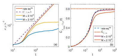
Figure 3: (a) Growth of individuals’ stability $\left\langle\mu\right\rangle^{-1}$ as a function of time, (b) Evolution of correlation $C_{\lambda_{max}-\lambda,\mu}\left(t\right)$, between stability and fitness. $C_{t\rightarrow\infty}$ is the analytic asymptotic result. Data for $P\left(\mu\right)=3\mu^{2}$, $\mu\leq 1$.

Stage (II), condensation

Finite population size $M$ effects cannot be neglected, because they can begin to show up at times of order $\ln M$, which for example in chemostat conditions may be a few tens of generations braun . Two effects compete here: on the one hand for finite $M$ there is an upper cutoff value $L{}_{c}=\mu_{c}-\lambda_{c}$, set by the probability of populating the tail with a single individual $\int_{\mu_{c}}^{\infty}\int_{\lambda_{c}}^{\lambda_{max}}d\mu d\lambda\rho(\lambda,\mu)\sim 1/M$. Secondly, there is the increase of the occupation of a few states $n_{a}$, an effect already found in simpler models Kingman ; Krug ; Krug1 ; silvio , analogous to the evolution of family names family_names . Here, this effect depends on $\mu$, and becomes especially strong for the small $\mu$.

The net result is that after a time that is logarithmic in $M$ for $P(\mu)\sim e^{-\mu^{-n}}$ and power law for power law tails at small $P(\mu)$, the distribution begins to have clusters at population in states of small $\mu$ (Fig. 1). At this point the continuous description in terms of a $\rho(\lambda,\mu,t)$ breaks down. At the end of this crossover, a large fraction of the population is in a single state having a $\mu_{d}$ of order $\ln M$ (or power law in $M$, for power law $P(\mu)$), while the rest of the population is distributed in many states, most of which are less stable and less fit.

Stage (III), Sweeps (Successional Mutation Regime)

From the condensation time up to times exponential in $M$, the system continues evolving by making rare and relatively rapid changes of the dominant state (‘sweeps’). Here a large number $M_{eff}^{a}$ individuals are in state $\left(\lambda_{a},\tau_{a}\right)$, but there is a ‘cloud’ of $M-M^{a}$ individuals which have suffered a deleterious mutation to a state with substantially smaller $\lambda$, constantly being renovated (see Figure 1). If the cloud has $\lambda_{cloud}\ll\lambda_{a}$, one can easily see that the dominant population size is

$$M_{eff}^{a}=M\left(1-\frac{\mu_{a}}{\lambda_{a}}\right)\,.$$ (8)

A sweep from a state $a$ to a state $b$ consists of a mutation in a single individual from $a$ to $b$, followed by growth of the $b$ sub-population until fixation, where $a$-state individuals have gone extinct. Mutations to lower $L=\mu-\lambda$ have a large probability of fixation,$O\left(M^{0}\right)$. Mutations to higher $L$ rarely fixate in the population, with probability exponentially small in $M$.

In a simple case when the cloud size is negligible (i.e. $\mu_{a}/\lambda_{a}\ll 1$ so $M_{eff}\simeq M$), the jump probability to $b$ in time $\delta t$ is well-known Nowak , $\delta p_{a\rightarrow b}=\delta t\,\mu_{a}\left(1-r_{ab}\right)/\left(1-r_{ab}^{M}\right)$, where $r_{ab}\equiv\lambda_{a}/\lambda_{b}$. For $\lambda_{b}>\lambda_{a}$ this is of order one even for large $M$, while for $\lambda_{b}<\lambda_{a}$ this is exponentially small in $M$, $\delta p_{a\rightarrow b}\sim\delta t\,\mu_{a}exp\left(-M\ln r_{ab}\right)$.

More generally, when a cloud is present and both $\lambda,\mu$ change their value, it is still true that $p_{a\rightarrow b}=O\left(M^{0}\right)$ when $L_{b}<L_{a}$. For $L_{a}<L_{b}$

$$p_{a\rightarrow b}\sim\delta t\,\mu_{a}exp\left(-\frac{M_{eff}^{2}}{M}\ln r_{ab}\right)\,,$$ (9)

where now $r_{ab}\equiv L_{a}/L_{b}$, and $L_{a}=\mu_{a}-\lambda_{a}$ is the genetic load as before. This holds for small changes in both $\lambda$ and $\mu$: $\left|\lambda_{b}/\lambda_{a}-1\right|,\left|\mu_{b}/\mu_{a}-1\right|\ll 1$. Here $M_{eff}\equiv M_{eff}^{a}\simeq M_{eff}^{b}$ (since changes in $\lambda$,$\mu$ are small). The calculation is described in Appendix E. Thus as in earlier stages, the genetic load $L_{a}=\mu_{a}-\lambda_{a}$ decreases as in a sequence of ‘record breaking’ events record_stats , except for random extinction events extinction which are exponentially suppressed in $M$.

In fact, as was noted before Berg_Lassig ; Berg_Willmann_Lassig ; Sella_Hirsh ; Brotto , Eq. (9) implies the relation

$$\frac{\delta p_{a\rightarrow b}}{\delta p_{b\rightarrow a}}\sim e^{\frac{M_{eff}^{2}}{M}(\ln L_{b}-\ln L_{a})}\,,$$ (10)

which may be interpreted as detailed balance relation, with temperature $T=M/M_{eff}^{2}$ and energy:

$$E_{a}=-\ln L_{a}$$ (11)

The evolution may hence be seen, once the system is in the successional mutation regime, as a relaxation within an energy landscape, Eq. (11), in contact with a bath of inverse temperature $M_{eff}^{2}/M$. If the jumps in $\lambda$ and $\mu$ are not small, detailed-balance does not generally hold.

In the above it was assumed that $Q(\lambda)$ has a bounded support $\lambda<\lambda_{max}$, in which case the dynamics does is to rather rapidly choose values of $\lambda_{a}\sim\lambda_{max}$, and decreasing $\mu_{a}$. If, on the other hand, $Q(\lambda)$ is not bounded, the situation is more subtle. One may still analyze the problem as an annealing of $E(\lambda,\mu)$, with an ‘entropy’ $S=\ln Q(\lambda)+\ln P(\mu)$. In any case, if the tail of $Q(\lambda)$ falls fast enough, it is always more convenient for the system to look for smaller $\mu$.

Stage (IV), saturation (‘Interrupted Aging’)

Finally, at (often unobservable) large times, the maximal possible improve in genetic load $\mu_{a}-\lambda_{a}-\mu_{max}+\lambda_{max}$ is such that the probability of a change decreasing genetic load becomes comparable to that of an ‘extinction process’ increasing it. At such time aging stops, the system has reached its stationary regime. In glassy physics this is known as ‘interrupted aging’ Bouchaud . From the point of view of a system in contact with a bath of temperature $T=M/M_{eff}^{2}$, the system has achieved thermal equilibrium

$$p(a)\propto e^{-\frac{M_{eff}^{2}}{M}E_{a}}\propto e^{-\frac{M_{eff}^{2}}{M}\ln L_{a}}$$ (12)

From this equation it is clear that for large $M$, small values of $\mu$ are selected, via the attempt to reduce $L$.

Positive $\mu_{min}$: crossover to ‘condensation’ dynamics.

When $\mu_{min}>0$ is strictly positive but small, the aging process we have described continues until $\langle\mu\rangle(t)$ decreases to order of $\mu_{min}$. This may take very long, especially if the distribution $P(\mu)$ falls fast, at which case the lower bound on $\mu$ becomes irrelevant.

Let us consider first the case when $M$ is infinite. There is a critical value $\lambda_{max}^{c}$: a) If $\lambda_{max}<\lambda_{max}^{c}$, Eq. (5) has a smooth solution, the system has a stationary distribution with many attractors having finite timescales, and starting from any state, stationarity is reached in finite times. b) If $\lambda_{max}>\lambda_{c}$ the system has a stationary distribution $\rho(\lambda,\mu)=\tilde{\rho}(\lambda,\mu)+a\delta(\mu-\mu_{min})\delta(\lambda-\lambda_{max})$ with a continuous part $\tilde{\rho}(\lambda,\mu)$ plus a finite fraction $a$ of the population concentrated in $(\lambda_{max},\mu_{min})$, see Appendix B for details. This phenomenon is closely analogous to Bose-Einstein condensation in solid state physics, and has been encountered previously in other evolving systems silvio . In an experiment starting from a random configuration, the system will evolve towards this distribution, but condensation of a finite fraction in $(\lambda_{max},\mu_{min})$ necessarily takes times divergent with $M$. As before, the population ages, occupying states with $\left(\lambda,\mu\right)$-values which are increasingly closer to $(\lambda_{max},\mu_{min})$. An example of a phase-diagram is given in Appendix B. This transition is analogous to Eigen’s mutational meltdown eigen , where evolution is hampered by high mutation rates.

If on the other hand both $M$ and $\mu_{min}$ are finite, the system has a complex behavior of competition between the condensation effect due to finiteness of $\mu_{min}$ at infinite $M$ and those due to finiteness of $M$ (i.e. equilibration, stages (II) and (III)).

Relation between fitness and mutation rate in the well-mixed case

Let us now summarize how the individuals’ stability $\tau=1/\mu$ is selected in the different stages.

In the continuous Stage I the average of $\tau$ grows steadily as $\langle\tau\rangle\geq\langle\mu\rangle^{-1}\sim t^{\gamma}$ where $\gamma$ depends on the distributions.

Once in Stage III, the dominant type changes in rather fast sweeps. Mutations to lower $L=\mu-\lambda$ have a significant probability of fixation, while fixations to higher $L$ are rare. Therefore mutation rates decrease as growth rates increase. If $P(\lambda)$ has a bounded support $\lambda<\lambda_{max}$, what the dynamics does is to rather rapidly choose values of $\lambda_{i}\sim\lambda_{max}$, and increasing $\tau_{i}$. If, on the other hand, $P(\lambda)$ is not bounded, the situation is more subtle. One may analyze the problem as an annealing of $E(\lambda,\mu)$, see Eq. (11) with an ‘entropy’ $S=\ln Q(\lambda)+\ln P(\mu)$. In any case, if the tail of $Q(\lambda)$ falls fast enough, it is always more convenient for the system to look for smaller $\mu$.

Finally, phase (IV), corresponding to equilibrium, may be analyzed directly on the basis of Eq (12). It is clear that in this final value large values of $\mu$ are selected.

II Expansion in space

Let us turn to a situation where the limited resource is not nutrient, but rather space. We model spatial expansion in two and three dimensions with cells growing radially or confined between walls as follows: cells are modeled as circles (or spheres in three-dimensions) of equal radius. They attempt to reproduce with a rate $\lambda$. The offspring (having the same $\lambda$ and $\mu$), is created in contact with the parent cell - if there is no free place in contact with the mother cell reproduction does not happen. Just as in the previous section, cells mutate to with their rate $\mu$ to a new state with $(\lambda^{\prime},\mu^{\prime})$ chosen with probability $Q(\lambda^{\prime})P(\mu^{\prime})$. Cells in the bulk of the colony produce no more progeny, but they keep on mutating.

Here we are interested in the following question: what is the effect of a dispersion in the values of mutation rate $\mu$? Unlike the case of a well-mixed system, where the ‘genetic load’ (the rate loss of population of a state) was naturally $L_{a}=\mu_{a}-\lambda_{a}$, and this led naturally to a decrease in $\mu$ in the population, here it is not clear if this should happen at all. As it turns out, even in this spatial version smaller $\mu$ are selected, but the way this happens is less obvious.

In order to understand the basic mechanism, following Refs. KuhrFrey ; Lavrentovich , we first consider cells that may be in only two states, with $\lambda_{f}>\lambda_{s}$. We consider the growth of a linear front between two walls (Fig. 4). The dominating ‘fast’ type mutates into the ‘slow’ type with typical time-scale $1/\mu$, which we assume is large so that a large colony is essentially composed of ‘fit’ cells with $\lambda_{f}$, with occasional ‘spots’ of cells that where born ‘unfit’, with $\lambda_{s}$. (A complete extinction of the cells with $\lambda_{f}$ would be irreversible, but its probability vanishes with the size if $\lambda_{f}>\lambda_{s}$).

The results for the colony length $G$ are shown in Fig. 5: the growth rate of a $\lambda_{f}$-rich population is indeed slowed down by the mutations. The reason is simple: a mutation creates a ‘spot’ of slowly reproducing cells with $\lambda_{s}$, which becomes an obstacle and delays the advance of the from of cells with $\lambda_{f}$. If $\lambda_{s}=0$, the mutated cells leave no offspring, but for larger values of $\lambda_{s}$ the ‘bad spots’ become larger – although less inefficient. In order to quantify the interplay between fitness and stability, consider the case when $\tau$ is so large that two different spots due to different mutations do not overlap. The retardation factor $R$ on the growth length $G$, with respect to $G_{\infty}$ – the one that would be obtained without deleterious mutations – is then proportional to the density of spots, in turn $\propto\mu$, and we get:

$$R\equiv\frac{G_{\infty}-G}{G_{\infty}}=A(\lambda_{s}/\lambda_{f})\;\frac{\mu}{\lambda_{f}}$$ (13)

The function $A(\lambda_{s}/\lambda_{f})$ is the retardation per unit ‘spot’, which depends on the dimension and on the details of the dynamics. We have computed $G$ numerically in two and three dimensions, and we find that (see Fig. 5) $A(\lambda_{s}/\lambda_{f})$ is a growing function of $\lambda_{s}/\lambda_{f}$: The net counter intuitive result is that ‘bad’ mutations are more deleterious if they are just barely worse, $\lambda_{s}\lesssim\lambda_{f}$, while they are more innocent if they are completely sterile ($\lambda_{s}=0$).

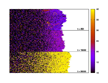
Figure 4: Population of cells growing between two walls (along x direction, left to right) with a distribution of $(\lambda,\mu)$ given by $Q(\lambda)P(\mu)$. The figure shows three snapshots of the more advanced $\Delta G$ of the growing colony, at times $t=250,15000,30000$. The color code refers to the values of $1/\mu$ of particles. The front layer of the colony is composed of cells selected to have unusually low mutation rate, and consistently, this layer becomes thicker with time.

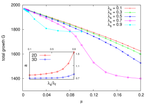
Figure 5: Values of the total linear growth $G$ for a clone with two states $\lambda_{f}$ and $\lambda_{s}$. The plots are for $\lambda_{f}=1$ and different values of mutation rates $\mu$ and $\lambda_{s}$. The is linear regime for small $\mu$ (independent ‘spots’) with gradient $-A(\lambda_{s})$, which is the one described by equation (13). Surprisingly enough, growth is more strongly retarded for higher values of $\lambda_{s}$, meaning that deleterious mutations are worse when they are not completely sterile. (In the curves for $\lambda_{s}=0.7$ and $0.9$, one can see the transition to the inactive phase, signaled in the steep drop in the values of the colony growth for high $\mu$ values.)

Consider next two spatially adjacent colonies with only two states as above, $(\lambda_{f}^{1},\lambda_{s}^{1},\mu^{1})$, $(\lambda_{f}^{2},\lambda_{s}^{2},\mu^{2})$, respectively. The case of two competing colonies with ($\lambda_{1}$,$\lambda_{2}$) and no mutations allowed ($\mu_{1}=\mu_{2}=0$), has been studied extensively by Korolev et al. HallaNelson . The colony with the highest $\lambda$ prevails, the time for the overcome scales linearly in $\Delta\lambda$ in the case of colony growing with a linear front, while it scales logarithmically in a radial, two-dimensional growth. Here, the relevant parameters for the competition of the colonies are not $\lambda_{f}^{1}$ and $\lambda_{f}^{2}$, but rather their net growth rate $\lambda_{f}^{1}(1-R_{1})$ and $\lambda_{f}^{2}(1-R_{2})$, which is affected by their respective ‘retardation’ factors of $R_{1}$ and $R_{2}$ calculated as in Eq. (13).

Fig. 6 shows two competing sets with the same fitness $\lambda_{f}^{1}=\lambda_{f}^{2}$, $\lambda_{s}^{1}=\lambda_{s}^{2}$, but different values of $\mu$, and hence different $R$’s. The type with the smallest $\tau$ becomes extinct, because of the slowing down provoked by the occasional mutations, which are more frequent in one case than in the other.

In a spatial setting it is important to notice that the relevant dynamics and the effects of selection are present only at the advancing front of the colony. In the bulk, where cells have no more space to reproduce, if we assume they may continue to mutate they eventually go to equilibrium, i.e. the bulk population eventually (in a finite time) will sample the original probability distribution for $\lambda$ and $\mu$, therefore losing any evolutionary achievement the system had reached.

We are now in a position to return to the original model, with a distribution of values of $\lambda$ and $\mu$. The sequence of phases described in the well-mixed case is present, with the same features, also in the spatial setting with competing colonies, as already discussed by Desai and Fisher Fisher1 . At late stages, when the evolution is essentially successional, the situation is quite similar to the one discussed in the simplified models above. There is a dominant type with $\lambda_{f}$ close to the optimum, and there will be occasional mutations, most of which will produce less fit cells. This yield unsuccessful ‘spots’ of low fitness, that retard the advance, just as in the simpler example above. The only difference with the ‘two-type’ version is that the value of $\lambda_{s}$ will not be fixed, but taken from the $Q(\lambda)$ distribution, which has the only effect of modifying the function $A$ in Eq. (13) to a $Q$-dependent function $A_{Q}$. When a mutation finally produces a lineage with smaller $L=A_{Q}\mu-\lambda$, it will with high probability overcome the dominant one, even if it has a lower $\lambda_{f}$.

All in all we find the non-trivial geometric factor $A_{Q}$ which modifies the genetic load with respect to the well-mixed case, but otherwise produces the same selection of large $\mu$’s effect. $A_{Q}$ turns out to be greater in two spatial dimensions than in 3D, and it is of order one. In Fig. 4 we see how selection comes about in a population as the one described for the well-mixed case: the cells at the front are the most stable ones.

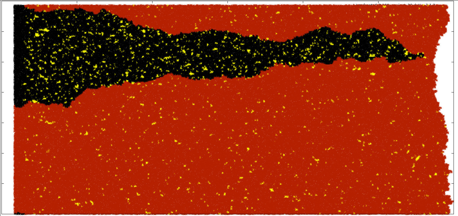
Figure 6: Competition between two species of cells with equal $\lambda_{f}$, mutating into equal $\lambda_{s}=0.3\lambda_{f}$, but with two different mutation rates. The first species (black) has $\mu_{1}=1/20$, while the second one (red) has $\mu_{2}=1/100$. Particles which mutated while in the front are shown in yellow. At the beginning (far left) the two species have the same number of cells. The second species grows faster and overtakes the first one. This can be seen also by looking at the front shape after the overcoming: the front to the right of the black species is retarded. The effect is only due to a difference in the mutation rate $\tau$: the colony composed of stabler cells prevails.

III Conclusions

The stability and reproduction rates become correlated for a population even if there was no such mechanism for the single individual to start with. If one considers the statistics at long times, a large part of the population is in very fit (high $\lambda$) and very stable (low $\mu$) states, while the rest of the population is in states that have intermediate values of both $\lambda$ and $\mu$: the fittest tend to be the stablest individuals. This conclusion seems to be valid whatever the mechanism that limits the population. If we observed an internal (e.g. chemical) mechanism that is responsible for the higher stability of some cells, we might conclude that it is a well-designed response of an individual cell tailored to lower its mutation rate under favorable conditions. It could be, however, that as in our case there is no such mechanism, and the correlation only arises at the level of population, for purely statistical reasons. In order to test whether an adaptive mechanism that changes mutation rate in response to external conditions exist – that is to say: whether fitness and mutation rates correlate for the states of a single cell – we could try following the changes of a single individual, ignoring its progeny. Another relation between fitness and mutation rate appears when the environment changes: changes in the fitness of states $\lambda_{a}$ amount to ‘rejuvenating’ (reinitializing) the system: this brings about a drop in both the fitness and the average mutation time (see Leibler ).

‘Population Aging’ in which the dynamics slows down arises also as a purely collective effect (see Ref. Krug ), with the added element that the stability of the individuals themselves also increases. The slowing down of the dynamics may be checked by means of an experiment to test the divergence time $t_{div}$ of subpopulations isolated at different $t^{*}$.

Acknowledgments

We wish to thank A. Amir, E. Braun, N. Brenner and L. Peliti for useful suggestions. G.B. acknowledges the support of the Chateaubriand Fellowship and the Pappalardo Fellowship in Physics. T.B. acknowledges the support of UIF/UFI (Bando Vinci).

Appendices

Appendix A: The stationary solution, and the $\mu_{min}=0$ case

Denote $R_{\mu}\equiv\left\langle\mu\right\rangle\equiv\int d\mu d\lambda\mu\rho\left(\lambda,\mu\right)$, and $R_{\lambda}\equiv\left\langle\lambda\right\rangle=\int d\mu d\lambda\rho\left(\lambda,\mu\right)\lambda$.

$p(\lambda,\mu)$ is defined on $\lambda_{\min}<\lambda<\lambda_{max}=1$ and $0\leq\mu_{min}<\mu<\mu_{max}$. The condition for stationarity is

$$\dot{\rho}_{s}=\left[\lambda-\mu-R_{\lambda}\right]\rho_{s}+R_{\mu}p(\lambda,\mu)=0\ ,$$ (14)

which gives the stationary $\rho_{s}\left(\lambda,\mu\right)$

$$\rho_{s}(\lambda,\mu)=\frac{R_{\mu}p(\lambda,\mu)}{\mu-\lambda+R_{\lambda}}\ .$$ (15)

We look for the conditions under which $\rho_{s}\left(\lambda,\mu\right)$ exists, and is a smooth function that is not everywhere zero. The last condition requires $R_{\mu}>0$.

If $R_{\mu}=0$, no normalizable steady-state solution exists. As we show in the next section, the system will age.

Assuming these conditions are met, we obtain

$$1 =R_{\mu}\int d\lambda d\mu\;\frac{p(\lambda,\mu)}{\mu-\lambda+R_{\lambda}}\ ,$$ (16)

$$R_{\mu} =R_{\mu}\int d\lambda d\mu\;\frac{\mu\;p(\lambda,\mu)}{\mu-\lambda+R_{\lambda}}\ ,$$ (17)

$$R_{\lambda} =R_{\mu}\int d\lambda d\mu\;\frac{\lambda\;p(\lambda,\mu)}{\mu-\lambda+R_{\lambda}}\ .$$ (18)

Of the three equations only two are independent.

From Eq. (17), if $R_{\mu}>0$ then

$$1=\int d\lambda d\mu\frac{\mu\;p(\lambda,\mu)}{\mu-\lambda+R_{\lambda}}\ ,$$ (19)

which fixes $R_{\lambda}$. In that case, $R_{\mu}$ is obtained from the Eq. (18).

We note the following:

$\bullet$ For $R_{\mu}>0$, the integral in Eq. (16) must be finite, so the integral must converge which requires $R_{\lambda}\geq\lambda_{max}-\mu_{min}$. We also have $R_{\lambda}=\left\langle\lambda\right\rangle\leq\lambda_{max}$. Therefore, if $\mu_{min}=0$, we find $R_{\lambda}=\lambda_{max}$. But then Eq. (19) cannot be satisfied for general $p(\lambda,\mu)$. We conclude that if $\mu_{min}=0$ then $R_{\mu}=0$ and $R_{\lambda}=\lambda_{max}$.

$\bullet$ If $\mu_{min}>0$ there may be a solution to equation (19) with $R_{\lambda}\neq\lambda_{max}$. Note that if $\lambda_{\min}=\lambda_{\max}$ Eq. (19) is automatically satisfied, so there is always a smooth solution. Hence, for $\mu_{min}=0$ the system ages as soon as there is any dispersion in the possible values of $\lambda$.

Appendix B: $\mu_{min}>0$ condensation

If $\mu_{min}>0$ and there is no smooth solution, we must extend the solution space. We attempt the following $\rho=\rho_{smooth}+a\delta(\lambda-\lambda_{max})\delta(\mu-\mu_{min})$, meaning that a condensate forms at a single trap at $\left(\lambda_{max},\mu_{min}\right)$. Let $D_{\varepsilon}$ be a small region in $\left(\lambda,\mu\right)$-space that contains the point $\left(\lambda_{max},\mu_{min}\right)$. Integrating the stationary condition, Eq. (14), over $D_{\varepsilon}$ we find

$$a\cdot\left(\lambda_{max}-\mu_{min}-R_{\lambda}\right)+\int_{D_{\varepsilon}}d\lambda d\mu\left[\left(\lambda-\mu-R_{\lambda}\right)\rho_{smooth}+R_{\mu}p(\lambda,\mu)\right]=0\ ,$$

and as the area of $D_{\varepsilon}$ goes to zero, this approaches $a\cdot\left(\lambda_{max}-\mu_{min}-R_{\lambda}\right)=0$, so that $R_{\lambda}=\lambda_{max}-\mu_{min}$ for $a\neq 0$. The two independent equations (16,17) now read

$$1 =a+R_{\mu}\int d\lambda d\mu\frac{p(\lambda,\mu)}{\mu-\lambda+R_{\lambda}}\ ,$$

$$R_{\mu} =a\mu_{min}+R_{\mu}\int d\lambda d\mu\frac{\mu\ p(\lambda,\mu)}{\mu-\lambda+R_{\lambda}}\ ,$$ (20)

and obtain

$$a=\frac{1-\int d\lambda d\mu\frac{\mu\ p(\lambda,\mu)}{\mu-\lambda+R_{\lambda}}}{1-\int d\lambda d\mu\frac{p(\lambda,\mu)}{R_{\lambda}-\lambda+\mu}\left(\mu-\mu_{min}\right)}\ ,$$ (21)

which using $R_{\lambda}=\lambda_{max}-\mu_{min}$ fixes $a$. In Fig. 7, an example of a phase diagram is shown, for $p\left(\mu\right)\propto\mu^{-2}e^{-1/\mu}$. Below the line, a solution with $a>0$ exists; Above the line, a solution to Eq. (14) exists.

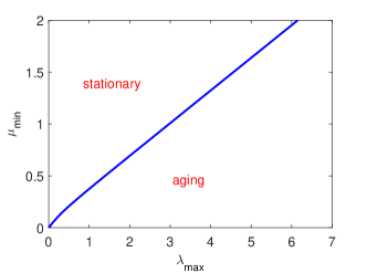
Figure 7: The phase diagram in terms of $\lambda_{max}$ and $\mu_{min}$, for $p\left(\mu\right)\propto\mu^{-2}e^{-1/\mu}$ in $\left[\mu_{min},\infty\right]$. Similar diagrams arise in glassy models with metastable states garrahan .

Appendix C: Aging for the $M=\infty$ case

In the following, to make expressions simpler we take $\lambda_{max}=1$, which can always be obtained by rescaling time. Denote $u\equiv 1-\lambda$. The time-dependent solution for $\rho$ is

$$\rho=p\left(\lambda,\mu\right)\int_{0}^{t}dt^{\prime}e^{-\left(u+\mu\right)\left(t-t^{\prime}\right)}e^{\int_{t^{\prime}}^{t}R_{1-\lambda}\left(t^{\prime}\right)dt^{\prime}}R_{\mu}\left(t^{\prime}\right)+\rho_{0}e^{-\left[\left(u+\mu\right)t+\int_{0}^{t}R_{1-\lambda}\left(t^{\prime}\right)dt^{\prime}\right]}\ .$$

The time-dependent equivalents of Eq. (16,17,18) read

$$1 =e^{\int_{0}^{t}R_{1-\lambda}(t^{\prime\prime})dt"}\int_{0}^{t}dt^{\prime}f(t^{\prime})\;I(t-t^{\prime})+const\cdot e^{-\int_{0}^{t}R_{1-\lambda}(t^{\prime\prime})dt"}$$

$$R_{\mu} =e^{\int_{0}^{t}R_{1-\lambda}(t^{\prime\prime})dt"}\int_{0}^{t}dt^{\prime}f(t^{\prime})\;I_{\mu}(t-t^{\prime})+\;const^{\prime}e^{-\int_{0}^{t}R_{1-\lambda}(t^{\prime\prime})dt"}$$

$$R_{1-\lambda} =e^{\int_{0}^{t}R_{1-\lambda}(t^{\prime\prime})dt"}\int_{0}^{t}dt^{\prime}f(t^{\prime})\;I_{1-\lambda}(t-t^{\prime})+const^{\prime\prime}e^{-\int_{0}^{t}R_{1-\lambda}(t^{\prime\prime})dt"}$$ (22)

the functions $I\left(t\right),I_{\mu}\left(t\right),I_{1-\lambda}\left(t\right)$ are defined as

$$I\left(t\right) \equiv\int d\mu d\lambda p\left(\lambda,\mu\right)e^{-\left(u+\mu\right)t}$$

$$I_{\mu}\left(t\right) \equiv\int d\mu d\lambda\mu p\left(\lambda,\mu\right)e^{-\left(u+\mu\right)t}$$

$$I_{1-\lambda}\left(t\right) \equiv\int d\mu d\lambda\left(1-\lambda\right)p\left(\lambda,\mu\right)e^{-\left(u+\mu\right)t}$$ (23)

and

$$f(t)\equiv R_{\mu}(t)e^{-\int_{0}^{t}R_{1-\lambda}(t^{\prime\prime})dt"}\ .$$ (24)

We are now interested in the large time behavior of $R_{\mu}$ and $R_{1-\lambda}\equiv\left\langle 1-\lambda\right\rangle$. (As before, we take $\lambda_{max}=1$.) If the initial condition has support only over $\mu>0$, the result does not depend on the last term in the three equations for large times. We shall use the following result: if both $f$ and $I_{\ast}$ decrease as a power-law or exponent, then for large times

$$\int_{0}^{t}\;f(t^{\prime})I_{\ast}(t-t^{\prime})dt^{\prime}\sim f(t)\;\left[\int_{0}^{\infty}dt^{\prime}\;I_{\ast}(t^{\prime})\right]+I_{\ast}(t)\;\left[\int_{0}^{\infty}dt^{\prime}\;f(t^{\prime})\right]$$ (25)

Unless both fall equally fast, only one of these two terms contribute. We shall assume (and later check) that $I(t)$ falls slower than $f(t)$. Then, the first of Eq. (22) becomes

$$1=e^{\int_{0}^{t}R_{1-\lambda}(t^{\prime\prime})dt"}\;I(t)\;\left[\int_{0}^{\infty}dt^{\prime}\;f(t^{\prime})\right]$$ (26)

which means that

$$R_{1-\lambda}(t)\sim-\frac{\partial\ln I(t)}{\partial t}$$ (27)

Next, we shall assume that $I_{\mu}$ fall as fast as $f(t)$. We have that the second of Eq. (22) reads:

$$R_{\mu}=e^{\int_{0}^{t}R_{1-\lambda}(t^{\prime\prime})dt"}\left\{f(t)\;\left[\int_{0}^{\infty}dt^{\prime}\;I_{\mu}(t^{\prime})\right]+I_{\mu}(t)\;\left[\int_{0}^{\infty}dt^{\prime}\;f(t^{\prime})\right]\right\}$$ (28)

Dividing by the expression for $f$ we find

$$R_{\mu}\propto\left\{\frac{f(t)}{I(t)}\;\left[\int_{0}^{\infty}dt^{\prime}\;I_{\mu}(t^{\prime})\right]+\frac{I_{\mu}(t)}{I(t)}\;\left[\int_{0}^{\infty}dt^{\prime}\;f(t^{\prime})\right]\right\}$$ (29)

which by assumption grows as $\frac{I_{\mu}(t)}{I(t)}$ does. Finally, $I_{1-\lambda}$ falls faster than both $f$ and $I_{\mu}$ so that:

$$R_{1-\lambda}=e^{\int_{0}^{t}R_{1-\lambda}(t^{\prime\prime})dt"}f(t)\;\left[\int_{0}^{\infty}dt^{\prime}\;I_{1-\lambda}(t)\right]\propto R_{\mu}(t)$$ (30)

where we have used the previous expression for $f$.

Let us now give some examples. Performing the integral over $\lambda$, we get:

$$I(t) =\frac{1-e^{-t}}{t}\int d\mu\;p(\mu)e^{-\mu t}$$

$$I_{\mu}(t) =\frac{1-e^{-t}}{t}\int d\mu\;\mu p(\mu)e^{-\mu t}$$

$$I_{1-\lambda}(t) =\frac{1-e^{-t}(1-t)}{t^{2}}\int d\mu\;p(\mu)e^{-\mu t}$$ (31)

$\bullet$ Power law $P(\mu)$. If $P(\mu)\propto\mu^{\alpha}$, and $Q\left(\lambda\right)=1$ on $\lambda\in\left[0,1\right]$: We have that $\int d\mu\;p(\mu)e^{-\mu t}\sim t^{-\alpha+1}$ and $\int d\mu\;\mu p(\mu)e^{-\mu t}\sim t^{-\alpha}$, so that for large $t$ we get:

$$I(t) \sim t^{-\alpha}$$

$$I_{\mu}(t) \sim t^{-\alpha-1}$$

$$I_{1-\lambda}(t) \sim\frac{1}{t}I(t)$$ (32)

Equations (27) and (30) give:

$$R_{1-\lambda}(t) \sim-\frac{\alpha}{t}$$ (33)

$$R_{\mu}(t) \propto t^{-1}$$ (34)

$\bullet$ Strongly suppressed $P(\mu)$. If $P(\mu)\propto e^{-b\mu^{-n}}$, and $Q\left(\lambda\right)=1$ on $\lambda\in\left[0,1\right]$: The integrals over $P(\mu)$ may be evaluated by saddle point. The saddle point is $\mu_{sp}=\left(\frac{t}{bn}\right)^{-\frac{1}{n+1}}$. We get

$$I(t)=e^{\left(\frac{t}{t_{0}}\right)^{-\frac{n}{n+1}}}\;\;\;;\;\;\;\frac{I_{\mu}}{I}=\mu_{sp}=\left(\frac{t}{bn}\right)^{-\frac{1}{n+1}}$$ (35)

and:

$$R_{1-\lambda}(t) \sim t^{-\frac{1}{n+1}}$$ (36)

$$R_{\mu}(t) \propto t^{-\frac{1}{n+1}}$$ (37)

$\bullet$ Other $Q\left(\lambda\right)$. The above results are unchanged if more generally, $P\left(\lambda\right)=\left(1-\lambda\right)^{m}$ with $m>0$, for $\lambda$ around $1$. The power of $I(t)$ changes, but $R_{1-\lambda}(t)\sim-\frac{\partial\ln I(t)}{\partial t}$ is unchanged, and $R_{1-\lambda}\sim R_{\mu}(t)$.

In all cases one may check that these asymptotics are consistent with the initial assumptions.

Appendix D: Correlations between fitness and stability

To study correlations we introduce

$$R_{\mu,1-\lambda}\equiv\left\langle\left(1-\lambda\right)\mu\right\rangle=e^{\int_{0}^{t}R_{1-\lambda}(t^{\prime\prime})dt"}\int_{0}^{t}dt^{\prime}f(t^{\prime})\;I_{\mu,1-\lambda}(t-t^{\prime})+\;const^{\prime}e^{-\int_{0}^{t}R_{1-\lambda}(t^{\prime\prime})dt"}$$ (38)

where

$$I_{\mu,1-\lambda}\left(t\right)\equiv\int d\mu d\lambda\mu\left(1-\lambda\right)p\left(\lambda,\mu\right)e^{-\left(u+\omega\right)t}\ .$$ (39)

For $P\left(\lambda\right)=const$:

$$I_{\mu,1-\lambda}\left(t\right) =\int d\mu\mu P\left(\mu\right)e^{-\mu t}\int d\lambda\left(1-\lambda\right)Q\left(\lambda\right)e^{-\left(1-\lambda\right)t}=-\frac{e^{-t}(1-t)-1}{t^{2}}\int d\mu P(\mu)\mu e^{-\mu t}$$

$$=\frac{1-e^{-t}(1-t)}{1-e^{-t}}\frac{1}{t}I_{\mu}(t)\sim\frac{1}{t}I_{\mu}(t)$$

$$I_{\mu^{2}}\left(t\right) =\frac{1-e^{-t}}{t}\int d\mu P(\mu)\mu^{2}e^{-\mu t}\simeq\frac{1}{t}\int d\mu P(\mu)\mu^{2}e^{-\mu t}$$

$$I_{\left(1-\lambda\right)^{2}}\left(t\right) =\frac{e^{-t}\left(2e^{t}-2t-t^{2}-2\right)}{t^{3}}\int d\mu P(\mu)e^{-\mu t}\simeq\frac{2}{t^{3}}\int d\mu P(\mu)e^{-\mu t}$$ (40)

As $f(t)\sim I_{\mu}$, we have that that $I_{\mu,1-\lambda}\left(t\right)$ falls faster than $f\left(t\right)$. This is also true for $I_{\mu^{2}}\left(t\right),I_{\left(1-\lambda\right)^{2}}\left(t\right)$. Therefore

$$R_{\mu,1-\lambda}\left(t\right)\sim e^{\int_{0}^{t}R_{1-\lambda}(t^{\prime\prime})dt"}f(t)\;\left[\int_{0}^{\infty}dt^{\prime}\;I_{\mu,1-\lambda}\left(t^{\prime}\right)\right]=R_{\mu}(t)\;\left[\int_{0}^{\infty}dt^{\prime}\;I_{\mu,1-\lambda}\left(t^{\prime}\right)\right]\ ,$$ (41)

so $\left\langle\mu\left(1-\lambda\right)\right\rangle\sim R_{\mu}(t)\gg R_{\mu}(t)R_{1-\lambda}\left(t\right)\sim\left\langle\mu\right\rangle\left\langle 1-\lambda\right\rangle$, and at large times $\left\langle\mu\left(1-\lambda\right)\right\rangle/\left\langle\mu\right\rangle\left\langle 1-\lambda\right\rangle\sim 1/\left\langle\mu\right\rangle\sim\left\langle 1/\mu\right\rangle$, where the last equality holds at least in the 3 cases considered. To compute the correlation coefficient we use

$$R_{\mu^{2}}\left(t\right) =R_{\mu}(t)\;\left[\int_{0}^{\infty}dt^{\prime}\;I_{\mu^{2}}\left(t^{\prime}\right)\right]$$

$$R_{\left(1-\lambda\right)^{2}}\left(t\right) =R_{\mu}(t)\;\left[\int_{0}^{\infty}dt^{\prime}\;I_{\left(1-\lambda\right)^{2}}\left(t^{\prime}\right)\right]$$

$$\left\langle\mu^{2}\right\rangle-\left\langle\mu\right\rangle^{2} =R_{\mu}(t)\;\left[\int_{0}^{\infty}dt^{\prime}\;I_{\mu^{2}}\left(t^{\prime}\right)\right]-\left[R_{\mu}(t)\right]^{2}\left[\int_{0}^{\infty}dt^{\prime}\;I_{\mu}\left(t^{\prime}\right)\right]^{2}\sim R_{\mu^{2}}\left(t\right)$$

$$\left\langle\left(1-\lambda\right)^{2}\right\rangle-\left\langle 1-\lambda\right\rangle^{2} \sim R_{\left(1-\lambda\right)^{2}}\left(t\right)$$ (42)

so the correlation coefficient

$$C_{1-\lambda,\mu}\left(t\right) \equiv\frac{\left\langle\mu\left(1-\lambda\right)\right\rangle-\left\langle\mu\right\rangle\left\langle 1-\lambda\right\rangle}{\sqrt{\left[\left\langle\mu^{2}\right\rangle-\left\langle\mu\right\rangle^{2}\right]\left[\left\langle\left(1-\lambda\right)^{2}\right\rangle-\left\langle 1-\lambda\right\rangle^{2}\right]}}$$

$$\sim\frac{R_{\mu,1-\lambda}\left(t\right)}{\sqrt{R_{\mu^{2}}\left(t\right)R_{\left(1-\lambda\right)^{2}}\left(t\right)}}\underset{t\rightarrow\infty}{\longrightarrow}\frac{\int_{0}^{\infty}dt^{\prime}\;I_{\mu,\left(1-\lambda\right)}\left(t^{\prime}\right)}{\sqrt{\left[\int_{0}^{\infty}dt^{\prime}\;I_{\mu^{2}}\left(t^{\prime}\right)\right]\left[\int_{0}^{\infty}dt^{\prime}\;I_{\left(1-\lambda\right)^{2}}\left(t^{\prime}\right)\right]}}$$ (43)

As the integrands in the last expression are positive we have that $C_{1-\lambda,\mu}(t\rightarrow\infty)\geq 0$. Note that its exact value depends on the entire distributions of $P\left(\mu\right),Q\left(\lambda\right)$, while the long time behavior of $R_{\mu}(t)$, Eqs. (34,37), depends only on the tails of the distributions.

By keeping track of the corrections to the asymptotic value, one can show that $\left|C_{1-\lambda,\mu}\left(t\rightarrow\infty\right)-C_{1-\lambda,\mu}\left(t\right)\right|$ approaches zero with the same long time behavior derived in the Aging section above.

Appendix E: fixation probability in the presence of a cloud

In this Appendix the derivation of Eq. (9) is sketched. More precisely, it is shown that if $\lambda_{b}=\lambda_{a}\left(1+\varepsilon\right)$ and $\mu_{b}=\mu_{a}\left(1+\varepsilon_{\mu}\right)$ with $\left|\varepsilon_{\mu}\right|,\left|\varepsilon\right|\ll 1$, then for $\frac{L_{a}}{L_{b}}<1$ the probability that a single $b$-mutant will fix in the population is

$$\ln p_{a\rightarrow b}^{fix}=-\frac{M_{eff}^{2}}{M}\ln\frac{L_{a}}{L_{b}}$$

up to subleading corrections, of order $\ln M$. For notational simplicity we describe the case $\mu_{b}=\mu_{a}$$\equiv\mu$, and $\lambda_{b}=\lambda_{a}\left(1+\varepsilon\right)$, the more general case with $\varepsilon_{\mu}\neq 0$ follows from a similar argument. Note that the cloud size is not assumed to be negligible. The cloud individuals are assumed to have negligible self-reproduction, $\lambda_{c}=0$.

The stochastic process is described by $\left(n_{a},n_{b},n_{c}\right)$, the number of individuals in states $a,b$ and the cloud respectively, such that $n_{a}+n_{b},+n_{c}=M$. The reactions are

$$\left(n_{a},n_{b},n_{c}\right)\underset{\lambda_{a}\frac{1}{M}n_{a}n_{b}}{\longrightarrow}\left(n_{a}+1,n_{b}-1,n_{c}\right)\ \ \ ;\ \ \ \left(n_{a},n_{b},n_{c}\right)\underset{\lambda_{b}\frac{1}{M}n_{a}n_{b}}{\longrightarrow}\left(n_{a}-1,n_{b}+1,n_{c}\right)$$

$$\left(n_{a},n_{b},n_{c}\right)\underset{\lambda_{a}\frac{1}{M}n_{a}n_{c}}{\longrightarrow}\left(n_{a}+1,n_{b},n_{c}-1\right)\ \ \ ;\ \ \ \left(n_{a},n_{b},n_{c}\right)\underset{\lambda_{b}\frac{1}{M}n_{b}n_{c}}{\longrightarrow}\left(n_{a},n_{b}+1,n_{c}-1\right)$$

$$\left(n_{a},n_{b},n_{c}\right)\underset{\mu_{a}n_{a}}{\longrightarrow}\left(n_{a}-1,n_{b},n_{c}+1\right)\ \ \ ;\ \ \ \left(n_{a},n_{b},n_{c}\right)\underset{\mu_{b}n_{b}}{\longrightarrow}\left(n_{a},n_{b}-1,n_{c}+1\right)$$

Using standard large-deviation techniques [[refs]], we need to find the solution (‘instanton’) to Hamilton’s equations with the Hamiltonian

$$H =\left[\left(e^{\hat{n}_{a}-\hat{n}_{b}}-1\right)\frac{\lambda_{a}}{M}+\left(e^{\hat{n}_{b}-\hat{n}_{a}}-1\right)\frac{\lambda_{b}}{M}\right]n_{a}n_{b}$$

$$+\left(e^{\hat{n}_{a}-\hat{n}_{c}}-1\right)n_{a}n_{c}\frac{\lambda_{a}}{M}+\mu\left(e^{\hat{n}_{c}-\hat{n}_{a}}-1\right)n_{a}$$

$$+\left(e^{\hat{n}_{b}-\hat{n}_{c}}-1\right)n_{b}n_{c}\frac{\lambda_{b}}{M}+\mu\left(e^{\hat{n}_{c}-\hat{n}_{b}}-1\right)n_{b}$$

where $\left(n_{a},n_{b},n_{c}\right)$ are the canonical variables, and $\left(\hat{n}_{a},\hat{n}_{b},\hat{n}_{c}\right)$ are the canonical conjugates (momenta). Here we took $\mu_{a}=\mu_{b}=\mu$. The initial conditions (at $t\rightarrow-\infty$):

$$n_{c}^{init}=M\mu/\lambda_{a}\ \ \ ;\ \ \ n_{1}^{init}=M\left(1-\mu/\lambda_{a}\right)\ \ \ ;\ \ \ n_{2}^{init}=0$$

and $\hat{n}_{1,2,c}^{init}=0$, and the final conditions:

$$n_{c}^{final}=M\mu/\lambda_{a}\ \ \ ;\ \ \ n_{1}^{final}=0\ \ \ ;\ \ \ n_{2}^{final}=M\left(1-\mu/\lambda_{b}\right)$$

The probability will be equal to $\ln p_{a\rightarrow b}^{fix}=S$, where $S$ is the action of the path.

As the entire process takes time $O\left(1/\varepsilon\right)$, the momenta will be $O\left(\varepsilon\right)$. As the changes in $\left\langle\lambda\right\rangle$ will be $O\left(\varepsilon\right)$, changes in $n_{c}$ will be of the same order. Denote

$$\hat{n}_{a,b,c}\left(t\right) =\varepsilon\hat{\phi}_{a,b,c}\left(t\right)$$

$$n_{c}\left(t\right) =n_{c}^{init}+\varepsilon f\left(t\right)$$

where $\hat{\phi}_{a,b,c}$ and $f\left(t\right)$ will be order one in $\varepsilon$, $O\left(\varepsilon^{0}\right)$.

Using this notation and expanding to lowest order non-zero in $\varepsilon$ the Hamiltonian reads

$$\frac{M}{\varepsilon^{2}\text{$\lambda_{a}$}}H=\left[-\hat{\phi}_{c}(n_{a}+n_{b})+n_{a}\hat{\phi}_{a}+n_{b}\hat{\phi}_{b}\right]f+n_{a}n_{b}(\hat{\phi}_{a}-\hat{\phi}_{b}-1)(\hat{\phi}_{a}-\hat{\phi}_{b})+n_{a}n_{c}^{init}(\hat{\phi}_{a}-\hat{\phi}_{c})^{2}+n_{b}n_{c}^{init}(\hat{\phi}_{b}-\hat{\phi}_{c})(\hat{\phi}_{b}-\hat{\phi}_{c}+1)$$

Fast-slow separation: The instanton takes time $O\left(1/\varepsilon\right)$. The equilibration with the cloud happens in time $O\left(1\right)$. We therefore use a fast-slow separation, solving for $n_{c},\hat{\rho}_{c}$ at fixed $\rho_{1,2},\hat{\rho}_{1,2}$, and then solve for the slow dynamics of $\rho_{1,2},\hat{\rho}_{1,2}$. Hamilton equations give

$$\frac{df}{dt} =-\left(n_{a}+n_{b}\right)f-n_{c}^{init}\left(-2n_{b}\phi_{c}-2n_{a}\phi_{c}+2n_{b}\phi_{2}+2n_{a}\phi_{1}+n_{b}\right)$$

$$\frac{d\hat{\phi}_{c}}{dt} =\left(n_{a}+n_{b}\right)\phi_{c}-n_{a}\phi_{1}-n_{b}\phi_{2}$$

At fixed $\rho_{a,b},\phi_{a,b}$ the general solution with parameters $c_{1},c_{2}$

$$f\left(t\right) =\left(c_{1}-c_{2}n_{c}^{init}\right)e^{-\left(n_{a}+n_{b}\right)t}+c_{2}n_{c}^{init}e^{\left(n_{a}+n_{b}\right)t}-\frac{n_{b}n_{c}^{init}}{n_{a}+n_{b}}$$

$$\hat{\phi}_{c}\left(t\right) =c_{2}e^{\left(n_{a}+n_{b}\right)t}+\frac{n_{a}\phi_{1}+n_{b}\phi_{2}}{n_{a}+n_{b}}$$

for the solution not to diverge $c_{2}=0$. At times large compared to $\left(n_{a}+n_{b}\right)^{-1}$, (note that this time scale is $O\left(\varepsilon^{0}\right)$) they converge to

$$f^{fast}=-\frac{n_{b}n_{c}^{init}}{n_{a}+n_{b}}\ \ \ ;\ \ \ \hat{\phi}_{c}^{fast}=\frac{n_{a}\phi_{1}+n_{b}\phi_{2}}{n_{a}+n_{b}}$$

Substituting these values into the Hamiltonian and setting $H=0$ we solve for $\hat{\phi}_{a}-\hat{\phi}_{b}$ and find

$$\hat{\phi}_{a}-\hat{\phi}_{b}=1+O\left(\varepsilon\right)\ .$$

The rate of change in $\rho_{1,2}$will indeed be $O\left(1/\varepsilon\right)$, as $\frac{dn_{a}}{dt}=\varepsilon\frac{n_{a}n_{b}\left(2\phi_{1}-2\phi_{2}-1\right)\left(n_{c}^{init}+n_{a}+n_{b}\right)}{n_{a}+n_{b}}$ and similarly for $n_{b}$, so time-scales separation is verified self-consistently.

Using $\varepsilon\hat{\phi}_{1,2}=\hat{\rho}_{1,2}$, the action reads

$$S =\int\hat{\rho}_{1}dn_{a}+\int\hat{\rho}_{2}dn_{b}=\int_{\rho_{1}^{init}}^{\rho_{1}^{final}}\left(\hat{\rho}_{1}-\hat{\rho}_{2}\right)dn_{a}$$

$$=\varepsilon M\left(1-\mu/\lambda_{a}\right)=M\left(1-\mu/\lambda_{a}\right)\ln\left(1+\varepsilon\right)=M_{eff}\ln\frac{\lambda_{b}}{\lambda_{a}}$$

the last 2 equalities to $O\left(\varepsilon\right)$ as in the entire calculation. The usual formula is restored with an effective population size

$$M_{eff}=\rho_{1}^{init}=M\left(1-\mu/\lambda_{a}\right)\,\,,$$

the size of the dominant population.

Genetic loads: in terms of genetic loads, we find that here, i.e. for $\mu_{1}=\mu_{2}=\mu$ and $\lambda_{b}=\lambda_{a}\left(1+\varepsilon\right)$

$$\frac{L_{a}}{L_{b}} =\frac{\mu_{a}}{\mu_{b}}\frac{\lambda_{a}/\mu_{a}-1}{\lambda_{b}/\mu_{b}-1}=1-\varepsilon\frac{1}{1-\mu/\lambda_{a}}+O\left(\varepsilon^{2}\right)$$

$$\ln\frac{L_{b}}{L_{a}} \simeq 1-\frac{L_{a}}{L_{b}}\simeq\varepsilon\frac{1}{1-\mu/\lambda_{a}}=\varepsilon\frac{M}{M_{eff}}$$

so with $M_{eff}=\rho_{1}^{init}=M\left(1-\mu/\lambda_{a}\right)$

$$S=M_{eff}\ln\frac{\lambda_{b}}{\lambda_{a}}=M_{eff}\varepsilon=-\frac{M_{eff}^{2}}{M}\ln\frac{L_{a}}{L_{b}}$$

as required.

References

- (1) Segré, D., Ben-Eli, D., and Lancet, D. “Compositional genomes: prebiotic information transfer in mutually catalytic noncovalent assemblies.”, PNAS, 97(8), (2000)
- (2) Stern, S., et al. “Genome-wide transcriptional plasticity underlies cellular adaptation to novel challenge.” Molecular systems biology 3.1 (2007).
- (3) Wang T., et. al., “Self-replication of information-bearing nanoscale patterns.” Nature 478.7368 (2011). J. Palacci, et al. “Living crystals of light-activated colloidal surfers.” Science 339.6122 (2013); Z. Zeravcic and M. P. Brenner, “Self-replicating colloidal clusters.”, Proceedings of the National Academy of Sciences, 201313601 (2014).
- (4) Saunders, N.J. et. al., Microbiology February 2003 vol. 149 no. 2 485-495; Hartl, D. L., and A. G. Clark. “Principles of population genetics.” Vol. 116. Sunderland: Sinauer associates (1997); Ellegren, H. Nature reviews genetics 5.6 (2004); Lynch, M., and Conery J. S., Science 290.5494 (2000)
-
(5)
Schmitz R. J. et al., Science 334,
369 (2011)
F. D. Klironomos et al., Bioessays 35: 571–578 (2013) - (6) S. Kauffman and S. Levin, “Towards a general theory of adaptive walks on rugged landscapes”, Journal of theoretical Biology 128.1 (1987).
- (7) Bouchaud, Jean-Philippe. “Weak ergodicity breaking and aging in disordered systems.” Journal de Physique I 2.9 (1992): 1705-1713.
- (8) P. Sollich, F. Lequeux, P. Hébraud, and M. E. Cates, Physical review letters 78, 10 (1997)
- (9) B. Fabry, G. N.Maksym, J. P. Butler, M. Glogauer, D. Navajas, J. J. Fredberg, Physical review letters, 87(14), 148102 (2001)
- (10) Kingman, J. F. C. “A simple model for the balance between selection and mutation.” Journal of Applied Probability (1978): 1-12.
- (11) Park, Su-Chan, Simon D., and Krug J., “The speed of evolution in large asexual populations.” Journal of Statistical Physics 138.1-3 (2010): 381-410.
- (12) Park, Su-Chan, and Krug J., “Evolution in random fitness landscapes: the infinite sites model.” Journal of Statistical Mechanics: Theory and Experiment 2008.04 (2008): P04014.
- (13) Leigh Jr, Egbert Giles, “Natural selection and mutability.” American Naturalist (1970): 301-305.
- (14) Ishii, K., et al., “Evolutionarily stable mutation rate in a periodically changing environment.” Genetics 121.1 (1989): 163-174.
- (15) Taddei, F., et al., “Role of mutator alleles in adaptive evolution.” Nature 387.6634 (1997): 700-702.
- (16) Lynch M., “The lower bound to the evolution of mutation rates”, Genome biology and evolution 3,1107 (2011)
- (17) See Bouchaud . The distibution of in Bouchaud has long tails; in the present work we do not specialize on such distributions.
- (18) Desai, M. M. and Fisher D. S., “Beneficial mutation-selection balance and the effect of linkage on positive selection” Genetics 176.3 (2007): 1759-1798.
- (19) Gerrish P. J., Colato A., Perelson A. S. and Sniegowski P. D., “Complete genetic linkage can subvert natural selection.” Proceedings of the National Academy of Sciences 104, 15, (2007).
- (20) Shnerb N., Maruvka Y., and Kessler D., “Lucky Names: Demography, Surnames and Chance.”, in “Selected Lectures in Geneology: An introduction to scientific tools”, Ed. Daniel Wagner (Weizmann Institute of Science, Rehovot, Israel, 2013).
- (21) Nowak, M. A., Evolutionary dynamics (Harvard University Press), 2006
- (22) Sibani, P. and Henrik, J. J., “Record statistics and dynamics”, Encyclopedia of Complexity and Systems Science. Springer New York, 7583-7591 (2009)
- (23) See e.g.: Ovaskainen, Otso, and Baruch, Meerson. “Stochastic models of population extinction.” Trends in ecology & evolution 25.11 (2010): 643-652.
- (24) Berg J. and Lassig M., “Stochastic evolution of transcription factor binding sites”, Biophysics, vol. 48, no. 1, pp. 36(44), 2003.
- (25) Berg J.,Willmann S. and Lassig M., “Adaptive evolution of transcription factor binding sites”, BMC Evolutionary Biology, vol. 4, no. 1, p. 42 (2004)
- (26) Sella G. and Hirsh A. E., “The application of statistical physics to evolutionary biology,” PNAS, vol. 102, no. 27, pp. 9541, Jul. 2005.
- (27) Brotto T., Bunin G., Kurchan J., “Extending the applicability of thermal dynamics to evolutionary biology”, arXiv:1507.07453
- (28) Bianconi, G., Ferretti L., and Franz S.. “Non-neutral theory of biodiversity.” Europhysics Letters 87.2 (2009)
- (29) M. Eigen, “Self-organization of matter and evolution of biological Macromolecules”, Naturwissenschaften 58 (10), (1971)
- (30) Kuhr, J.T., et al. “Range expansion with mutation and selection: dynamical phase transition in a two species Eden model”, New J. Phys. 13 (2011)
- (31) Lavrentovich, M. O., Korolev, K. S., and Nelson D. R. “Radial Domany-Kinzel models with mutation and selection.” Physical Review E 87.1, 012103(2013)
- (32) Korolev, K.S., et al. “Selective sweeps in growing microbial colonies”, Phys. Biol. 9 (2012)
-
(33)
Balaban, N. Q., et al. “Bacterial persistence
as a phenotypic switch.” Science 305.5690 (2004): 1622-1625.
Edo K., et al. “Bacterial persistence a model of survival in changing environments.” Genetics 169.4 (2005): 1807-1814. - (34) Garrahan, J. P., et. al., “Dynamical first-order phase transition in kinetically constrained models of glasses.” Physical review letters 98.19,195702 (2007)