Anisotropic neutrino effect on magnetar spin: constraint on inner toroidal field

Abstract

The ultra-strong magnetic field of magnetars modifies the neutrino cross section due to the parity violation of the weak interaction and can induce asymmetric propagation of neutrinos. Such an anisotropic neutrino radiation transfers not only the linear momentum of a neutron star but also the angular momentum, if a strong toroidal field is embedded inside the stellar interior. As such, the hidden toroidal field implied by recent observations potentially affects the rotational spin evolution of new-born magnetars. We analytically solve the transport equation for neutrinos and evaluate the degree of anisotropy that causes the magnetar to spin-up or spin-down during the early neutrino cooling phase. Supposing that after the neutrino cooling phase the dominant process causing the magnetar spin-down is the canonical magnetic dipole radiation, we compare the solution with the observed present rotational periods of anomalous X-ray pulsars 1E 1841-045 and 1E 2259+586, whose poloidal (dipole) fields are $\sim 10^{15}$ G and $10^{14}$ G, respectively. Combining with the supernova remnant age associated with these magnetars, the present evaluation implies a rough constraint of global (average) toroidal field strength at $B^{\phi}\mathrel{\hbox{\hbox to0.0pt{\hbox{\lower 5.0pt\hbox{$\sim$}}\hss}\hbox{$<$}}}10^{15}$ G.

1 Introduction

Soft Gamma Repeaters (SGRs) and Anomalous X-ray Pulsars (AXPs) are two examples of the astronomical objects collectively known as magnetars. These objects emit a large amount of energy in soft gamma rays and X-rays, and their energy source cannot be explained in terms of the canonical rotation energy of neutron stars (NSs). Magnetic fields inside and outside magnetars are conjectured to be the main source of energy, with very strong magnetic fields required to explain their activity. Magnetars are therefore a special class of NSs that have strong magnetic fields. Based on their periods ($P$) and the time derivative of their periods ($\dot{P}$), this class is thought to have magnetic fields larger than the critical strength $B_{Q}\approx 4.4\times 10^{13}$ G, beyond which the perturbative approach of quantum-electro dynamics breaks down.

Recently, two magnetars with surface dipole magnetic fields smaller than $B_{Q}$ were reported (Rea et al., 2010, 2012). These objects gave us important clues as to the nature of the magnetic field inside magnetars. Since $P$ and $\dot{P}$ measurements can only provide information on the dipole (poloidal) component of the field, there is no constraint on the toroidal component. As such, the unknown toroidal fields are often thought to provide the large energy required to account for magnetar activity. The two low-magnetic field SGRs are thought to be explained by hidden internal magnetic fields (e.g., SGR 0418+5729, Tiengo et al. 2013).

It is often discussed in the literature that parity violation in weak interactions can lead to asymmetric neutrino emission in strongly magnetized NSs. Given that neutrinos transfer momentum, asymmetric neutrino emission originating from poloidal fields can therefore impart linear momentum to a NS, which is a possible cause of pulsar kicks (Arras & Lai, 1999a; Ando, 2003; Kotake et al., 2005; Maruyama et al., 2012). Furthermore, asymmetric neutrino emission could also transfer angular momentum from new-born NSs (Maruyama et al., 2014).

In this paper we investigate the effect of a magnetic field on the opacity of NSs to the neutrinos that carry away the thermal energy. We specifically focus on the toroidal component and the spin evolution of magnetars. Section 2 opens with the basic picture of this paper. Section 3 is devoted to the derivation of the neutrino transfer equation and its solution. In addition, we give simple relations between the total angular momentum of a NS and the angular momentum emitted by neutrinos. In Section 4 we give the constraint on the magnetar’s internal field. We summarize our results and discuss their implications in Section 5.

2 Physical Scenario

In this section we briefly outline the basic picture studied in this paper. As is well known, NSs are formed by the gravitational collapse of massive stars, leading to core-collapse supernova explosions. At first, just after their formation, NSs are hot (the temperature is typically $O(10^{11})$ K), and in this phase they are referred to as protoneutron stars (PNSs). The stars then proceed to cool down due to neutrino emission (see e.g. Burrows & Lattimer, 1986; Fischer et al., 2010; Suwa, 2014). The typical timescale of the cooling, referred to as the Kelvin-Helmholtz cooling time and denoted $\tau_{\nu}$ in the following, is $O(1)$ s. In this paper, we are focusing on this early PNS cooling phase. Note that this is different from conventional NS cooling, the timescale of which is typically of $O(10^{5})$ years.

During the PNS cooling phase, the strong magnetic field induces anisotropic interactions between neutrinos and polarized nucleons and electrons. These interactions lead to an anisotropic deformation of the neutrino flux, which in turn imparts a linear momentum to the PNS and produces a pulsar kick (Section 1). The emitted neutrinos may also transfer angular momentum, causing the PNS to spin-up/down. These linear and angular momentum transfers are caused by the strong poloidal and toroidal components of magnetic fields, respectively. A quantitative evaluation of the angular momentum allows us to determine the dependency of the NS spin on the toroidal field strength. The optical depth of neutrinos during this period is much higher than unity, so the neutrino transfer is approximated with the diffusion equation as derived and solved in Section 3. Using this solution, we give an estimate for the angular momentum transferred as a result of the anisotropic neutrino emission in the strong toroidal magnetic field.

Anisotropic neutrino emission makes the PNS slower or faster depending on the directions of the rotation and magnetic fields during the PNS cooling phase. After this initial phase, the magnetar spins-down due to the canonical dipole radiation in the typical time scale of the current pulsar age, $\tau_{0}$ ($\tau_{\nu}<t<\tau_{0}$). Let us here consider the constraint on the toroidal magnetic field by utilizing available present observations of magnetar spin periods. Observed rotational periods of magnetars are slow and localized to a narrow range, from $\sim$2 to $\sim$11 s (see Table 1). This means that the total angular momentum transferred by the neutrinos in the PNS phase is smaller than the initial NS angular momentum at that time. If this were not the case, a fine tuning would be needed to produce the slow spin concentration, because the direction of neutrino angular momentum transfer does not depend on the spin direction (see Figure 1). For example, if the magnitude of the neutrino momentum transfer is larger than the initial angular momentum, even NS spin-up is possible via momentum transfer in the opposite direction (see case (d) in Figure 1). As such, the assumption that the transferred angular momentum is smaller than that of the NS at $t=\tau_{\nu}$ seems reasonable. Using the associated supernova remnant (SNR) age as the current age of magnetars ($\tau_{0}$), we can evaluate the spin period at $t=\tau_{\nu}$ by turning back the spin using the dipole radiation model (see Appendix A). The amount of angular momentum that can be transferred by the neutrinos can be constrained using the angular momentum at $t=\tau_{\nu}$. By using this constraint we will then put an upper limit on the internal toroidal magnetic field (see Eqs. 29 and 30).

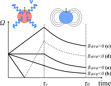
Figure 1: Schematic view of the time evolution of angular velocity, $\Omega$. For $t<\tau_{\nu}$ the neutrino emission changes the NS spin and for $\tau_{\nu}<t<\tau_{0}$ the NS rotation is decelerated by the usual dipole radiation. Depending on the direction of magnetic fields, the NS spin evolution can be classified as following. In the case (a), since the toroidal filed is absent, for $t<\tau_{\nu}$ the rotation velocity is not altered by neutrino emission; In the case (b), the neutrinos decelerate the NS spin; In the case (c), the neutrinos accelerate the NS spin; In the case (d), the neutrinos first decelerate the NS spin and eventually the NS rotation is stopped. Since the neutrinos transfer the angular momentum even after the NS rotation stops, then the NS starts counterrotating (dotted line). The spin deceleration by dipole radiation does not depend on the rotation direction, so that the spin evolution for $<\tau_{\nu}$ is similar independent on the evolution for $t<\tau_{\nu}$. It is clear that the rotation period of NSs distribute broadly if the neutrinos significantly affect the spin evolution. Therefore, if the neutrino effect dominates the spin evolution of NSs for $t<\tau_{\nu}$, in order to concentrate the current spin period of NSs in a narrow range, neutrino effect upon the NS spin should be small enough.

3 Anisotropic neutrino flux and momentum transfer

3.1 Neutrino transfer equation

Following Arras & Lai (1999a, b), we solve the transfer equation for neutrinos. The Boltzmann equation for neutrinos is given by

$$\frac{1}{c}\frac{\partial f_{\nu}(\vec{p}_{\nu})}{\partial t}+\vec{\Omega}\cdot\nabla f_{\nu}(\vec{p}_{\nu})=S,$$ (1)

where $c$ is the speed of light, $f_{\nu}(\vec{p}_{\nu})$ is the distribution function for neutrinos with momentum $\vec{p}_{\nu}$, $t$ is time, $\vec{\Omega}$ is the propagation direction of neutrinos, and $S$ is the source term, in which scattering and absorption are included.

Since we are considering the neutrino transfer inside a PNS, where the neutrinos propagate diffusely, we employ the following diffusion approximation for the neutrino distribution function,

$$f_{\nu}(\vec{p}_{\nu})=f_{\nu}^{(0)}(\epsilon_{\nu})+g(\epsilon_{\nu})+3\vec{\Omega}\cdot\vec{h}(\epsilon_{\nu}),$$ (2)

where $f^{(0)}_{\nu}$ is the Fermi-Dirac distribution function for neutrinos, $\epsilon_{\nu}$ is the neutrino energy, $g(\epsilon_{\nu})$ is the deviation from thermal equilibrium and $\vec{h}(\epsilon_{\nu})$ is the dipole component that is connected to the neutrino flux.

By averaging Eq. (1) over the whole solid angle and omitting the time derivative term, we get the following moment equation for steady state (Arras & Lai, 1999a)

$$\nabla\left[f_{\nu}^{(0)}+g\right]+\epsilon_{\mathrm{abs}}\kappa_{0}^{\mathrm{abs}}g\hat{B}=-3\kappa_{0}^{\mathrm{tot}}\vec{h},$$ (3)

where $\epsilon_{\mathrm{abs}}$ is a coefficient related to absorption and originates from the existence of strong magnetic fields (if there are no magnetic fields $\epsilon_{\mathrm{abs}}$ is zero). $\kappa^{\mathrm{abs}}_{0}$ is the inverse of the mean free path for neutrino emission and absorption ($p+e^{-}\rightleftharpoons n+\nu_{e}$) and $\kappa^{\mathrm{tot}}_{0}$ is the inverse of the mean free path for all interactions, including isoenergetic scattering by nucleons without magnetic fields. Lastly, $\hat{B}\equiv\vec{B}/|\vec{B}|$.

Similarly, we obtain the first order moment equation by integrating Eq. (1) multiplied by $\mu=\vec{\Omega}\cdot\vec{r}/|\vec{r}|$ as

$$\nabla\cdot\vec{h}=-\kappa_{0}^{\mathrm{abs}}g-\epsilon_{\mathrm{abs}}\kappa_{0}^{\mathrm{abs}}\vec{h}\cdot\hat{B}.$$ (4)

Note that to obtain Eqs. (3) and (4) we omitted source terms relating to the scattering originating from the existence of magnetic fields (denoted $\epsilon_{\mathrm{sc}}$ in Arras & Lai 1999a, b). This is because this contribution is much smaller that from the terms proportional to $\epsilon_{\mathrm{abs}}$.

Combining Eqs. (3) and (4), we get the following diffusion equation

$$\frac{1}{3r^{2}}\frac{\partial}{\partial r}\left[\frac{r^{2}}{\kappa_{0}^{\mathrm{tot}}}\frac{\partial(f_{0}+g)}{\partial r}\right]=\kappa_{0}^{\mathrm{abs}}g.$$ (5)

Note that we omitted the higher-order term proportional to $\epsilon_{\mathrm{abs}}^{2}$. Using the specified opacities for $\kappa^{\mathrm{abs}}_{0}$ and $\kappa^{\mathrm{tot}}_{0}$, we can solve this diffusion equation.

Following (Arras & Lai, 1999b), the opacities are estimated as:

$$\kappa^{\mathrm{abs}}_{0}(\epsilon_{\nu})= \frac{(G_{F}\hbar c)^{2}}{\pi}(\epsilon_{\nu}+Q)^{2}n_{n}(c_{V}^{2}+3c_{A}^{2})\left[1-f_{e}(\epsilon_{\nu}+Q)\right]$$

$$= 3.66\times 10^{-9}~{}\mathrm{cm}^{-1}\left(\frac{\epsilon_{\nu}+Q}{2.29~{}\mathrm{MeV}}\right)^{2}\left(\frac{\rho}{10^{11}~{}\mathrm{g~{}cm^{-3}}}\right)$$

$$\times\left[1-f_{e}(\epsilon_{\nu}+Q)\right],$$ (6)

$$\kappa^{\mathrm{sc}}_{0}(\epsilon_{\nu}) =\frac{2}{3\pi}(G_{F}\hbar c)^{2}\epsilon_{\nu}^{2}\left(c_{V}^{2}+5c_{A}^{2}\right)n$$

$$=3.38\times 10^{-10}~{}\mathrm{cm}^{-1}\left(\frac{\epsilon_{\nu}}{1~{}\mathrm{MeV}}\right)^{2}\left(\frac{\rho}{10^{11}~{}\mathrm{g~{}cm^{-3}}}\right),$$ (7)

$$\kappa^{\mathrm{tot}}_{0}(\epsilon_{\nu}) =\kappa^{\mathrm{abs}}_{0}(\epsilon_{\nu})+\kappa^{\mathrm{sc}}_{0}(\epsilon_{\nu}).$$ (8)

Here, $G_{F}=1.166\times 10^{-5}$ GeV^-2 is Fermi’s constant, $\hbar=1.054\times 10^{-27}$ cm² g s^-1 is the reduced Planck constant, $Q=1.29$ MeV is the difference in mass between a neutron and proton, $n_{n}$ is the number density of neutrons, $c_{V}$ and $c_{A}$ are weak interaction constants, $f_{e}$ is the distribution function for electrons and $n$ is the number density of nucleons. For deriving typical values we used $n_{n}=n_{p}=n/2$, where $n_{p}$ is the number density of protons. The composition is assumed to be completely dissociated to free protons and neutrons. We have neglected stimulated absorption effects for simplicity.

The absorption coefficient, as given by Arras & Lai (1999b), is

$$\epsilon_{\mathrm{abs}} =\frac{1}{2}\frac{(\hbar c)^{2}eB}{(\epsilon_{\nu}+Q)^{2}}\frac{c_{V}^{2}-c_{A}^{2}}{c_{V}^{2}+3c_{A}^{2}}$$ (9)

$$=-0.0575\left(\frac{B}{10^{15}~{}\mathrm{G}}\right)\left(\frac{\epsilon_{\nu}+Q}{2.29~{}\mathrm{MeV}}\right)^{-2},$$ (10)

where $c_{V}=1$, and $c_{A}=1.26$ for absorption.

The density profile employed in this study, which mimics the structure of the protoneutron star, is

$$\rho(r)=\rho_{\nu}\left(\frac{r}{R_{\nu}}\right)^{-3},$$ (11)

where $\rho_{\nu}$ is the density of the PNS surface and $R_{\nu}$ is the radius of the protoneutron star. Here we take $\rho_{\nu}=10^{11}$ g cm^-3 and $R_{\nu}=100$ km. Although the density diverges at the center, it does not matter in this study because neutrinos are tightly coupled with matter and $f_{\nu}=f^{(0)}_{\nu}$ there.

By assuming that the matter temperature is constant and neutrinos are not degenerated (i.e. taking the chemical potential of neutrinos to be vanishing), we obtain the following steady state equation for $G\equiv g/f^{(0)}_{\nu}$

$$G^{\prime\prime}+\frac{5}{r}G^{\prime}-\alpha\left(\frac{R_{\nu}}{r}\right)^{6}G=0,$$ (12)

where a prime denotes the derivative with respect to $r$ and

$$\alpha= 4.01\times 10^{-17}\mathrm{cm}^{-2}\left(\frac{\epsilon_{\nu}+Q}{2.29~{}\mathrm{MeV}}\right)^{4}\left(1-f_{e}\right)^{2}$$

$$+3.71\times 10^{-18}\mathrm{cm}^{-2}\left(\frac{\epsilon_{\nu}+Q}{2.29~{}\mathrm{MeV}}\right)^{2}\left(\frac{\epsilon_{\nu}}{1~{}\mathrm{MeV}}\right)^{2}$$

$$\times\left(1-f_{e}\right).$$ (13)

The solution to Eq. (12) is given by

$$G=C_{1}\frac{I_{1}(\sqrt{\alpha}R_{\nu}^{3}/2r^{2})}{r^{2}}+C_{2}\frac{K_{1}(\sqrt{\alpha}R_{\nu}^{3}/2r^{2})}{r^{2}},$$ (14)

where $I$ and $K$ denote modified Bessel functions of the first and second kind, respectively, and $C_{1}$ and $C_{2}$ are constants. At the center, neutrinos are tightly coupled with matter so that $f_{\nu}=f^{(0)}_{\nu}$ and $g=0$, meaning that $C_{1}=0$. From Eq. (3), the flux is given as

$$\vec{h}=-\frac{1}{3\kappa_{0}^{\mathrm{tot}}}\left(G^{\prime}f_{\nu}^{(0)}\hat{r}+\epsilon_{\mathrm{abs}}\kappa_{0}^{\mathrm{abs}}Gf_{\nu}^{(0)}\hat{B}\right),$$ (15)

where $\hat{r}$ denotes the unit vector in the radial direction. Since the specific neutrino flux is given by $\vec{F}_{\nu}=(\epsilon_{\nu}/2\pi\hbar c)^{3}c\vec{h}$, $r-$ and $\phi-$components are given as

$$F^{r}_{\nu} =-\frac{c}{3\kappa_{0}^{\mathrm{tot}}}\left(\frac{\epsilon_{\nu}}{2\pi\hbar c}\right)^{3}\left(G^{\prime}+\epsilon_{\mathrm{abs}}\kappa_{0}^{\mathrm{abs}}G\frac{B^{r}}{B}\right)f_{\nu}^{(0)},$$ (16)

$$F^{\phi}_{\nu} =-\frac{c}{3\kappa_{0}^{\mathrm{tot}}}\left(\frac{\epsilon_{\nu}}{2\pi\hbar c}\right)^{3}\epsilon_{\mathrm{abs}}\kappa_{0}^{\mathrm{abs}}G\frac{B^{\phi}}{B}f^{(0)}_{\nu}.$$ (17)

Here, $B^{r}$ and $B^{\phi}$ correspond to the $r-$ and $\phi-$components of the magnetic field, respectively. $F^{r}_{\nu}$ should be positive at $R_{\nu}$ so that $C_{2}<0$.

By integrating over energy, using the matter temperature $kT=4$ MeV and vanishing chemical potentials for $f^{(0)}_{\nu}$ and $f_{e}$, the ratio between fluxes in the radial and orthogonal directions at the neutrinosphere surface is given by

$$\left.\frac{\int d\epsilon_{\nu}F^{\phi}_{\nu}}{\int d\epsilon_{\nu}F^{r}_{\nu}}\right|_{r=R_{\nu}}\approx-0.013\left(\frac{B^{\phi}}{10^{15}~{}\mathrm{G}}\right)\left(\frac{R_{\nu}}{100~{}\mathrm{km}}\right)^{1/2}.$$ (18)

The second term in Eq. (16) is neglected in this estimation.

The total neutrino luminosity is given by

$$L_{\nu}=\int d\epsilon_{\nu}d\Omega F^{r}_{\nu}R_{\nu}^{2},$$ (19)

and the rate of angular momentum transfer by neutrinos is given by

$$J_{\nu}=\frac{1}{c}\int d\epsilon_{\nu}d\Omega F^{\phi}_{\nu}R_{\nu}^{3}\sin\theta.$$ (20)

The factor $R_{\nu}\sin\theta$ comes from the distance from the symmetry axis. By combining Eqs. (18), (19) and (20), and assuming that $F^{r}_{\nu}$ is independent of the angle, we obtain

$$J_{\nu}= -0.013\left(\frac{\left<B^{\phi}\right>}{10^{15}~{}\mathrm{G}}\right)\left(\frac{R_{\nu}}{100~{}\mathrm{km}}\right)^{1/2}\frac{R_{\nu}L_{\nu}}{c}$$ (21)

$$= -4.3\times 10^{47}~{}\mathrm{g~{}cm^{2}~{}s^{-2}}$$

$$\times\left(\frac{\left<B^{\phi}\right>}{10^{15}~{}\mathrm{G}}\right)\left(\frac{R_{\nu}}{100~{}\mathrm{km}}\right)^{3/2}\left(\frac{L_{\nu}}{10^{53}~{}\mathrm{erg~{}s^{-1}}}\right),$$ (22)

where $\left<B^{\phi}\right>\equiv\int d\Omega B^{\phi}\sin\theta/4\pi$, which is the angle-averaged strength.

3.2 Angular momentum transfer by neutrinos

In this subsection we evaluate the angular momentum transferred by the anisotropic neutrino radiation that interacts with the toroidal magnetic field. This process occurs during the PNS cooling phase when the neutrino diffusion approximation is valid in the stellar interior (Section 3.1). By comparing it with the total angular momentum of a rotating NS, we are able to determine an expression for the critical magnetic field strength at which the NS rotation period is drastically affected by the anisotropic neutrino radiation. In order to compare with present observations, here we employ the NS angular momentum at a stellar radius of 10 km after the PNS cooling phase. This assumption is valid if the angular momentum is conserved when the PNS (i.e. hot NS) contracts to a cold NS, where the radius shrinks from $\sim$100 km to $\sim$10 km.

The angular momentum of a NS is written as

$$\mathcal{M}_{\mathrm{NS}}^{\phi} =I\Omega$$

$$=7.0\times 10^{45}~{}\mathrm{g~{}cm^{2}~{}s^{-1}}\left(\frac{P}{1~{}\mathrm{s}}\right)^{-1}\left(\frac{M}{1.4M_{\odot}}\right)\left(\frac{R_{\mathrm{NS}}}{10~{}\mathrm{km}}\right)^{2},$$ (23)

where $I=\frac{2}{5}MR^{2}_{\mathrm{NS}}$ is the moment of inertia, $\Omega$ is the angular velocity, $P$ is the rotation period ($P=2\pi/\Omega$), $M$ is the NS mass and $R_{\mathrm{NS}}$ is the NS radius.

The angular momentum transferred by neutrino radiation is given by

$$\mathcal{M}_{\nu}^{\phi} =\beta\frac{R_{\nu}E_{\nu}}{c}$$

$$=6.7\times 10^{48}~{}\mathrm{g~{}cm^{2}~{}s^{-1}}\beta\left(\frac{R_{\nu}}{100~{}\mathrm{km}}\right)\left(\frac{E_{\nu}}{2\times 10^{52}~{}\mathrm{erg}}\right),$$ (24)

where $\beta$ is the asymmetry parameter for neutrino emission and $E_{\nu}$ is the total energy emitted by the neutrinos responsible for the change in spin, which is related to the luminosity as $E_{\nu}=\int dtL_{\nu}$. Note that a PNS has larger radius than an ordinary NS due to the existence of thermal pressure (see e.g. Janka, 2012; Suwa et al., 2013). Although the total amount of energy that can be released by the neutrinos is $\sim 3\times 10^{53}$ erg, the contributions from $\nu_{\mu}$ ($\nu_{\tau}$) and $\bar{\nu}_{\mu}$ ($\bar{\nu}_{\tau}$) to the change in spin cancel each other (Arras & Lai, 1999b). As such, we only consider the energy released due to the $\nu_{e}$ emitted in electron capture ($p+e\to n+\nu_{e}$) just after the core bounce of supernova shock, which is $\sim O(10^{52})$ erg. The total number of $\nu_{e}$ emitted due to electron capture is estimated as

$$N_{\nu_{e}}=N_{p}=\frac{MY_{p}}{m_{p}}=8.3\times 10^{56}\left(\frac{M}{1.4M_{\odot}}\right)\left(\frac{Y_{p}}{0.5}\right),$$ (25)

where $N_{p}$ is the total number of protons in the neutron star, $m_{p}$ is the proton mass and $Y_{p}$ is the proton fraction. By taking the average energy of emitted $\nu_{e}$ to be 3.15$kT=12.6$ MeV ($kT$/4 MeV), the total energy released due to $\nu_{e}$ emission in the neutralization process is given as $E_{\nu_{e}}=1.7\times 10^{52}~{}\mathrm{erg}(M/1.4M_{\odot})(Y_{p}/0.5)(kT/4~{}\mathrm{MeV})$.

Comparing Eqs. (23) and (24), one recognizes that the slowly rotating ($P\sim 1$ s) PNS’s rotation can be significantly affected if $\beta\sim 10^{-3}$. This condition can be used to put a constraint on the strength of internal toroidal magnetic fields. From Eqs. (22) and (24), $\beta$ is given as

$$\beta\approx-0.013\left(\frac{\left<B^{\phi}\right>}{10^{15}~{}\mathrm{G}}\right)\left(\frac{R_{\nu}}{100~{}\mathrm{km}}\right)^{1/2},$$ (26)

where we have used $\int dtL_{\nu}=E_{\nu}$. Using these relations, in the next section we will constrain the internal toroidal field.

4 Constraint on Internal Toroidal Fields

It is natural to expect that the angular momentum transferred by neutrinos should be smaller than the total angular momentum of the PNS at $t=\tau_{\nu}$ (see Section 2). As such, using Eqs. (23) and (24) we get the following constraint:

$$|\beta|\mathrel{\hbox{\hbox to0.0pt{\hbox{\lower 5.0pt\hbox{$\sim$}}\hss}\hbox{$<$}}} 1.0\times 10^{-3}\left(\frac{P}{1~{}\mathrm{s}}\right)^{-1}\left(\frac{M}{1.4M_{\odot}}\right)\left(\frac{R_{\mathrm{NS}}}{10~{}\mathrm{km}}\right)^{2}$$

$$\times\left(\frac{R_{\nu}}{100~{}\mathrm{km}}\right)^{-1}\left(\frac{E_{\nu}}{2\times 10^{52}~{}\mathrm{erg}}\right)^{-1},$$ (27)

which can be rewritten as a constraint on the magnetic fields using Eq. (26) as

$$\left|\left<B^{\phi}\right>\right|\mathrel{\hbox{\hbox to0.0pt{\hbox{\lower 5.0pt\hbox{$\sim$}}\hss}\hbox{$<$}}} 8.1\times 10^{13}~{}\mathrm{G}\left(\frac{P}{1~{}\mathrm{s}}\right)^{-1}\left(\frac{M}{1.4M_{\odot}}\right)\left(\frac{R_{\mathrm{NS}}}{10~{}\mathrm{km}}\right)^{2}$$

$$\times\left(\frac{R_{\nu}}{100~{}\mathrm{km}}\right)^{-3/2}\left(\frac{E_{\nu}}{2\times 10^{52}~{}\mathrm{erg}}\right)^{-1}.$$ (28)

By exploiting the fact that the magnetic flux is conserved during the PNS cooling phase, i.e. $\left<B_{\mathrm{NS}}^{\phi}\right>R_{\mathrm{NS}}^{2}=\left<B^{\phi}\right>R_{\nu}^{2}$, we can evaluate the field strength inside a cold NS whose radius is $R_{\mathrm{NS}}$ as

$$\left|\left<B_{\mathrm{NS}}^{\phi}\right>\right|\mathrel{\hbox{\hbox to0.0pt{\hbox{\lower 5.0pt\hbox{$\sim$}}\hss}\hbox{$<$}}} 8.1\times 10^{15}~{}\mathrm{G}\left(\frac{P}{1~{}\mathrm{s}}\right)^{-1}\left(\frac{M}{1.4M_{\odot}}\right)$$

$$\times\left(\frac{R_{\nu}}{100~{}\mathrm{km}}\right)^{1/2}\left(\frac{E_{\nu}}{2\times 10^{52}~{}\mathrm{erg}}\right)^{-1}.$$ (29)

We therefore see that the constraint on the magnetic field strength depends on the rotation period $P$ at $t=\tau_{\nu}$. The typical spin period of magnetars at $t=\tau_{\nu}$ is unclear due to the lack of knowledge on magnetar formation. However, if we take $P=10$ ms at $t=\tau_{\nu}$, we obtain $\left|\left<B_{\mathrm{NS}}^{\phi}\right>\right|\mathrel{\hbox{\hbox to0.0pt{\hbox{\lower 5.0pt\hbox{$\sim$}}\hss}\hbox{$<$}}}10^{18}$ G.

If we assume that magnetic dipole radiation is the dominant process affecting magnetar spin evolution for $t>\tau_{\nu}$, the spin period of 1E 1841-045 at $t=\tau_{\nu}$ can be estimated as $\approx$ 8-11 s (see Appendix A). Therefore, using Eq. (29), we can obtain the following constraint on the field strength:

$$\left|\left<B_{\mathrm{NS}}^{\phi}\right>\right|\mathrel{\hbox{\hbox to0.0pt{\hbox{\lower 5.0pt\hbox{$\sim$}}\hss}\hbox{$<$}}}10^{15}~{}\mathrm{G}\left(\frac{R_{\nu}}{100~{}\mathrm{km}}\right)^{1/2},$$ (30)

where we have employed canonical values for $M$ and $E_{\nu}$. A similar value is obtained for the case of 1E 2259+586. Thus, the toroidal magnetic fields of these magnetars can be comparable to the dipole component at least at the moment of birth. Note that this constraint only applies to the global toroidal field, i.e. the angle averaged value near the NS surface, since the angular momenta transferred by turbulent components on small scales cancel each other out.

5 Summary and Discussion

In this paper we studied the spin evolution of magnetars resulting from the anisotropic neutrino emission induced by strong magnetic fields. We solved the diffusion equation for neutrinos and estimated the degree of anisotropy. By considering the toroidal component of the magnetic fields we were able to constrain the unseen internal fields using the current rotation period of magnetars. Supposing that the associated SNR age is the real magnetar age, we found the constraint $\left|\left<B^{\phi}_{\mathrm{NS}}\right>\right|\mathrel{\hbox{\hbox to0.0pt{\hbox{\lower 5.0pt\hbox{$\sim$}}\hss}\hbox{$<$}}}10^{15}$ G for 1E1841-045 and 1E 2259+586, whose dipole fields are thought to be $\sim 10^{15}$ G and $10^{14}$ G, respectively.

In addition to the spin evolution, we can also estimate the pulsar kick velocity of magnetars using Eq. (18). When we consider the split monopole poloidal field at the PNS surface, the degree of asymmetry $\gamma$ is $O(10^{-2})(B_{p}/10^{15}~{}\mathrm{G})$. The kick velocity can thus be estimated as

$$v_{\mathrm{kick}} =\gamma\frac{E_{\nu}}{Mc}$$ (31)

$$\approx 24.0~{}\mathrm{km~{}s^{-1}}\left(\frac{\gamma}{10^{-2}}\right)\left(\frac{E_{\nu}}{2\times 10^{52}~{}\mathrm{erg}}\right)\left(\frac{M}{1.4M_{\odot}}\right)^{-1}.$$ (32)

We therefore see that the magnetar kick resulting from this mechanism is expected to be very small.

In this paper we focused on magnetars (SGRs and AXPs). However, there are other classes of stars that also have strong dipole fields (see Dall’Osso et al., 2012, for a list). These objects exhibit a similar spin period to magnetars (3 s $\mathrel{\hbox{\hbox to0.0pt{\hbox{\lower 5.0pt\hbox{$\sim$}}\hss}\hbox{$<$}}}P\mathrel{\hbox{\hbox to0.0pt{\hbox{\lower 5.0pt\hbox{$\sim$}}\hss}\hbox{$<$}}}$ 11 s), but their magnetic fields are typically weaker. Even though they do not have associated SNR, we can apply the same analysis as discussed in this paper taking $P_{i}\sim O(1)$ s. Thus, the constraint obtained in this study is applicable for these objects as well as magnetars.

To finish we comment on the assumptions made in this study. First, we employed the diffusion approximation for the neutrino radiative transfer equation. This assumption is essentially valid for the region of the magnetar considered in this work, but near the surface, where the mean free path of neutrinos is comparable to the scale size, this approximation starts to break down. However, since we are considering the region inside the PNS, the effect of the break-down of this assumption is not significant. Secondly, for simplicity we have assumed that the PNS radius is constant during the cooling phase. However, this assumption does not change our discussion drastically because the constraints on the internal toroidal magnetic field given by Eqs. (29) and (30) imply very weak dependence on the PNS radius. In addition, since a smaller PNS radius gives a tighter upper limit for the toroidal field, our assumption of constant radius will tend to give more conservative upper limits. Thirdly, since the real age of a magnetar is unknown, we assumed it to be the same as that of the SNR. Because the SNR age contains systemic errors, this approximation might affect the derived constraint. However, we expect that the corrections to the age do not change it by orders of magnitude, meaning that our discussion in the previous section should not change very much even if we include this systematic error. Finally, we have assumed that after neutrino emission the sole mechanism behind the magnetar spin-down is dipole radiation. There are several other mechanisms that can decelerate a NS’s spin (see e.g. Thompson et al., 2004), which will tend to lead to looser constraints on the internal fields. This is because these mechanisms usually act later than the neutrinos so that a smaller $P_{i}$ is possible. More detailed studies that include the effects of other deceleration mechanisms are necessary. A fundamental limit can be obtained using the fastest rotation of a NS (i.e. the rotational breakup speed), which gives $\left<B^{\phi}_{\mathrm{NS}}\right>\mathrel{\hbox{\hbox to0.0pt{\hbox{\lower 5.0pt\hbox{$\sim$}}\hss}\hbox{$<$}}}10^{19}$ G.

Appendix A Spin evolution of magnetars

A.1 Case without magnetic field decay

Since the real age of a magnetar, $\tau_{0}$, is unknown, the characteristic spin-down time, $\tau_{c}\equiv P/2\dot{P}$, is conventionally used as an approximation. We also know that some magnetars can be associated with SNRs, for which alternative, better age estimations are possible via X-ray plasma diagnostics. Here we assume that the SNR age is a better estimator of $\tau_{0}$, and extrapolate the current rotation period to the initial period at $\tau_{\nu}$ using the dipole radiation model. In the following discussion we give expressions for the initial rotation period $P_{i}$ at $\tau_{\nu}$ and its evolution. In this subsection we neglect the magnetic field decay, which will be discussed in the next subsection.

When dipole radiation is the leading cause of spin-down, the rotation period as a function of time, $t$, can be written as (Shapiro & Teukolsky, 1983)

$$P=P_{i}\left(1+\frac{2P^{2}}{P_{i}^{2}}\frac{t}{T}\right)^{1/2},$$ (33)

where the initial period, $P_{i}$, at $t=\tau_{\nu}$ is given at the time when dipole radiation becomes the dominant process for spin down and

$$T= \frac{P}{\dot{P}}=\frac{3Ic^{3}P^{2}}{2\pi^{2}B_{p}^{2}R^{6}\sin^{2}\alpha}$$ (34)

$$= 145~{}\mathrm{years}\left(\frac{B_{p}}{10^{15}~{}\mathrm{G}}\right)^{-2}\left(\frac{R}{10~{}\mathrm{km}}\right)^{-4}\left(\frac{M}{1.4M_{\odot}}\right)\left(\frac{P}{1~{}\mathrm{s}}\right)^{2},$$ (35)

where $B_{p}$ is the surface dipole field at the pole. Here we employ $\sin^{2}\alpha=1$ for simplicity. Using this relation we find

$$B_{p} =\left(\frac{3Ic^{3}}{2\pi^{2}R^{6}}P\dot{P}\right)^{1/2}$$

$$=6.75\times 10^{19}~{}\mathrm{G}\left(\frac{M}{1.4M_{\odot}}\right)\left(\frac{R}{10~{}\mathrm{km}}\right)^{-4}\left(\frac{P}{1~{}\mathrm{s}}\right)^{1/2}\left(\frac{\dot{P}}{1~{}\mathrm{s/s}}\right)^{1/2}.$$ (36)

Although this result looks different by a factor of two to the frequently used $B=3.2\times 10^{19}~{}\mathrm{G}\sqrt{P\dot{P}}$, this difference just comes from a difference in notation. By substituting Eq. (34) into (33), we get the following simple form as

$$P^{2}=P_{i}^{2}+\frac{4\pi^{2}B_{p}^{2}R^{6}\sin^{2}\alpha}{3Ic^{3}}t.$$ (37)

In Figure 2 we show the evolution of the spin period of neutron stars with various strengths of the constant dipole field. The red crosses correspond to observed magnetars for which the characteristic age is used ($\tau_{c}\equiv P/2\dot{P}$), whilst the blue points correspond to magnetars that can be associated with SNRs, so that the SNR age is used. For $B_{p}=10^{15}$ G we plot the evolution for two different initial periods ($P_{i}$=1 s for the top line and 1 ms for the bottom line). One finds that the evolutions coincide after $\mathrel{\hbox{\hbox to0.0pt{\hbox{\lower 5.0pt\hbox{$\sim$}}\hss}\hbox{$>$}}}$ 1000 years, from which we conclude that $P_{i}$ does not affect the late time evolution.

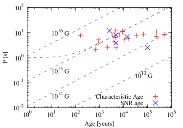
Figure 2: The time evolution of rotation period for NSs with different dipole magnetic fields (grey dashed lines). The imposed magnetic field strengths are shown near the corresponding lines. Red and blue points indicate the observational data for which characteristic ages ($\tau_{c}=P/2\dot{P}$) and SNR ages are used, respectively. For $B_{p}=10^{15}$ G we plot two lines with different initial periods. The top and bottom lines correspond to initial periods of 1 s and 1 ms, respectively.

As can be seen in Table 1, there are two magnetars for which the SNR age is younger than the characteristic age. For example, 1E 2259+586 and associated SNR CTB 109 exhibit a large discrepancy between the two ages. Here we treat the SNR age as the true age and use this to estimate the spin periods of the magnetars at birth. In Figure 3 we show the time evolution of the spin period for values of $P$ and $\dot{P}$ equal to those of 1E 1841-045. We find that $P_{i}$ should be $\approx$ 8–11 s in order to explain the current observation with the age of $\sim$1 kyr. The same analysis also gives the initial period of 1E 2259+586 as $P_{i}\approx 7$ s, which is almost the same as the current period. Note that these values would be smaller if decay of the poloidal magnetic field were included, which will be discussed in the next subsection.

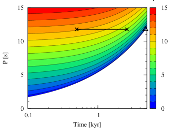
Figure 3: Period evolution with time for NSs with values of $P$ and $\dot{P}$ equal to those of 1E 1841-045. The black contour lines correspond to trajectories with different initial spin periods, $P_{i}$. The value of $P_{i}$ can be read off from the color map. The thick horizontal black line represents the SNR age including systematic errors as given in Tian & Leahy (2008), with the two crosses marking the lower and upper limits of 0.5 kyr and 2.6 kyr, respectively. In order to explain observational data, $P_{i}\approx$ 8–11 s is necessary. The triangle corresponds to the characteristic age ($\approx$ 4.8 kyr), and lies on a trajectory with infinitely small $P_{i}$.

A.2 Case with magnetic field decay

In this subsection we study spin evolution including phenomenologically the effect of magnetic field decay. It is important to consider the effect of the decaying magnetic field because there is no isolated NS with $P\mathrel{\hbox{\hbox to0.0pt{\hbox{\lower 5.0pt\hbox{$\sim$}}\hss}\hbox{$>$}}}12$ s, meaning that the dipole radiation can be assumed to become small enough so as to not affect the spin period for slowly rotating NSs. There are several studies that investigate the long-term evolution of magnetic fields including their decay (e.g., Colpi et al., 2000; Dall’Osso et al., 2012; Nakano et al., 2012; Pons et al., 2013).

Using the model of Colpi et al. (2000) and Dall’Osso et al. (2012), after several algebraic steps we get the following expressions for the time evolution of the spin period and the dipole magnetic field strength:

$$P^{2}(t) =P_{\infty}^{2}-(P_{\infty}^{2}-P_{i}^{2})\left(1+\frac{t}{\tau_{d}}\right)^{(\alpha_{B}-2)/\alpha_{B}},$$ (38)

$$B_{p}(t) =\frac{B_{i}}{(1+t/\tau_{d})^{1/\alpha_{B}}},$$ (39)

where $P_{\infty}$ is the final spin period, $\tau_{d}$ is the decay timescale of the magnetic fields, $\alpha_{B}$ is a parameter describing the magnetic field decay and $B_{i}$ is the initial magnetic field strength. In Dall’Osso et al. (2012) it was found that models with $1.5\mathrel{\hbox{\hbox to0.0pt{\hbox{\lower 5.0pt\hbox{$\sim$}}\hss}\hbox{$<$}}}\alpha_{B}\mathrel{\hbox{\hbox to0.0pt{\hbox{\lower 5.0pt\hbox{$\sim$}}\hss}\hbox{$<$}}}1.8$ can explain most of the observational evidence for isolated neutron stars with strong magnetic fields (not only magnetars but also X-ray dim isolated NSs). Although $P_{\infty}$ is unknown, Dall’Osso et al. (2012) and Pons et al. (2013) suggested that $P_{\infty}\approx 12$ s, because there is no observed NS with $P\mathrel{\hbox{\hbox to0.0pt{\hbox{\lower 5.0pt\hbox{$\sim$}}\hss}\hbox{$>$}}}12$ s. Thus, we employ $P_{\infty}=12$ s as a fiducial value here. In addition, Dall’Osso et al. (2012) showed that taking $10^{15}~{}\mathrm{G}\mathrel{\hbox{\hbox to0.0pt{\hbox{\lower 5.0pt\hbox{$\sim$}}\hss}\hbox{$<$}}}B_{i}\mathrel{\hbox{\hbox to0.0pt{\hbox{\lower 5.0pt\hbox{$\sim$}}\hss}\hbox{$<$}}}10^{16}~{}\mathrm{G}$ gives good agreement with the distribution of observed NSs with strong magnetic fields in the $\tau_{c}$-$B_{p}$ plane. We thus use $B_{i}=10^{16}$ G in the following. In order to explain observed features, Dall’Osso et al. (2012) suggested that $\tau_{d}=$1 kyr/$(B_{i}/10^{15}~{}\mathrm{G})^{\alpha_{B}}$.

In Figure 4 we show the period evolution of magnetars as determined using the decaying magnetic field model. In this figure the top axis gives the strength of poloidal field (decreasing from the initial value of $10^{16}$ G). The blank square shows the current position of 1E1841-045 in the $P$-$B_{p}$ plane, as estimated from $P$ and $\dot{P}$. We see that the square overlaps with the left-hand cross, which corresponds to the lower limit on the SNR age. As such, this model can be used to consistently explain all three observed quantities $P$, $B_{p}$ and the SNR age. One can see that $P_{i}\mathrel{\hbox{\hbox to0.0pt{\hbox{\lower 5.0pt\hbox{$\sim$}}\hss}\hbox{$>$}}}11$ s is still required in order to explain observations using the decaying magnetic field model with fiducial model parameters (case (a)). As such, the discussion in the previous subsection is still valid in this case. We do note, however, that with a fine tuning of the parameters it is possible to explain observational data with $P_{\infty}>12$ s and $P_{i}\ll 1$ s (see case (b)). On the other hand, 1E 2259+586 has $P=6.9789484460$ s. We find that $P_{i}\sim 5$ s by the same discussion with fiducial parameters, which is similar value as 1E 1841-045. Therefore, even with the decaying magnetic field model, we find that $P_{i}$ should be $O(1)$ s.

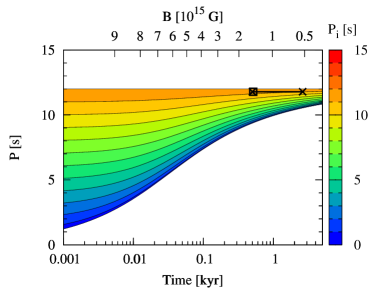
(a) $P_{\infty}=12$ s

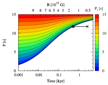
(b) $P_{\infty}=15$ s

Figure 4: The same as Fig. 3 but for the decaying magnetic field model (see Eqs. 38 and 39) with the initial magnetic field $B_{i}=10^{16}$ G. The top axis corresponds to the strength of poloidal dipole magnetic field (see Eq. 39). The left panel is for $P_{\infty}=12$ s and the right panel for $P_{\infty}=15$ s. The blank square marks the current observed $B_{p}$ and $P$, and is almost coincident with the left-hand cross that marks the lower limit on the SNR age.

Table 1: Observational properties of SGRs and AXPs

SGR/AXP name†	$P$ [s]	$\dot{P}$ [$10^{-11}$ s/s]	$B_{p}$ [$10^{14}$ G]‡	$\tau_{c}$ [kyr]§	SNR age [kyr]
SGR 0418+5729	9.07838827(4)	$<$0.0006	$<$0.16	$2.4\times 10^{4}<$	—
SGR 0501+4516	5.76209653(3)	0.582(3)	3.9	16	—
SGR 0526-66	8.0544(2)	3.8(1)	12	3.4	4.8¶
SGR 1627-41	2.594578(6)	1.9(4)	4.7	2.2	—
SGR 1806-20	7.6022(7)	75(4)	51	0.16	—
Swift J1822.3-1606	8.43771977(4)	0.0254(22)	0.99	530	—
SGR 1833-0832	7.5654084(4)	0.35(3)	3.5	34	—
Swift J1834.9-0846	2.4823018(1)	0.796(12)	3.0	4.9	60–200#
SGR 1900+14	5.19987(7)	9.2(4)	15	0.90	—
CXOU J010043.1-721134	8.020392(9)	1.88(8)	8.3	6.8	—
4U 0142+61	8.68832877(2)	0.20332(7)	2.8	68	—
1E 1048.1-5937	6.457875(3)	$\sim$2.25	8.1	4.5	—
1E 1547.0-5408	2.0721255(1)	$\sim$4.7	6.7	0.70	N/A
PSR J1622-4950	4.3261(1)	1.7(1)	5.8	4.0	—
CXO J164710.2-455216	10.6106563(1)	$\sim$0.073	1.9	230	—
1RXS J170849.0-400910	11.003027(1)	1.91(4)	9.8	9.1	—
CXOU J171405.7-381031	3.82535(5)	6.40(14)	11	0.95	4.9%
XTE J1810-197	5.5403537(2)	0.777(3)	4.4	11	—
1E 1841-045	11.7828977(10)	3.93(1)	15	4.8	0.5–2.6&
1E 2259+586	6.9789484460(39)	0.048430(8)	1.2	230	14$

^†Data taken from McGill SGR/AXP Online Catalog (Olausen & Kaspi, 2014) (see also Viganò et al. 2013).

^‡The estimation is based on Eq. (36).

^§Characteristic ages estimated as $P/2\dot{P}$.

^¶Park et al. (2012).

^#Tian et al. (2007).

^%Aharonian et al. (2008).

^&Tian & Leahy (2008).

^$Sasaki et al. (2013).

References

- Aharonian et al. (2008) Aharonian, F., Akhperjanian, A. G., Barres de Almeida, U., et al. 2008, A&A, 486, 829
- Ando (2003) Ando, S. 2003, Phys. Rev. D, 68, 063002
- Arras & Lai (1999a) Arras, P., & Lai, D. 1999a, ApJ, 519, 745
- Arras & Lai (1999b) —. 1999b, Phys. Rev. D, 60, 043001
- Burrows & Lattimer (1986) Burrows, A., & Lattimer, J. M. 1986, ApJ, 307, 178
- Colpi et al. (2000) Colpi, M., Geppert, U., & Page, D. 2000, ApJ, 529, L29
- Dall’Osso et al. (2012) Dall’Osso, S., Granot, J., & Piran, T. 2012, MNRAS, 422, 2878
- Enoto et al. (2010) Enoto, T., Nakazawa, K., Makishima, K., Rea, N., Hurley, K., & Shibata, S. 2010, ApJ, 722, L162
- Fischer et al. (2010) Fischer, T., Whitehouse, S. C., Mezzacappa, A., Thielemann, F.-K., & Liebendörfer, M. 2010, A&A, 517, A80
- Janka (2001) Janka, H.-T. 2001, A&A, 368, 527
- Janka (2012) Janka, H.-T. 2012, Annual Review of Nuclear and Particle Science, 62, 407
- Kotake et al. (2005) Kotake, K., Yamada, S., & Sato, K. 2005, ApJ, 618, 474
- Makishima et al. (2014) Makishima, K., Enoto, T., Hiraga, J. S., et al. 2014, Physical Review Letters, 112, 171102
- Maruyama et al. (2014) Maruyama, T., Hidaka, J., Kajino, T., et al. 2014, Phys. Rev. C, 89, 035801
- Maruyama et al. (2012) Maruyama, T., Yasutake, N., Cheoun, M.-K., Hidaka, J., Kajino, T., Mathews, G. J., & Ryu, C.-Y. 2012, Phys. Rev. D, 86, 123003
- Nakano et al. (2012) Nakano, T., Makishima, K., Nakazawa, K., Uchiyama, H., & Enoto, T. 2012, in American Institute of Physics Conference Series, Vol. 1427, American Institute of Physics Conference Series, ed. R. Petre, K. Mitsuda, & L. Angelini, 126–128
- Olausen & Kaspi (2014) Olausen, S. A., & Kaspi, V. M. 2014, ApJS, 212, 6
- Park et al. (2012) Park, S., Hughes, J. P., Slane, P. O., Burrows, D. N., Lee, J.-J., & Mori, K. 2012, ApJ, 748, 117
- Pons et al. (2013) Pons, J. A., Viganò, D., & Rea, N. 2013, Nature Physics, 9, 431
- Rea et al. (2010) Rea, N., et al. 2010, Science, 330, 944
- Rea et al. (2012) —. 2012, ApJ, 754, 27
- Sasaki et al. (2013) Sasaki, M., Plucinsky, P. P., Gaetz, T. J., & Bocchino, F. 2013, A&A, 552, A45
- Shapiro & Teukolsky (1983) Shapiro, S. L., & Teukolsky, S. A. 1983, Black holes, white dwarfs, and neutron stars: The physics of compact objects (New York, Wiley-Interscience, 1983, 663 p.)
- Suwa et al. (2013) Suwa, Y., Takiwaki, T., Kotake, K., Fischer, T., Liebendörfer, M., & Sato, K. 2013, ApJ, 764, 99
- Suwa (2014) Suwa, Y. 2014, PASJ, 66, L1
- Thompson et al. (2004) Thompson, T. A., Chang, P., & Quataert, E. 2004, ApJ, 611, 380
- Tian et al. (2007) Tian, W. W., Li, Z., Leahy, D. A., & Wang, Q. D. 2007, ApJ, 657, L25
- Tian & Leahy (2008) Tian, W. W., & Leahy, D. A. 2008, ApJ, 677, 292
- Tiengo et al. (2013) Tiengo, A., Esposito, P., Mereghetti, S., et al. 2013, Nature, 500, 312
- Trümper et al. (2010) Trümper, J. E., Zezas, A., Ertan, Ü., & Kylafis, N. D. 2010, A&A, 518, A46
- Viganò et al. (2013) Viganò, D., Rea, N., Pons, J. A., et al. 2013, MNRAS, 434, 123