Time dependence of partition into spectators and participants in relativistic heavy-ion collisions

Abstract

The process of formation of the participant system in heavy-ion collisions is investigated in the framework of a simplified analytic Glauber-like model, which is based on the relativistic Boltzmann transport equation. The key point lies in the time-dependent partition of the nucleon system into two groups: nucleons, which did not take part in any interaction before a given time and nucleons, which already have interacted. In the framework of the proposed model we introduce a natural energy-dependent temporal scale $t_{c}$, which allows us to remove all dependencies of the model on the collision energy except for the energy dependence of the nucleon-nucleon cross-section. By investigating the time dependence of the total number of participants we conclude that the formation process of the participant system becomes complete at $t\simeq 1.5t_{c}$. Time dependencies of participant total angular momentum and vorticity are also considered and used to describe the emergence of rotation in the reaction plane.

I Introduction

From the very beginning of the collision of two nuclei some of the nucleons start to experience collisions and become participants. The number of nucleons which have experienced collisions increases with time and the number of the nucleons which did not take part in collisions decreases. Finally, this results in the partition of the total initial system of nucleons into two subsystems: participants and spectators. In the framework of the Glauber model GlauberSitenko ; BialasNWM ; GlauberModel (optical limit) one can obtain average transverse distributions of the participants and spectators at the end of this partition stage. These smooth distributions have been used earlier as input to fluid dynamical models, see e.g., Refs. Kolb2001 ; Kolb2001elliptic . The Monte Carlo Glauber (MC-Glauber) approach allows one to simulate the initial partition stage on an event-by-event level and can be used for determining fluctuating initial conditions in event-by-event hydrodynamics Holopainen2011 ; Schenke2011 ; Qiu2011 . Fluctuations in the collective flow coefficients have been attributed to initial spatial fluctuations Broniowski2007 ; Alver2010 and thus can be used to put constraints on the initial-state geometry Retinskaya2014 ; Renk2014 . On the other hand, fluctuations can develop dynamically during the fluid dynamical motion, especially if the matter undergoes a phase transition K1 ; K2 ; K3 . While the transverse plane distribution (and its fluctuations) of the formed participant system has been investigated in literature in great detail by using the Glauber approach, little attention was paid to the temporal dynamics of the spectator-participant partition. This dynamics can be of special interest in peripheral collisions where one can study, for instance, the process of how participants gain a non-zero total angular momentum, which in turn results in the emergence of initial rotation in the reaction plane. In the present work we develop an analytical Glauber-like model in the framework of the relativistic Boltzmann equation (Sec. II) and use it for the description of the process of partition into spectator and participant subsystems. Calculations done in the model for various time-dependent quantities are presented in Sec. III and conclusions are given in Sec. IV.

II The model

II.1 Initial conditions and the ballistic mode

In the simplest approximation of our description within the relativistic Boltzmann equation we assume a ballistic mode, i.e., we neglect all the reactions between hadrons and we separate the total system of net nucleons into nucleons of the target (A) and projectile (B) nuclei. The initial single-particle distribution functions $f^{(0)}_{A}(x,p)$ and $f^{(0)}_{B}(x,p)$ [hereinafter denoted $f^{(0)}_{A(B)}(x,p)$] of nucleons from corresponding nuclei are described by the collisionless field-free relativistic Boltzmann equation

$$p^{\mu}\partial_{\mu}f^{(0)}_{A(B)}(x,p)\,=\,0\,.$$ (1)

The solution to this equation is

$$f^{(0)}_{A(B)}(x,p)\ =\ \mathcal{F_{A(B)}}\left[\mathbf{r}-\mathbf{v}(t-t_{0}),p\right]\,,$$ (2)

where $\mathcal{F_{A(B)}}(\mathbf{r},p;t_{0})$ is the distribution function of nucleons at the initial time, $t_{0}$, $\mathbf{v}=\mathbf{p}/E_{p}$ is the velocity of particles and $E_{p}=(m^{2}+\mathbf{p}^{2})^{1/2}$. We adopt the system of units $c=\hbar=1$. The initial time, $t_{0}$, corresponds to the moment before any interaction takes place. I.e. no collision and no internal change within the two nuclei occurs between $t=-\infty$ and $t_{0}$.

We assume that the initial distribution function of nucleons in the nucleus can be presented as a product of a spatial and momentum distributions

$$\mathcal{F_{A(B)}}(\mathbf{r},p;t_{0})\,=\,\rho_{A(B)}(\mathbf{r};t_{0})\ g_{A(B)}(\mathbf{p})\ .$$ (3)

Here $\rho_{A(B)}(\mathbf{r};t_{0})$ is the initial spatial distribution of nucleons in the target (projectile), and $g_{A(B)}(\mathbf{p})$ is the initial momentum distribution. Since the collider center-of-mass (c.m.) frame and the Local Rest (LR) frame of a nucleus are connected via the Lorentz transformation in $(t,z)$ variables, we can write the initial spatial density, $\rho_{A(B)}(\mathbf{r};t_{0})$, (which is the 0th component of the nucleon 4-flow) in the collider c.m. system (c.m.s.) in terms of corresponding 4-flow quantities in terms of the Local Rest frame of the nucleus as

$$\rho_{A(B)}(\mathbf{r};t_{0})\,=\,\gamma_{0}\left\{\rho_{A(B)}^{LR}[x,y,\gamma_{0}(z-v_{A(B)}t_{0})]+v_{A(B)}\,j_{z}^{A(B),LR}[x,y,\gamma_{0}(z-v_{A(B)}t_{0})]\right\}\,,$$ (4)

where $v_{A}=-v_{B}=v_{0}$ is the initial nucleus velocity in the c.m. frame, $\gamma_{0}=(1-v_{0}^{2})^{-1/2}$, $\rho_{A(B)}^{LR}(x,y,z)$ is the initial spatial distribution of nucleons in the Local Rest Frame of the target (projectile) nucleus, and $j_{z}^{A(B),LR}(x,y,z)$ is a $z$-coordinate of nucleon flow in the same Local Rest Frame.

For the spatial distribution in the LR frame of the nucleus we use the Woods-Saxon density profile so that

$$\rho_{A(B)}^{LR}(x,y,z)\,=\,\rho_{{}_{WS}}(x\mp b/2,y,z)=c_{\rho}\left\{1+\exp\left[\frac{\sqrt{(x\mp b/2)^{2}+y^{2}+z^{2}}-R_{0}}{a}\right]\right\}^{-1},$$ (5)

where $a=0.545$ fm and $R_{0}$ is the nuclear radius. The normalization constant $c_{\rho}$ is determined from the relation $\int d\mathbf{r}\rho_{{}_{WS}}(\mathbf{r})=A$, where $A$ is the mass number of the nucleus. In the above equation we have already taken into account a shift in the $x$ coordinate due to the non-zero impact parameter $b$. It should be noted that our approach is not restricted just to the standard Woods-Saxon profile, other nuclear density profiles, i.e., three-parameter Woods-Saxon, can also be used. Assuming that the momentum distribution of nucleons in the LR frame of the nucleus is isotropic, we get that the particle flow $j_{z}^{A(B),LR}$ vanishes, and the initial density, $\rho_{A(B)}(\mathbf{r};t_{0})$, in the collider c.m. frame can be written as

$$\rho_{A(B)}(\mathbf{r};t_{0})\,=\,\gamma_{0}\,\rho_{{}_{WS}}[x\mp b/2,y,\gamma_{0}(z-v_{A(B)}t_{0})]\,.$$ (6)

Expression (6) corresponds to nuclear density in the moving frame which has correct normalization, i.e., $\int d\mathbf{r}\,\rho_{A(B)}(\mathbf{r};t_{0})=A$. To define the initial momentum distribution in the c.m. frame we neglect the random Fermi motion in comparison to the collective motion since we are dealing with ultra-relativistic collision energies. In this case the initial momentum distribution, $g_{A(B)}(\mathbf{p})$, reads as

$$g_{A(B)}(\mathbf{p})\ =\ \delta^{2}(\mathbf{p}_{\bot})\,\delta\left(p_{z}-p_{A(B)}\right),$$ (7)

where $p_{A}$ ($p_{B}$) is the initial momentum of nucleons in the target (projectile).

Finally, we write the initial distribution function, $\mathcal{F_{A(B)}}(\mathbf{r},p;t_{0})$, as

$$\mathcal{F_{A(B)}}(\mathbf{r},p;t_{0})\,=\,\gamma_{0}\,\rho_{{}_{WS}}[x\mp b/2,y,\gamma_{0}(z-v_{A(B)}t_{0})]\,\delta^{2}(\mathbf{p}_{\bot})\,\delta\left(p_{z}-p_{A(B)}\right)\ .$$ (8)

We can see that the target and projectile initially move with opposite velocities and they are completely separated spatially at $t=t_{0}$, therefore indicating that the presented initial conditions are consistent with the condition that there are no reactions before the initial time $t_{0}$.

It can be seen that, in this particular case of momentum distribution (7), the expression (8) actually represents a solution of the collision-less Boltzmann equation if we treat $t_{0}$ as the time variable. Indeed, using relation (2) we can write the time-dependent ballistic nucleon distribution functions in collider c.m. as

$$f^{(0)}_{A(B)}(t,\mathbf{r},\mathbf{p}) = \gamma_{0}\,\rho_{{}_{WS}}(x\mp b/2,y,\gamma_{0}[z-\frac{p_{z}}{E_{p}}(t-t_{0})-v_{A(B)}t_{0}])\,\delta^{2}(\mathbf{p}_{\bot})\,\delta\left(p_{z}-p_{A(B)}\right)$$ (9)

$$= \gamma_{0}\,\rho_{{}_{WS}}(x\mp b/2,y,\gamma_{0}[z-v_{A(B)}t])\,\delta^{2}(\mathbf{p}_{\bot})\,\delta\left(p_{z}-p_{A(B)}\right)$$

$$= \frac{\gamma_{0}\,c_{\rho}\,\delta^{2}(\mathbf{p}_{\bot})\,\delta\left(p_{z}-p_{A(B)}\right)}{1+\exp\left\{\frac{\displaystyle 1}{\displaystyle a}\left[\sqrt{(x\mp b/2)^{2}+y^{2}+\gamma_{0}^{2}\left(z-v_{A}t\right)^{2}}-R_{0}\right]\right\}},$$

where $E_{p}\equiv p^{0}$ is the energy of particle with four-momentum $p$ and $p_{z}/E_{p}=v_{z}$.

It can be shown that the solution of the Boltzmann transport equation, $\eqref{eq:fAB}$, has precisely the same structure as the initial condition $\eqref{eq:Frhog2}$. The presented ballistic distribution function corresponds to a uniform motion of a nucleus with a Woods-Saxon nuclear density profile which is Lorentz-contracted in $z$-direction. At the time moment $t=0$, the colliding nuclei experience maximum density overlap and the $z$-coordinates of their centers coincide, and are equal to zero. For better correspondence to cascade models, it makes sense to employ a time axis where at time $t=0$, we have the $z$-coordinates of the centers of the colliding nuclei separated by their Lorentz-contracted diameter, $2R_{0}/\gamma_{0}$ (see Fig. 1). In such a way, the time $t=0$ approximately corresponds to the time when the first reactions start to take place. For instance, in case of central collisions it means that at $t=0$ the colliding nuclei “touch” each other. The timescale introduced above yields for the time of the maximum overlap $t_{c}=R_{0}/(\gamma_{0}\,v_{0})$. Consequently, we obtain the time-dependent ballistic nucleon distribution functions in their final form

$$f^{(0)}_{A(B)}(t,\mathbf{r},\mathbf{p}) = \rho_{A(B)}^{(0)}(t,\mathbf{r})\,\delta^{2}(\mathbf{p}_{\bot})\,\delta\left(p_{z}-p_{A(B)}\right)$$ (10)

$$= \frac{\gamma_{0}\,c_{\rho}\,\delta^{2}(\mathbf{p}_{\bot})\,\delta\left(p_{z}-p_{A(B)}\right)}{1+\exp\left\{\frac{\displaystyle 1}{\displaystyle a}\left[\sqrt{(x\mp b/2)^{2}+y^{2}+\gamma_{0}^{2}\left(z\pm R_{0}/\gamma_{0}\mp v_{0}t\right)^{2}}-R_{0}\right]\right\}}\,,$$

where $\rho_{A(B)}^{(0)}(t,\mathbf{r})=\gamma_{0}\,\rho_{{}_{WS}}\left(x\mp b/2,y,\gamma_{0}[z\mp v_{0}(t-t_{c})]\right)$.

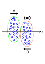
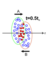
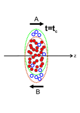
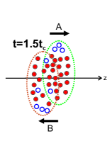
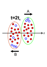
Figure 1: Schematic drawing of the system evolution in the proposed model. Blue points indicate nucleons which have not interacted before present time moment while red points indicate nucleons which already have interacted.

II.2 Partition into spectators and participants

In this section we describe the process of partition of nucleons into spectators and participants. We assume that nucleons coming from the target (projectile) become participants in collisions with nucleons from projectile (target). We define $f^{S}_{A(B)}(t,\mathbf{r},\mathbf{p})$ as the distribution function of nucleons from the target (projectile), which had not taken part in any reactions before time $t$ in the collider c.m. frame. It is seen from the definition that, at $t\to\infty$, this distribution function describes all spectators in the collision. Following this definition and also the above-mentioned assumption about collisions where nucleons become participants, we can describe the functions $f^{S}_{A(B)}(t,\mathbf{r},\mathbf{p})$ by the Boltzmann transport equation by assuming binary collisions, local molecular chaos, and collision integrals containing only “loss” terms. For instance, for nucleons from the target we have

$$p^{\mu}\partial_{\mu}f_{A}^{S}(t,\mathbf{r},\mathbf{p})=-\frac{1}{2}\int\frac{d^{3}p_{1}}{E_{p_{1}}}\,\frac{d^{3}p^{\prime}}{E_{p^{\prime}}}\frac{d^{3}p^{\prime}_{1}}{E_{p^{\prime}_{1}}}f_{A}^{S}(t,\mathbf{r},\mathbf{p})\,f_{B}^{(0)}(t,\mathbf{r},\mathbf{p}_{1})W(p,p_{1}|p^{\prime},p_{1}^{\prime}),$$ (11)

where $W(p,p_{1}|p^{\prime},p_{1}^{\prime})$ is the transition rate.

In order to perform integrations in Eq. (11) we will use the transition rate $W(p,p_{1}|p^{\prime},p_{1}^{\prime})=s\,\sigma(s,\theta)\,\delta^{4}(p+p_{1}-p^{\prime}-p_{1}^{\prime})$ for elastic binary collisions, where $s\equiv(p+p_{1})^{2}$ and $\sigma(s,\theta)$ is the differential cross section of nucleon-nucleon collision.

Since we are only considering “loss” terms, only the total nucleon-nucleon cross section will be relevant for the final result. After integrating (11) over outgoing particle momenta $p^{\prime}$ and $p^{\prime}_{1}$ we get

$$p^{\mu}\partial_{\mu}f_{A}^{S}(t,\mathbf{r},\mathbf{p})=-\frac{1}{2}\int\frac{d^{3}p_{1}}{E_{p_{1}}}d\Omega\sigma(s,\theta)\frac{1}{2}\sqrt{s(s-4m^{2})}f_{A}^{S}(t,\mathbf{r},\mathbf{p})\,f_{B}^{(0)}(t,\mathbf{r},\mathbf{p}_{1}).$$ (12)

Taking into account that $\displaystyle\frac{1}{2}\int d\Omega\sigma(s,\theta)=\sigma_{{}_{NN}}(s)$ and using explicit expression for $f_{A}^{(0)}$ (10) we perform the integration over $p_{1}$

$$p^{\mu}\partial_{\mu}f_{A}^{S}(t,\mathbf{r},\mathbf{p})=-\frac{\sigma_{{}_{NN}}(s)}{E_{p_{0}}}\frac{1}{2}\sqrt{s(s-4m^{2})}f_{A}^{S}(t,\mathbf{r},\mathbf{p})\,\rho_{B}^{(0)}(t,\mathbf{r}).$$ (13)

Since $f_{A}^{S}(t,\mathbf{r},\mathbf{p})$ describes nucleons, which did not take part in any reactions, it can be expressed as

$$f_{A}^{S}(t,\mathbf{r},\mathbf{p})=\rho_{A}^{S}(t,\mathbf{r})\,\delta^{2}(\mathbf{p}_{\perp})\,\delta(p_{z}-p_{A}),$$ (14)

where $p_{A}=-p_{B}=p_{0}$ and $\rho_{A}^{S}(t,\mathbf{r})$ is the time-dependent spatial density of the spectator nucleons. Then, taking into account that $E_{p_{0}}=\displaystyle\frac{\sqrt{s}}{2}$ and $p_{0}=\displaystyle\frac{1}{2}(s-4m^{2})^{1/2}$, we get the equation for $\rho_{A}^{S}(t,\mathbf{r})$

$$p_{0}^{\mu}\partial_{\mu}\rho_{A}^{S}(t,\mathbf{r}) = -2\sigma_{{}_{NN}}p_{0}\rho_{A}^{S}(t,\mathbf{r})\,\rho_{B}^{(0)}(t,\mathbf{r}),$$ (15)

$$\rho_{A}^{S}(t_{0},\mathbf{r}) = \rho_{A}^{(0)}(t_{0},\mathbf{r}).$$ (16)

Here the expression on the right-hand side of Eq. (15) is proportional to the number of binary collisions in the four-volume element at $(t,\mathbf{r})$, between any nucleons from target (B) and those nucleons from projectile (A), which had not yet interacted at time $t$. It is seen that this expression depends only on spatial densities, relative velocity and the nucleon-nucleon cross section. Thus, if we regard $\sigma_{{}_{NN}}$ as the total nucleon-nucleon cross section then Eq. (16) also describes the loss of the non-interacting nucleons due to any binary reactions of nucleons and not just due to elastic collisions. The solution of Eq. (15) with initial condition (16) can be written as

$$\rho_{A}^{S}(t,\mathbf{r})=\rho_{A}^{(0)}(t,\mathbf{r})\,\exp\left\{-2\sigma_{{}_{NN}}v_{0}\int_{t_{0}}^{t}dt^{\prime}\rho_{B}^{(0)}[t^{\prime},\mathbf{r}-\mathbf{v}_{A}(t-t^{\prime})]\right\},$$ (17)

where $v_{0}=p_{0}/E_{p_{0}}$ and $\mathbf{v}_{A}=(0,0,v_{0})$. Similarly, for nucleons from the projectile we have

$$\rho_{B}^{S}(t,\mathbf{r})=\rho_{B}^{(0)}(t,\mathbf{r})\,\exp\left\{-2\sigma_{{}_{NN}}v_{0}\int_{t_{0}}^{t}dt^{\prime}\rho_{A}^{(0)}[t^{\prime},\mathbf{r}-\mathbf{v}_{B}(t-t^{\prime})]\right\},$$ (18)

where $\mathbf{v}_{B}=(0,0,-v_{0})$.

II.3 Transverse distribution of spectators

It is easy to see similarities between our model and the optical limit of the Glauber-Sitenko approach GlauberSitenko applied for the description of relativistic heavy-ion collisions. Indeed, in our simplified kinetic approach we consider only binary collisions between nucleons which always move in the forward-backward direction, and the probability of binary interaction is determined by the total nucleon-nucleon cross section. One of the quantities which can be evaluated in that approach is the transverse distribution $T^{\rm part}(x,y)$ of the wounded nucleons (participants) BialasNWM ; GlauberModel , which is often used to define initial conditions in fluid dynamical models assuming that the transverse expansion of the interacting system is small during the initial pre-equilibrium phase. This distribution reads as

$$T^{\rm part}(x,y)=T_{A}^{\rm part}(x,y)+T_{B}^{\rm part}(x,y)$$

$$=T_{A}(x-b/2,y)\left[1-\left(1-\frac{\sigma_{{}_{NN}}T_{B}(x+b/2,y)}{A}\right)^{A}\right]$$

$$\quad+T_{B}(x+b/2,y)\left[1-\left(1-\frac{\sigma_{{}_{NN}}T_{A}(x-b/2,y)}{A}\right)^{A}\right]$$

$$\approx T_{A}(x-b/2,y)\,\left[1-\exp\left\{-\sigma_{{}_{NN}}T_{B}(x+b/2,y)\right\}\right]+$$

$$\quad T_{B}(x+b/2,y)\,\left[1-\exp\left\{-\sigma_{{}_{NN}}T_{A}(x-b/2,y)\right\}\right],$$ (19)

where $T_{A(B)}(x,y)=\int dz\,\rho_{{}_{WS}}(x,y,z)$ is the nuclear thickness function (normalized to $A$). Consequently, the transverse distribution of spectators can be written as

$$T^{\rm spec}(x,y)=T^{\rm tot}(x,y)-T^{\rm part}(x,y)$$

$$=T_{A}(x-b/2,y)\left(1-\frac{\sigma_{{}_{NN}}T_{B}(x+b/2,y)}{A}\right)^{A}+T_{B}(x+b/2,y)\left(1-\frac{\sigma_{{}_{NN}}T_{A}(x-b/2,y)}{A}\right)^{A}$$

$$\approx T_{A}(x{-}b/2,y)\,\exp\left\{-\sigma_{{}_{NN}}T_{B}(x{+}b/2,y)\right\}+T_{B}(x{+}b/2,y)\,\exp\left\{-\sigma_{{}_{NN}}T_{A}(x{-}b/2,y)\right\}.$$ (20)

To make a quantitative comparison of our model with the above-mentioned approach we calculate the transverse distribution of spectators within our model. To account for all possible nucleon interactions we let the initial time moment $t_{0}\to-\infty$. Then the transverse distribution of spectators from projectile $T_{A}^{\rm spec}(x,y)$ can be calculated as

$$T_{A}^{\rm spec}(x,y) = \lim_{t\to\infty}\int d\mathbf{p}\int dz\,f_{A}^{S}(t,\mathbf{r},\mathbf{p})$$ (21)

$$= \lim_{t\to\infty}\int dz\,\rho_{A}^{(0)}(t,\mathbf{r})\,\exp\left\{-2\sigma_{{}_{NN}}v_{0}\int_{-\infty}^{t}dt^{\prime}\rho_{B}^{(0)}[t^{\prime},\mathbf{r}-\mathbf{v}_{A}(t-t^{\prime})]\right\}.$$

To perform the integration in the exponent we use

$$\rho_{B}^{(0)}[t^{\prime},\mathbf{r}-\mathbf{v}_{A}\left(t-t^{\prime}\right)]=\gamma_{0}\,\rho_{{}_{WS}}[x+b/2,y,\gamma_{0}(z-v_{0}t+2v_{0}t^{\prime}-v_{0}t_{c})]\ ,$$

and make the transformation of the integration variable: $\displaystyle t^{\prime}=\frac{1}{2v_{0}\gamma_{0}}\left[z^{\prime}-\gamma_{0}z+v_{0}\gamma_{0}(t+t_{c})\right]$. By using that $t\to\infty$ and also the definition of the nuclear thickness function we can perform the integration over the new variable $z^{\prime}$ under the exponent and get

$$T_{A}^{\rm spec}(x,y)=\lim_{t\to\infty}\int dz\,\rho_{A}^{(0)}(t,\mathbf{r})\,\exp\left\{-\sigma_{0}T_{B}(x+b/2,y)\right\}.$$ (22)

By using that $\int dz\,\rho_{A}^{(0)}(t,\mathbf{r})=T_{A}(x-b/2,y)$ we finally get

$$T_{A}^{\rm spec}(x,y)=T_{A}(x-b/2,y)\,\exp\left\{-\sigma_{{}_{NN}}T_{B}(x+b/2,y)\right\}.$$ (23)

Similarly, the transverse distribution of spectators from projectile reads as

$$T_{B}^{\rm spec}(x,y)=T_{B}(x+b/2,y)\,\exp\left\{-\sigma_{{}_{NN}}T_{A}(x-b/2,y)\right\}.$$ (24)

Comparing Eqs. (23)-(24) with (20) we can conclude that our model is consistent with the Glauber-based approach for describing heavy-ion collisions. Furthermore, it provides the possibility of studying the time-dependent features of the spectator-participant partition process in the early stage of the nucleus-nucleus collision. Comparison of our model with MC-Glauber is presented in Appendix A.

III Calculation results

To study the temporal structure of the partition of spectators and participants we consider the time-dependent transverse distribution $T^{\rm s}(t;x,y)$ of the nucleons, which did not interact before time $t$. This distribution reads

$$T^{\rm s}(t;x,y) = T_{A}^{\rm s}(t;x,y)+T_{B}^{\rm s}(t;x,y),$$ (25)

$$T_{A(B)}^{\rm s}(t;x,y) = \int d\mathbf{p}\int dz\,f_{A(B)}^{S}(t,\mathbf{r},\mathbf{p})$$ (26)

$$= \int dz\,\rho_{A(B)}^{(0)}(t,\mathbf{r})\,\exp\left\{-2\sigma_{{}_{NN}}v_{0}\int_{-\infty}^{t}dt^{\prime}\rho_{B(A)}^{(0)}[t^{\prime},\mathbf{r}-\mathbf{v}_{A(B)}(t-t^{\prime})]\right\}.$$

We can rewrite this expression in terms of the initial Woods-Saxon distribution:

$$T_{A(B)}^{\rm s}(t;x,y) = \int dz\,\gamma_{0}\rho_{{}_{WS}}(x\mp b/2,y,\gamma_{0}[z\mp v_{0}(t-t_{c})])\times$$ (27)

$$\quad\exp\left\{-2\sigma_{{}_{NN}}v_{0}\int_{t_{0}}^{t}dt^{\prime}\gamma_{0}\rho_{{}_{WS}}(x\pm b/2,y,\gamma_{0}[z\mp v_{0}(t{+}t_{c})\pm 2v_{0}t^{\prime}])\right\}\ .$$

It is useful to introduce the variables $\tilde{z}=\gamma_{0}z$ and $\tilde{t}=t/t_{c}$, where, as previously defined, $t_{c}=R_{0}/(\gamma_{0}v_{0})$, is the time of the maximum overlap of the colliding nuclei (see Fig. 1). Studies within Monte Carlo cascade models have shown that this time moment corresponds to the maximum of the nucleon-nucleon collision frequency Anchishkin2010 ; Anchishkin2013PRC ; Anchishkin2013 and it appears to be a natural energy-dependent temporal scale for the initial stage of the collision. This time, $t_{c}$, decreases with increasing collision energy and lies in the range: $t_{c}\simeq 1$ to $2$ fm/$c$ at energies of the CERN Super Proton Synchrotron (SPS), $t_{c}\simeq 0.1$ to $0.8$ fm/$c$ at energies of the BNL Relativistic Heavy Ion Collider (RHIC) and $t_{c}\sim 10^{-2}$ to $10^{-3}$ fm/$c$ at energies of the Large Hadron Collider (LHC). Equation (27) is then rewritten as

$$T_{A(B)}^{\rm s}(\tilde{t};x,y) = \int d\tilde{z}\rho_{{}_{WS}}[x\mp b/2,y,\tilde{z}\mp R_{0}(\tilde{t}-1)]\times$$ (28)

$$\quad\exp\left\{-2\sigma_{{}_{NN}}R_{0}\int_{-\infty}^{\tilde{t}}d\tilde{t}^{\prime}\rho_{{}_{WS}}[x\pm b/2,y,\tilde{z}\mp R_{0}(\tilde{t}+1)\pm 2R_{0}\tilde{t}^{\prime}]\right\}.$$

III.1 Number of participants

The total number of participants (net-baryon participant number) at time $t$ can be obtained as

$$N_{\rm part}(t)=2A-\int dxdy\left[T_{A}^{\rm s}(t;x,y)+T_{B}^{\rm s}(t;x,y)\right].$$ (29)

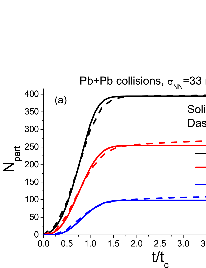
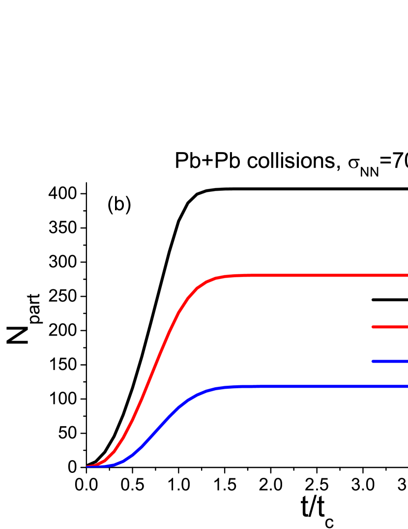
Figure 2: The time dependence of the total number of participant nucleons in Pb+Pb collisions at (a) SPS and RHIC energies ($\sigma_{{}_{\rm NN}}=33$ mb) and (b) LHC energy ($\sigma_{{}_{\rm NN}}=70$ mb) for different values of impact parameter. Solid lines depict calculations in the proposed model while dashed lines in panel (a) correspond to calculations from the UrQMD model at $\sqrt{s_{{}_{\rm NN}}}=17.3$ GeV.

The time dependence of the total number of participant nucleons in Pb-Pb collisions is depicted in Fig. 2 for (a) SPS and RHIC energies ($\sigma_{{}_{\rm NN}}=33$ mb) and (b) LHC energy ($\sigma_{{}_{\rm NN}}=70$ mb) at three different centralities: $b=0,0.4b_{\rm max},0.7b_{\rm max}$, where $b_{\rm max}=2R_{0}$ and $R_{0}=6.53$ fm. We can see that a change in the nucleon-nucleon cross section, which roughly corresponds to the increase of the collision energy from RHIC to LHC, has little influence on the time dependence of $N_{\rm part}(t)$ and only slightly increases the total number of participant nucleon charge at the given impact parameter. It is seen from Fig. 2 that the formation of the participant system is the most intense in the time range $t\simeq 0.5t_{c}$ to $1t_{c}$ and becomes complete at about $t=1.5t_{c}$.

It makes sense to make a comparison of predictions regarding time dependence of our simplified analytic model with a more complicated cascade model such as the ultrarelativistic quantum molecular dynamics (UrQMD) transport approach UrQMD1998 ; UrQMD1999 . The time dependence of the average total number of participant net nucleons (baryons) can be calculated in UrQMD as event-by-event average of $N_{\rm part}(t)=2A-N_{\rm spec}(t)$, where $N_{\rm spec}(t)$ is determined in each event by analyzing the collision history. UrQMD results for $N_{\rm part}(t)$ in Pb+Pb collisions at top SPS energy of $\sqrt{s_{{}_{\rm NN}}}=17.3$ GeV are depicted by dashed lines in Fig. 2a. We note that the temporal axis in UrQMD is specially aligned in Fig. 2a with the one used in our model so that the time moment $t=0$ correspond to two colliding nuclei “touching” each other. The comparison of UrQMD with calculations of our model (solid lines in Fig. 2) shows generally good agreement between our model and UrQMD. One can see, however, that the number of participants in UrQMD keeps increasing, albeit insignificantly, also at times $t>1.5t_{c}$, which can be attributed to the more complex collision dynamics of UrQMD compared to our analytic model.

III.2 Angular momentum

Another important quantity, of which the time dependence can be studied within the proposed model, is the total angular momentum of the participant system. The total angular momentum of the formed participant system is non-zero in non-central collisions Becattini2008 ; Gao2008 and can attain a significantly large value ($L\approx 10^{6}\hbar$ for LHC energies Vovchenko2013 ). The angular momentum illustrates the initial rotation of the system of participants, and it was shown that it depends strongly on the initial nuclear density profile and leaves some freedom for the assumed initial state of the participant system in fluid dynamical and in molecular dynamics models. The time-dependent total angular momentum, $L_{\rm tot}^{P}(t)$, of the participant system can be calculated in our model as the difference of total angular momentum, $L_{\rm tot}$, and the time-dependent angular momentum, $L_{\rm tot}^{S}(t)$, of nucleons, which did not interact before time $t$. These quantities can be written as

$$L_{\rm tot} = p^{z}_{\rm in}\int dxdy\,x\left[T_{A}(x-b/2,y)-T_{B}(x+b/2,y)\right],$$ (30)

$$L_{\rm tot}^{S}(t) = p^{z}_{\rm in}\int dxdy\,x\left[T_{A}^{S}(t;x,y)-T_{B}^{S}(t;x,y)\right],$$ (31)

$$L_{\rm tot}^{P}(t) = L_{\rm tot}-L_{\rm tot}^{S}(t),$$ (32)

where $p^{z}_{\rm in}=(s/4-m_{N}^{2})^{1/2}$ is the initial momentum of a nucleon.

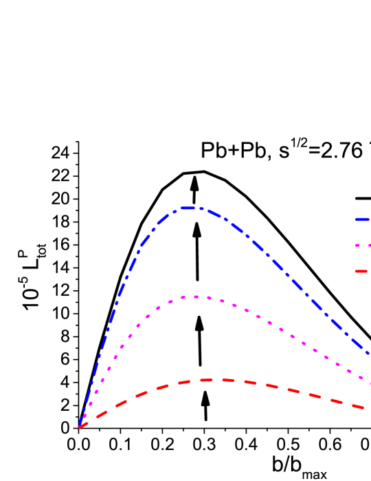
Figure 3: The dependence of the total angular momentum of the participant system on impact parameter at different times for Pb+Pb collisions at $\sqrt{s}=2.76$ TeV.

The dependence of the total angular momentum of the participant system on impact parameter at different times is depicted in Fig. 3. The values of the angular momentum are in units of $\hbar$. It can be seen that, similarly to the case of the total number of participants, the total angular momentum of the participant system increases with time and reaches its maximum value for each particular collision centrality at the end of the spectator-participant partition process.

It is also interesting to consider the time evolution of the angular momentum of participants per participant (per baryon charge of participants). We note that the number of participants also changes with time. Such a quantity contains information about an average contribution of participant nucleons to the total angular momentum. The dependence of this quantity on impact parameter at different times is depicted in Fig. 4. It can be seen that, similarly to the total angular momentum of participants, the angular momentum per participant increases with time for any value of the impact parameter. This means that, for any fixed value of impact parameter $b$, the rate of increase of the total number of participants, $N_{p}$, is smaller than the rate of increase of the total angular momentum of participants. Another similarity is that there is also maximum in the dependence of this quantity on impact parameter which is shifted in the direction of a larger $b$. One difference is that the angular momentum per participant is non-vanishing for large $b$, indicating that the initial rotation and local vorticity are significant in the range of semi-central to even the most peripheral collisions and needs to be accounted for.

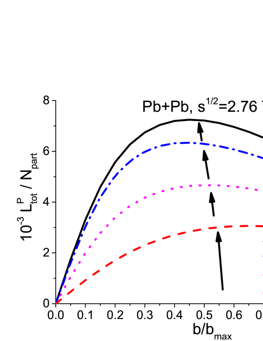
Figure 4: The dependence of the participant angular momentum per participant on impact parameter at different times for Pb+Pb collisions at $\sqrt{s}=2.76$ TeV.

It can be interesting to compare the rate of the increase with time of the angular momentum of participants with a similar rate concerning the total number of participant nucleons. In order to do that, we compare the time dependencies of the normalized quantities $N_{\rm part}(t)/N_{\rm part}(\infty)$ and $L_{\rm tot}^{P}(t)/L_{\rm tot}^{P}(\infty)$, where $N_{\rm part}(\infty)$ and $L_{\rm tot}^{P}(\infty)$ are the values of the total number of participants and of the total angular momentum of participants at the end of the spectator-participant separation stage. The time dependence of the above-mentioned quantities is depicted in Fig. 5.

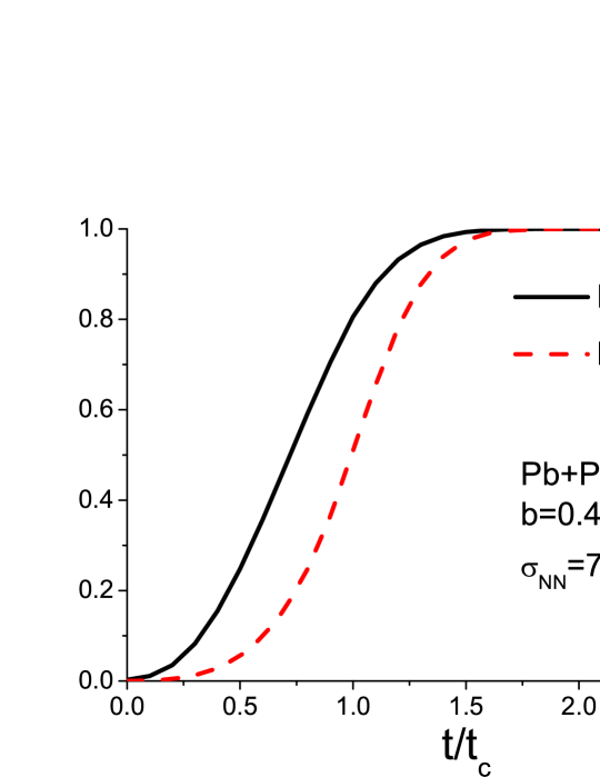
Figure 5: The time dependence of the total number of participant nucleons and of the total angular momentum of participants divided by their final values in Pb+Pb collisions.

It can be seen from Fig. 5 that the process of increase of the angular momentum of participants happens at a somewhat later time in comparison to the total number of participants, and the most significant increase happens in time interval $t\simeq 0.75t_{c}$ to $1.25t_{c}$. The reason for this is that different nucleons carry different contributions to the total participant angular momentum, and most of the nucleons with the largest contribution become participants at later times, which is also evident from the time dependence of the angular momentum of participants related to the number of participants (see Fig. 4).

III.3 Vorticity

The classical (non-relativistic) vorticity of the participants in the reaction plane, $(x,z)$, is defined as

$$\omega_{y}=\omega_{xz}=-\omega_{zx}=\frac{1}{2}\left(\partial_{z}v_{x}^{P}-\partial_{x}v_{z}^{P}\right),$$ (33)

where $\mathbf{v}^{P}$ is the average 3-velocity of participants. The emergence of the vorticity in the reaction plane in heavy-ion collisions is attributed to initial angular momentum of the participant system and studies within fluid dynamical models had shown that vorticity still remains significant during the freeze-out stage Csernai2013 . Along with angular momentum such a quantity can be used to study rotation in the reaction plane. Another closely related quantity is $\Lambda$ polarization which can be detectable experimentally Becattini2013 . The possibility to detect rotation via differential Hanbury Brown and Twiss (HBT) has also recently been explored CsernaiHBT1 ; CsernaiHBT2 .

While in our simplified model we do not consider the subsequent evolution of the formed participant system, most importantly the equilibration process, we can still study the emergence of the vorticity during the formation of this system. To do this we assume that the transverse motion of participants is small during the formation stage (“no-stopping” mode) and their average velocity can be expressed as

$$v_{x}^{P}(t,\mathbf{r})\approx v_{y}^{P}(t,\mathbf{r}) \approx 0,$$ (34)

$$v_{z}^{P}(t,\mathbf{r}) \approx v_{0}\,\frac{\rho_{A}^{P}(t,\mathbf{r})-\rho_{B}^{P}(t,\mathbf{r})}{\rho_{A}^{P}(t,\mathbf{r})+\rho_{B}^{P}(t,\mathbf{r})},$$ (35)

$$\rho_{A(B)}^{P}(t,\mathbf{r}) \approx \rho_{A(B)}^{(0)}(t,\mathbf{r})-\rho_{A(B)}^{S}(t,\mathbf{r}).$$ (36)

Here $\rho_{A(B)}^{P}(t,x,y,z)$ is the time-dependent spatial density of participant nucleons from the target (projectile). For the relativistic case we follow the definition from Ref. Molnar2010

$$\omega_{\nu}^{\mu}=\frac{1}{2}\left(\nabla_{\nu}u^{\mu}-\nabla^{\mu}u_{\nu}\right),$$ (37)

where $u^{\mu}=\gamma(1,\mathbf{v})$, $\nabla_{\alpha}=\Delta_{\alpha}^{\beta}\partial_{\beta}$ and $\Delta^{\mu\nu}=g^{\mu\nu}-u^{\mu}u^{\nu}$. Similarly to Ref. Csernai2013 we neglect the collective acceleration in comparison with rotation, i.e., $|\partial_{\tau}u^{\mu}|\ll|\partial_{x}u^{z}|$, and get the following expression for the relativistic vorticity $\omega_{z}^{x}$ in the reaction plane

$$\omega_{z}^{x}=-\omega_{x}^{z}=-\frac{1}{2}\gamma\partial_{x}v_{z}-\frac{1}{2}v_{z}\partial_{x}\gamma,$$ (38)

where $\gamma=(1-v_{z}^{2})^{-1/2}$. Here we already take into account that $v_{x}=v_{y}=0$ in our model.

Similarly to Ref. Csernai2013 , we also use the weights proportional to the energy density to better reflect the collective dynamics. The energy-density weighted vorticity for both classical and relativistic cases is then

$$\Omega_{zx}=w(t,x,z)\omega_{zx},$$ (39)

where the weight, $w(t,x,z)$, is

$$w(t,x,z)=\frac{\epsilon^{P}(t,x,y=0,z)}{\langle\epsilon^{P}(t,x,y=0,z)\rangle}.$$ (40)

Here, $\epsilon^{P}(t,x,y,z)=\displaystyle\frac{\sqrt{s}}{2}\left(\rho_{A}^{P}+\rho_{B}^{P}\right)$ is the energy density of the participants and $\langle\epsilon^{P}(t,x,y=0,z)\rangle$ is the average energy density in the reaction plane at time $t$. For averaging we use the region $-1.5R_{0}<x<1.5R_{0},\,-1.5R_{0}<\gamma_{0}z<1.5R_{0}$. Results of the calculations of the classical and relativistic weighted vorticity in the reaction plane at different time moments are presented in Figs. 6-8.

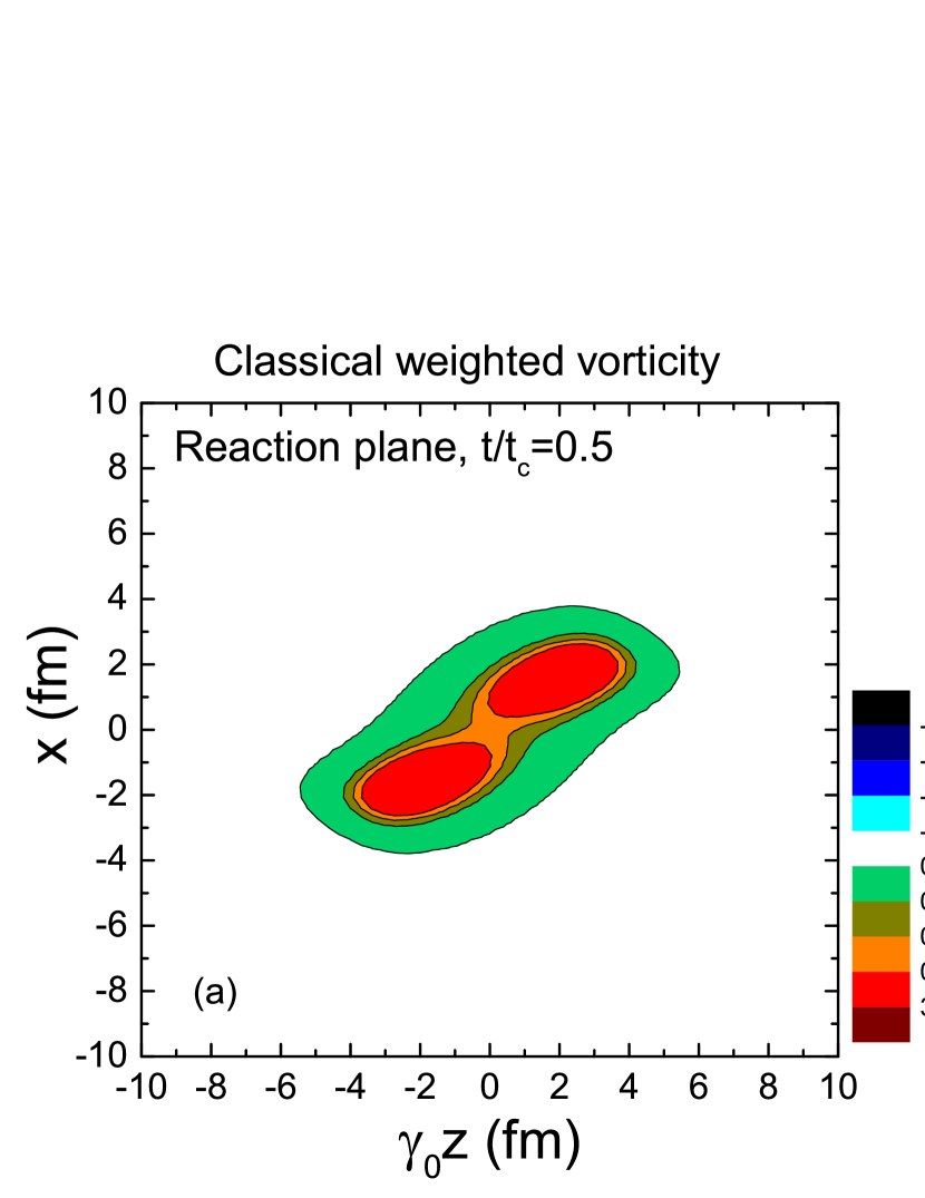
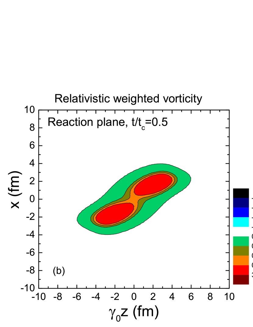
Figure 6: The (a) classical and (b) relativistic weighted participant vorticity, $\Omega_{zx}$, in units of $c$/fm, calculated in the reaction plane, i.e. $(xz)$ plane, at time moment $t=0.5t_{c}$ in Pb+Pb collisions. The collision energy is $\sqrt{s_{{}_{NN}}}=2.76$ TeV and $b=0.7b_{\rm max}$. The collision axis $z$ is scaled with $\gamma$-factor $\gamma_{0}$, which corresponds to the collision energy.

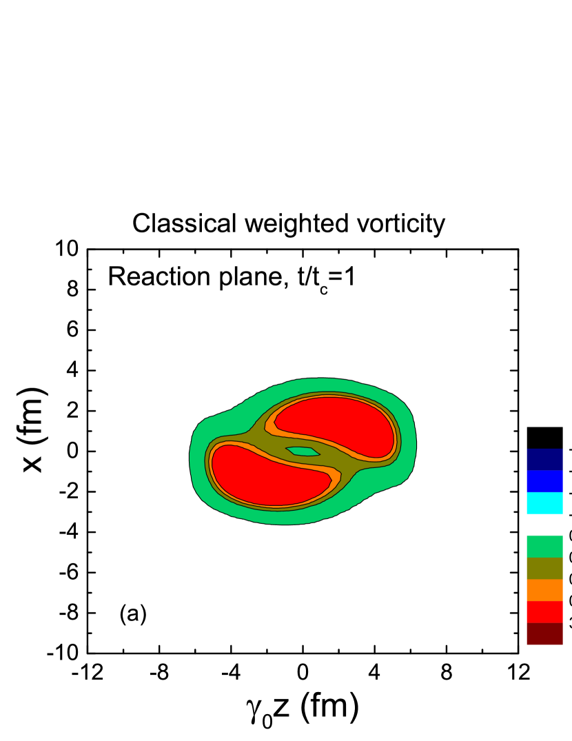
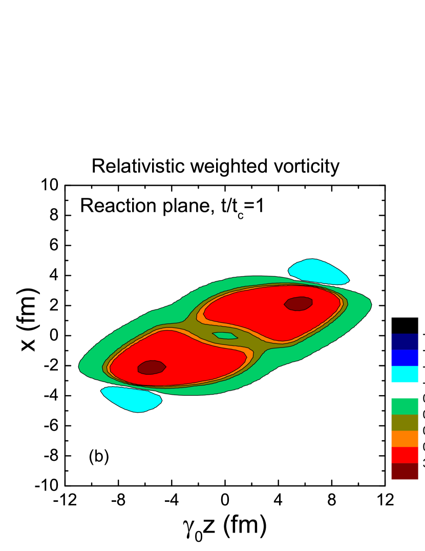
Figure 7: Same as Fig. 6, but for $t=t_{c}$.

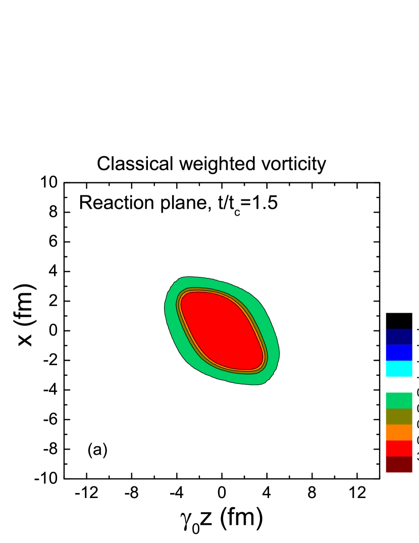
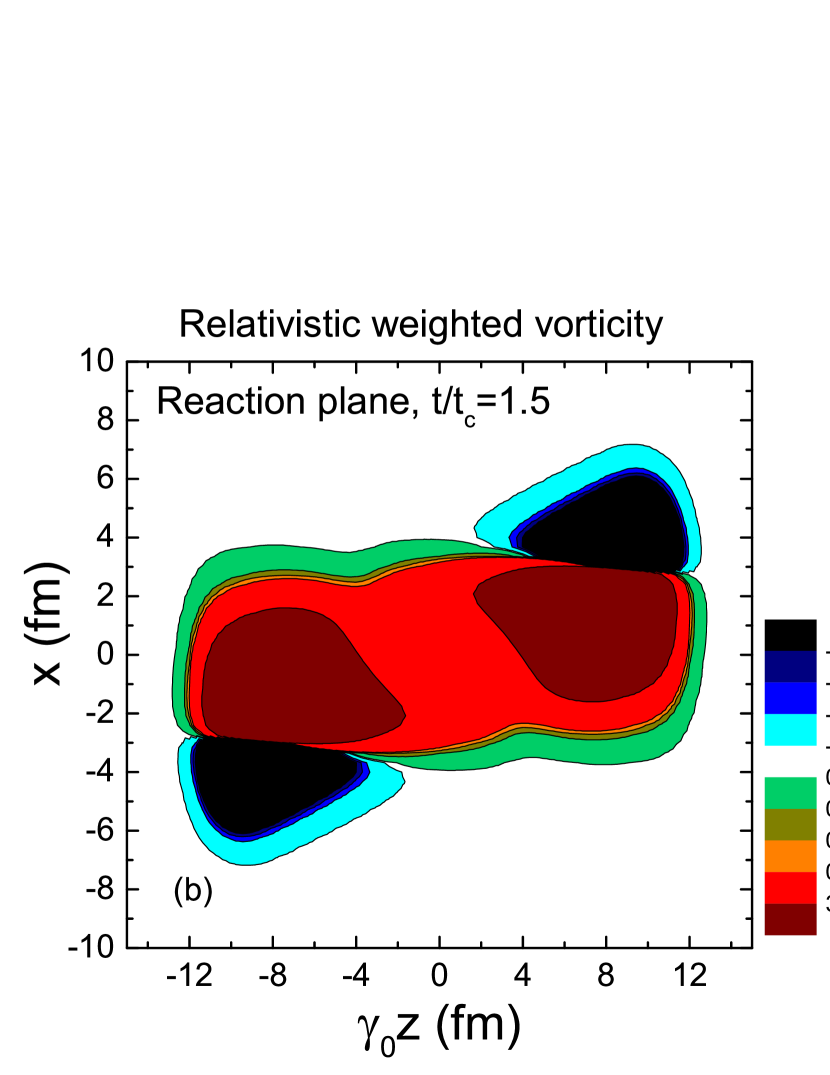
Figure 8: Same as Fig. 6, but for $t=1.5t_{c}$.

The presented results illustrate the emergence of rotation during the formation of the participant system. Also, it is seen that there may exist substantial differences in results when using different definitions of vorticity indicating that its relativistic generalization is not trivial. It should also be noted, however, that the proposed model does not describe the evolution of the participant system after its formation and using the “no-stopping” assumption, Eq. (36), allows us to only give qualitative rather than quantitative picture, especially for times $t>t_{c}$.

IV Conclusions

The identification of different stages of the initial state is important if we want to discuss the results of multimodule models or hybrid models. While the middle part of a heavy ion reaction is usually well described by the fluid dynamical model, different initial states and different final-state approximations are used in such kinds of combined models.

In the Particle in Cell relativistic (PICR) fluid dynamical model hydro1 ; hydro2 the initial state assumes a dynamical evolution in a Yang-Mills field theoretical model M1 ; M2 , which has some features similar to the model presented here. The time when the PICR calculation starts corresponds to a configuration when the two nuclei have interpenetrated each other and were near to be stopped by the Yang-Mills field. In the timescale of this model this configuration corresponds to a time moment not earlier than $2t_{c}$. The subsequent (3+1)-dimensional fluid dynamical development led to increased rotation due to the Kelvin-Helmholtz Instability (KHI) in certain favorable configurations. The initial time moment of the hydrodynamical evolution in the hybrid approach based on UrQMD model Petersen2008 is also closely related to the temporal scale $t_{c}$ of our model. There $2t_{c}$ is assumed to be the earliest possible thermalization time and, consequently, the earliest possible initial time moment of the hydrodynamical evolution, which should not be smaller than 1 fm/$c$.

The present model is based on a conserved nucleon picture. For example, the angular momentum per nucleon assumes conserved nucleons. At very high energies numerous hadron pairs are created including baryon pairs, so the concept of the model should be implemented for the conserved baryon charge.

Physically, the prehydrodynamical stage will remain nearly the same; however, the high parton density may influence the dynamics already after $t_{c}$. Especially, collective force fields may change the dynamics, and may speed up equilibration, which then leads to collective effects like the KHI.

The vorticity characteristics shown in Fig. 8 are interesting. The participant domain has substantial positive vorticity. This agrees well with the fluid dynamical calculations. The spectators show negative vorticity, this is arising from the particle loss due to collisions from the spectator domain. Because the spectators are not considered at all in the PICR calculations this effect is not covered by these model calculations.

Notice the large difference between the non-relativistic and relativistic vorticities in Figs. 7 and 8. This is due to the relativistic $\gamma$ factors, which are large in the present calculation as there are only collisions, no collective forces or pressure. In the PICR calculations these collective interactions decrease velocity differences both in the initial state model and in the fluid dynamics, thus the difference between the non-relativistic and relativistic vorticities is modest.

The initial state model in the PICR calculations is dominated by attractive collective Yang-Mills fields, which keep the system more compact and uniform. Some versions of the Color-glass Condensate (CGC) initial state models have similar features. Also in the PICR model sharp initial nuclear surfaces are assumed instead of Woods-Saxon surface profiles. This makes the typical times $t_{c}$ and $2t_{c}$ shorter. On the other hand for molecular dynamics models (or to some extent for hybrid models) with MC-Glauber initialization the present model provides a good estimate for the initial times. See Appendix A.

The formation of a quark-gluon plasma (QGP) leads to more rapid equilibration and to critical fluctuations. These also facilitate the equilibration of rotation especially in low viscosity fluid dynamical models like PICR with KHI. Before the final hadronization the perturbative vacuum may keep the participant system more compact and then rapid hadronization from a supercooled QGP has the best chances to show observable signs of rotation at the final freeze out. To detect the observable signs of Global Collective Flow patterns these should be separated from random fluctuations as described in Ref. CS14 .

At the same time, for the development of the initial rotation and vorticity the present model provides an excellent guidance for all dynamical models of peripheral heavy ion reactions.

Appendix

IV.1 Reaction density of binary collisions

Our model gives the possibility to calculate the density, $\Gamma(t,\mathbf{r})$, of binary collisions between nucleons from colliding nuclei, which describes the number of binary reactions per unit volume per unit time. Since these binary collisions are beam directed, the relative velocity of nucleons is $2v_{0}$. Exploiting this and taking into account the ballistic distribution functions $f^{(0)}_{A(B)}$ of the colliding nucleons [see Eq. (10)] one can write down the four-density of binary reactions as

$$\Gamma_{\rm coll}(t,\mathbf{r})=\sigma_{{}_{NN}}\,2v_{0}\,\rho_{A}^{(0)}(t,\mathbf{r})\,\rho_{B}^{(0)}(t,\mathbf{r}).$$ (41)

The total average number of binary collisions $N_{\rm coll}$ is

$$N_{\rm coll} = \int dt\,d\mathbf{r}\,\Gamma_{\rm coll}(t,\mathbf{r})$$

$$=\sigma_{{}_{NN}}\,2v_{0}\gamma_{0}^{2}\int dt\,d\mathbf{r}\,\rho_{{}_{WS}}\big{(}x-b/2,y,\gamma_{0}[z-v_{0}(t-t_{c})]\big{)}\,\rho_{{}_{WS}}\big{(}x+b/2,y,\gamma_{0}[z+v_{0}(t-t_{c})]\big{)}\,.$$

Making a change of variables $(t,z)\to(z_{1},z_{2})$ as $z_{1}=\gamma_{0}[z-v_{0}(t-t_{c})]$, $z_{2}=\gamma_{0}[z+v_{0}(t-t_{c})]$ we get

$$N_{\rm coll} = \sigma_{{}_{NN}}\int d\mathbf{r}_{\perp}\int dz_{1}\,\rho_{{}_{WS}}\big{(}x-b/2,y,z_{1}\big{)}\int dz_{2}\,\rho_{{}_{WS}}\big{(}x+b/2,y,z_{2}\big{)}$$ (43)

$$= \sigma_{{}_{NN}}\int dxdy\,T_{A}\big{(}x-b/2,y\big{)}\,T_{B}\big{(}x+b/2,y\big{)}\,=\,\sigma_{{}_{NN}}A^{2}\,t(b),$$

where $t(b)$ is the nuclear overlap function, normalized to unity, which depends on the impact parameter. Equation (43) coincides with the expression for average number of binary collisions in the analytical Glauber model. Our model, however, allows one to study also the temporal and longitudinal structure of the binary collisions.

Let us consider the quantity $\tilde{\Gamma}_{\rm coll}(t,z)=\int dxdy\Gamma_{\rm coll}(t,\mathbf{r})$, which represents the two-dimensional space-time structure of the binary collisions. This quantity is depicted in Fig. 9. It is instructive to compare the structure of two-dimensional binary collisions given in Fig. 9 with space-time reaction zones which were investigated in Ref. Anchishkin2013 exploiting UrQMD: very similar features of the distribution of collisions can be immediately found at earlier times. Besides, it is explicitly seen in Fig. 9 how natural and useful for the description of the initial stage is the time scale $t_{c}$, which is a unit of a measuring the time axis.

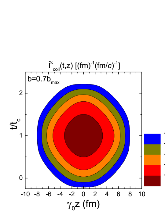
Figure 9: The binary reaction density $\tilde{\Gamma}_{\rm coll}(t,z)$ in coordinates $(t,z)$ in Pb+Pb collisions. The collision energy is $\sqrt{s_{{}_{NN}}}=2.76$ TeV and $b=0.7b_{\rm max}$. The collision axis, $z$, is scaled with $\gamma$-factor, $\gamma_{0}$, which corresponds to the collision energy.

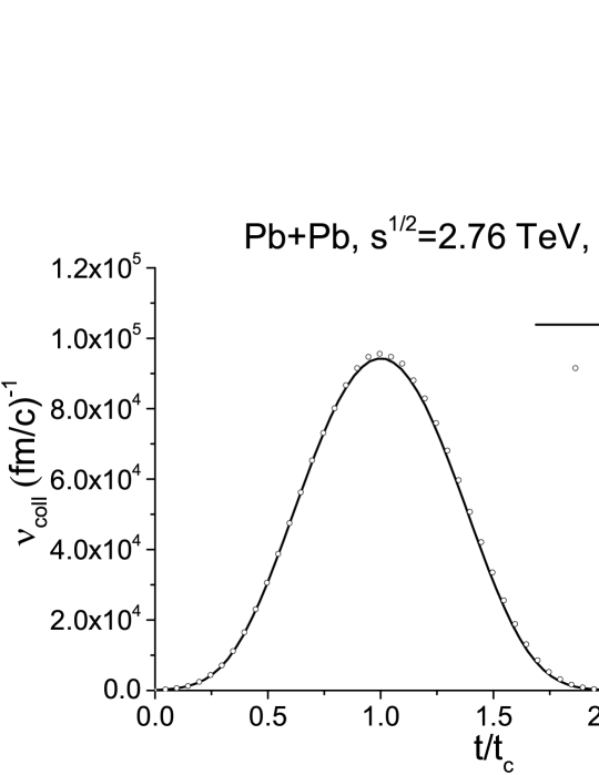
Figure 10: The frequency of binary collisions $\nu_{\rm coll}(t)$ in Pb+Pb collisions calculated in our model and in Glauber Monte Carlo. The collision energy is $\sqrt{s_{{}_{NN}}}=2.76$ TeV and $b=0.7b_{\rm max}$.

It is useful to make a comparison of our model to MC-Glauber. In MC-Glauber one can take into account correlations generated by the collision mechanism (dubbed “twin” correlations in Ref. Blaizot2014 ), i.e. that nucleons can only collide if they are close by in the transverse plane. In order to make a comparison we consider the frequency of binary reactions, $\nu_{\rm coll}(t)=\int dz\tilde{\Gamma}_{\rm coll}(t,z)$, which can be calculated in our model and also in MC-Glauber. To calculate this quantity in MC-Glauber we follow the usual procedure, recently described in Ref. ALICECentrality2013 , but also add additional step to determine time dependence:

1. We generate the initial positions of nucleons in colliding nuclei by using the Woods-Saxon distribution with the same parameters that are used in our analytical model.

2. We consider all possible binary collisions between the nucleons from different colliding nuclei by calculating the distance, $d_{\rm trans}$, between them in the transverse plane. In case it satisfies the inequality $\displaystyle d_{\rm trans}<\sqrt{\frac{\sigma_{{}_{NN}}}{\pi}}$, we register a binary collision.

3. We calculate the time moment for each binary collision as $\displaystyle t=\frac{|z_{1}-z_{2}|}{2v_{0}}$, where $z_{1}$ and $z_{2}$ are the longitudinal coordinates of the two colliding nucleons in the collider center-of-mass frame at $t=0$.

The frequency of binary reactions calculated in our analytical model and in the MC-Glauber are depicted in Fig. 10. It is seen that both graphs virtually coincide, which further indicates that our model is consistent with Glauber approach and also that event-by-event fluctuations and “twin” correlations have negligible effect on a frequency of the binary reactions.

References

- (1) R.J. Glauber, in Lectures in Theoretical Physics, edited by W.E. Britten and L.G. Dunham, Vol. 1 (Interscience, New York, 1959); A.G. Sitenko, Ukr. Fiz. Zh. 4, 152 (1959).
- (2) A. Bialas, M. Bleszynski, and W. Czyz, Nucl. Phys. B 111, 461 (1976).
- (3) M.L. Miller, K. Reygers, S.J. Sanders, and P. Steinberg, Annu. Rev. Nucl. Part. Sci. 57, 205 (2007).
- (4) P.F. Kolb, U.W. Heinz, P. Huovinen, K.J. Eskola, K. Tuominen, Nucl. Phys. A 696, 197 (2001).
- (5) P.F. Kolb, P. Huovinen, U. Heinz, H. Heiselberg, Phys. Lett. B 500, 232 (2001).
- (6) H. Holopainen, H. Niemi, and K.J. Eskola, Phys. Rev. C 83, 034901 (2011).
- (7) B. Schenke, S. Jeon, and C. Gale, Phys. Rev. Lett. 106, 042301 (2011).
- (8) Z. Qiu and U. Heinz, Phys. Rev. C 84, 024911 (2011).
- (9) W. Broniowski, P. Bożek, and M. Rybczyński, Phys. Rev. C 76, 054905 (2007).
- (10) B. Alver and G. Roland, Phys. Rev. C 81, 054905 (2010).
- (11) E. Retinskaya, M. Luzum, and J.-Y. Ollitrault, Phys. Rev. C 89, 014902 (2014).
- (12) T. Renk and H. Niemi, Phys. Rev. C 89, 064907 (2014).
- (13) J.I. Kapusta, Phys. Rev. C 81, 055201 (2010)
- (14) J.I. Kapusta, B. Müller, and M. Stephanov, Phys. Rev. C 85, 054906 (2012).
- (15) J.I. Kapusta, B. Müller, and M. Stephanov, Nucl. Phys. A 904-905, 499C (2013).
- (16) D. Anchishkin, A. Muskeyev, and S. Yezhov, Phys. Rev. C 81, 031902 (2010).
- (17) D. Anchishkin, V. Vovchenko, and L.P. Csernai, Phys. Rev. C 87, 014906 (2013).
- (18) D. Anchishkin, V. Vovchenko, and S. Yezhov, Int. J. Mod. Phys. E 22, 1350042 (2013).
- (19) S.A. Bass et al., Prog. Part. Nucl. Phys. 41, 255 (1998).
- (20) M. Bleicher et al., J. Phys. G 25, 1859 (1999).
- (21) F. Becattini, F. Piccinini, and J. Rizzo, Phys. Rev. C 77, 024906 (2008).
- (22) J.H. Gao, S.W. Chen, W.T. Deng, Z.T. Liang, Q. Wang, and X.N. Wang, Phys. Rev. C 77, 044902 (2008).
- (23) V. Vovchenko, D. Anchishkin, and L.P. Csernai, Phys. Rev. C 88, 014901 (2013).
- (24) L.P. Csernai, V.K. Magas, and D.J. Wang, Phys. Rev. C 87, 034906 (2013); L.P. Csernai, D.J. Wang, M. Bleicher, and H. Stöcker, Phys. Rev. C 90, 021904 (2014).
- (25) F. Becattini, L.P. Csernai, and D.J. Wang, Phys. Rev. C 88, 034905 (2013).
- (26) L.P. Csernai and S. Velle, arXiv:1305.0385 [nucl-th]; L.P. Csernai and S. Velle, Int. J. Mod. Phys. E 23, 1450043 (2014).
- (27) L.P. Csernai, S. Velle, and D.J. Wang, Phys. Rev. C 89, 034916 (2014).
- (28) E. Molnar, H. Niemi, and D.H. Rischke, Eur. Phys. J. C 65, 615 (2010).
- (29) L.P. Csernai, V.K. Magas, H. Stöcker, and D.D. Strottman, Phys. Rev. C 84, 024914 (2011).
- (30) L.P. Csernai, D.D. Strottman and Cs. Anderlik, Phys. Rev. C 85, 054901 (2012).
- (31) V.K. Magas, L.P. Csernai, and D.D. Strottman, Phys. Rev. C 64, 014901 (2001).
- (32) V.K. Magas, L.P. Csernai, and D.D. Strottman, Nucl. Phys. A 712, 167 (2002).
- (33) H. Petersen, J. Steinheimer, G. Burau, M. Bleicher, and H. Stöcker, Phys. Rev. C 78, 044901 (2008).
- (34) L.P. Csernai, and H. Stöcker, J. Phys. G in print, arXiv:1406.1153 [nucl-th].
- (35) J.-P. Blaizot, W. Broniowski, and J.-Y. Ollitrault, Phys. Rev. C 90, 034906 (2014).
- (36) B. Abelev et al. (ALICE Collaboration), Phys. Rev. C 88, 044909 (2013).