Dimensions of slowly escaping sets and annular itineraries for exponential functions

Abstract.

We study the iteration of functions in the exponential family. We construct a number of sets, consisting of points which escape to infinity ‘slowly’, and which have Hausdorff dimension equal to $1$. We prove these results by using the idea of an annular itinerary. In the case of a general transcendental entire function we show that one of these sets, the uniformly slowly escaping set, has strong dynamical properties and we give a necessary and sufficient condition for this set to be non-empty.

1. Introduction

This paper is principally concerned with transcendental entire functions in the exponential family, defined by

$$E_{\lambda}(z)=\lambda e^{z},\quad\text{for }\lambda\in\mathbb{C}\backslash\{0\}.$$

For a general transcendental entire function $f$, the Fatou set $F(f)$ is defined as the set $z~{}\in~{}\mathbb{C}$ such that $\{f^{n}\}_{n\in\mathbb{N}}$ is a normal family in a neighbourhood of $z$. The Julia set $J(f)$ is the complement in $\mathbb{C}$ of $F(f)$. An introduction to the properties of these sets was given in [1]. The escaping set, which was first studied for a general transcendental entire function in [10], is defined by

$$I(f)=\{z:f^{n}(z)\rightarrow\infty\text{ as }n\rightarrow\infty\}.$$

Many authors have studied the Hausdorff dimension of $I(E_{\lambda})$, or subsets of this set. We refer to [13] for a definition of Hausdorff dimension, which we denote here by $\dim_{H}$. A key result is that of McMullen [17], who showed that $\dim_{H}J(E_{\lambda})=2$. It is well-known that it follows from his construction that $\dim_{H}I(E_{\lambda})=2$.

When $\lambda\in(0,e^{-1})$ it is known – see [8, 9] – that $J(E_{\lambda})$ consists of an uncountable set of unbounded curves known as a Cantor bouquet, and that each curve, except possibly for its finite endpoint, lies in $I(E_{\lambda})$. In two celebrated papers [14, 15] Karpińska proved the paradoxical fact that the set consisting of these curves excluding their finite endpoints has Hausdorff dimension $1$, whereas the set of finite endpoints has Hausdorff dimension $2$. A somewhat related result is that of Karpińska and Urbański [16] who defined subsets of $I(E_{\lambda})$ of Hausdorff dimension $d$, for each $d\in(1,2)$.

In fact, all these papers considered a subset $A(E_{\lambda})$ of $I(E_{\lambda})$ known as the fast escaping set. The fast escaping set was introduced in [3], and can be defined [22] for a general transcendental entire function $f$ by

(1.1) $$A(f)=\{z:\text{there exists }\ell\in\mathbb{N}\text{ such that }|f^{n+\ell}(z)|\geq M^{n}(R,f),\text{ for }n\in\mathbb{N}\}.$$

Here the maximum modulus function is defined by $M(r,f)=\max_{|z|=r}|f(z)|,$ for $r\geq 0.$ We write $M^{n}(r,f)$ to denote repeated iteration of $M(r,f)$ with respect to the variable $r$. In (1.1), $R>0$ is such that $M^{n}(R,f)\rightarrow\infty$ as $n\rightarrow\infty$.

It is well-known that the sets constructed in [14, 15] and [17] lie in $A(E_{\lambda})$. We show in Section 7 that this is also the case for the sets defined in [16].

It seems that little is known about the dimension of subsets of $I(E_{\lambda})\backslash A(E_{\lambda})$. Indeed, very little is known about the dimension of $J(f)\cap(I(f)\backslash A(f))$ for any transcendental entire function $f$, with three notable exceptions. Bishop [6] constructed a transcendental entire function $f_{1}$ such that $\dim_{H}I(f_{1})\backslash A(f_{1})=0$. At the other extreme, Eremenko and Lyubich [11, Example 4] constructed a transcendental entire function $f_{2}$ such that $J(f_{2})\cap(I(f_{2})\backslash A(f_{2}))$ has positive area.

The remaining exception concerns the Eremenko-Lyubich class, $\mathcal{B}$, which is defined as the class of transcendental entire functions for which the set of singular values is bounded. Clearly $E_{\lambda}\in\mathcal{B}$, for $\lambda\neq 0$. If $f\in\mathcal{B}$, then $I(f)\subset J(f)$ [12, Theorem 1] and so

(1.2) $$J(f)\cap(I(f)\backslash A(f))=I(f)\backslash A(f),\quad\text{for }f\in\mathcal{B}.$$

Bergweiler and Peter [5] studied the dimension of subsets of $I(f)$ consisting of points for which there is a completely general upper bound on the rate of escape. The following is part of [5, Theorem 1].

Theorem 1.1.

Suppose that $f\in\mathcal{B}$ and that $(p_{n})_{n\geq 0}$ is a sequence of real numbers tending to infinity. Define

$$\operatorname{Esc}(f,(p_{n}))=\{z\in I(f):\text{ there exists }N\geq 0\text{ such that }|f^{n}(z)|\leq p_{n},\text{ for }n\geq N\}.$$

Then $\dim_{H}\operatorname{Esc}(f,(p_{n}))\geq 1.$

Suppose that $f\in\mathcal{B}$. In contrast to Bishop’s result, it follows from Theorem 1.1 and (1.2) that $\dim_{H}J(f)\cap(I(f)\backslash A(f))\geq 1$. Rempe and Stallard [19] showed that there exists a transcendental entire function $f_{3}\in\mathcal{B}$ such that $\dim_{H}I(f_{3})=1$. It follows from Theorem 1.1 and (1.2) that $\dim_{H}J(f_{3})\cap(I(f_{3})\backslash A(f_{3}))=1$.

In this paper we show that various subsets of $J(E_{\lambda})\cap(I(E_{\lambda})\backslash A(E_{\lambda}))$ have Hausdorff dimension exactly equal to $1$. We do not use Theorem 1.1, since all our results give an exact value for the Hausdorff dimension of sets defined by a two-sided inequality on the rate of escape. However, it seems plausible that there is some relationship between these results.

For a general transcendental entire function $f$ we define the uniformly slowly escaping set by

(1.3) $$L_{U}(f)=\{z:\exists N\in\mathbb{N},\ R>1,\ 0<C_{1}<C_{2}\text{ s.t. }C_{1}R^{n}\leq|f^{n}(z)|\leq C_{2}R^{n},\text{ for }n\geq N\}.$$

Roughly speaking, this set consists of those points for which the rate of escape is eventually uniformly slow. Our first result concerns the Hausdorff dimension of $L_{U}(E_{\lambda})$.

Theorem 1.2.

Suppose that $\lambda\neq 0$. Then $\dim_{H}L_{U}(E_{\lambda})=1$.

In Section 6 we give, for a general transcendental entire function, a necessary and sufficient condition for the uniformly slowly escaping set to be non-empty. We also prove that when the uniformly slowly escaping set is not empty, it has a number of familiar properties which show that, in general, this is a dynamically interesting set.

For a general transcendental entire function $f$, $L_{U}(f)$ is a subset of the slow escaping set, introduced by Rippon and Stallard [21], and defined by

(1.4) $$L(f)=\{z\in I(f):\text{ there exists }R>1\text{ s.t. }|f^{n}(z)|\leq R^{n},\text{ for }n\in\mathbb{N}\}.$$

It was shown in [21] that $L(f)\neq\emptyset$, that $J(f)$ is dense in $L(f)$ and also that $J(f)=\partial L(f)$.

It follows from Theorem 1.1 that $\dim_{H}L(E_{\lambda})\geq 1$. Nothing more seems to be known about the actual dimension of $L(E_{\lambda})$. As a step in that direction, we consider, for a general transcendental entire function $f$, a set which is a relatively large subset of $L(f)$ and which contains $L_{U}(f)$. First, for $p\in\mathbb{N}$, let $\log^{+p}$ denote $p$ iterations of the $\log^{+}$ function, which is defined by

$$\log^{+}(x)=\begin{cases}\log x,&\text{if }x\geq 1,\\ 0,&\text{ otherwise}.\end{cases}$$

For a general transcendental entire function, $f$, we define

(1.5) $$L_{A}(f)=\{z:\exists R>1,\ N,p\in\mathbb{N}\text{ s.t. }n^{\log^{+p}(n)}\leq|f^{n}(z)|\leq R^{n},\text{ for }n\geq N\}.$$

Note that the orbits of points in $L_{A}(f)$ are constrained to lie within certain annuli. The fact that

$$L_{U}(f)\subset L_{A}(f)\subset L(f)\subset I(f)\backslash A(f)$$

follows from (1.3), (1.4), (1.5) and well-known properties of the maximum modulus function. Our result concerning the dimension of $L_{A}(E_{\lambda})$ is as follows.

Theorem 1.3.

Suppose that $\lambda\neq 0$. Then $\dim_{H}L_{A}(E_{\lambda})=1$.

Theorem 1.3 is a consequence of the size of the annuli in the definition of $L_{A}(E_{\lambda})$. In particular, Theorem 1.3 shows that if $\dim_{H}L(E_{\lambda})>1$, then the vast majority of points in $L(E_{\lambda})$ must have an extremely slowly escaping subsequence.

The techniques that we use to prove Theorem 1.3 also allow us to construct subsets of $I(E_{\lambda})\backslash(L(E_{\lambda})\cup A(E_{\lambda}))$ which have Hausdorff dimension equal to $1$. For example, for a transcendental entire function $f$, Rippon and Stallard [21] defined the moderately slow escaping set by

$$M(f)=\{z\in I(f):\text{there exists }C>0\text{ such that }|f^{n}(z)|\leq\exp(e^{Cn}),\text{ for }n\in\mathbb{N}\}.$$

In a similar way to (1.5), we define a subset of $M(f)\backslash L(f)$ by

(1.6) $$M_{A}(f)=\{z:\exists N,p\in\mathbb{N}\text{ s.t. }e^{n\log^{+p}(n)}\leq|f^{n}(z)|\leq\exp(e^{pn}),\text{ for }n\geq N\}.$$

Our result concerning the dimension of $M_{A}(E_{\lambda})$ is as follows.

Theorem 1.4.

Suppose that $\lambda\neq 0$. Then $\dim_{H}M_{A}(E_{\lambda})=1$.

We prove our results using the idea of an annular itinerary. Before defining this concept, we briefly discuss a different type of itinerary which has frequently been used to study the dynamics of functions in the exponential family.

Since $|E_{\lambda}(z)|=|\lambda|e^{\operatorname{Re}(z)}$, it follows that the orbit of a point in $I(E_{\lambda})$ must eventually remain in the right half-plane $\mathbb{H}=\{z:\operatorname{Re}(z)>0\}$. Many authors – see, for example, [7, 8] and [16] – have considered itineraries of points in $I(E_{\lambda})$ defined in the following way. First we partition $\mathbb{H}$ into half-open strips

(1.7) $$V_{n}=\{z\in\mathbb{H}:(2n-1)\pi\leq\operatorname{Im}(z)<(2n+1)\pi,\text{ for }n\in\mathbb{Z}\}.$$

Suppose that $\underline{s}=s_{0}s_{1}s_{2}\ldots$ is a sequence of integers. We say that a point $z$ has itinerary $\underline{s}=\underline{s}(z)=s_{0}s_{1}s_{2}\ldots$ if $E_{\lambda}^{n}(z)\in V_{s_{n}}$, for $n\geq 0$.

For some types of itinerary it can be shown that the set of points with such an itinerary is – in some sense – large. For example, it follows from McMullen’s proof [17] (and see also [14]) that the set

$$\{z\in I(E_{\lambda}):2\pi|s_{n}(z)|\geq|E_{\lambda}^{n}(z)|/2,\text{ for }n\geq 0\}$$

has Hausdorff dimension $2$.

The concept of an annular itinerary was introduced by Rippon and Stallard [20]. Suppose that $f$ is a general transcendental entire function, and let $(R_{n})_{n\geq 0}$ be a strictly increasing sequence of positive real numbers such that $R_{n}\rightarrow\infty$ as $n\rightarrow\infty$. The strips $V_{n}$ in (1.7) are replaced by half-open annuli

$$A_{n}=\{z:R_{n-1}\leq|z|<R_{n}\},\quad\text{for }n\in\mathbb{N},$$

and $A_{0}$ is defined as $\{z:|z|<R_{0}\}$. Suppose that $\underline{t}=t_{0}t_{1}t_{2}\ldots$ is a sequence of non-negative integers. If $f^{n}(z)\in A_{t_{n}}$, for $n\geq 0$, then we say that the point $z$ has annular itinerary $\underline{t}=\underline{t}(z)=t_{0}t_{1}t_{2}\ldots$ with respect to the partition $(A_{n})_{n\geq 0}$.

Rippon and Stallard [20] let $R_{0}>0$ be sufficiently large that $M^{n}(R_{0},f)\rightarrow\infty$ as $n\rightarrow\infty$, and then set $R_{n}=M^{n}(R_{0},f)$, for $n\in\mathbb{N}$. They showed that, with this choice of partition $(A_{n})_{n\geq 0}$, there is a very broad class of annular itineraries such that the set of points with such an itinerary contains a point in $J(f)$. For more information regarding the properties of these annular itineraries, we refer to [20].

Annular itineraries are a natural choice when studying points which escape to infinity with different rates. The annular itineraries used in our paper are defined using annuli of constant modulus, which seems a natural choice when considering points in the slow escaping set. First we choose a value of $R>1$, and then set $R_{n}=R^{n+1}$, for $n\geq 0$. This construction of the partition $(A_{n})_{n\geq 0}$ should be considered to be in place throughout the remainder of this paper. Note that this construction depends on $R$. Here, and elsewhere, we suppress some dependencies for simplicity of notation, and retain only dependencies which need to remain explicit.

We use the following notation

$$I_{R}(\underline{t})=\{z:z\text{ has {annular itinerary} }\underline{t}\text{ with respect to the partition }(A_{n})_{n\geq 0}\}.$$

We are interested in a particular type of annular itinerary. We say that an annular itinerary $\underline{t}=t_{0}t_{1}t_{2}\ldots$ is non-zero if $t_{n}\neq 0$, for $n\geq 0$, escaping if $t_{n}\rightarrow\infty$ as $n\rightarrow\infty$, admissible if $e^{t_{n}}>t_{n+1}$, for $n\geq 0$, and slowly-growing if

(1.8) $$\lim_{n\rightarrow\infty}\frac{t_{n}}{\sum_{k=1}^{n-1}t_{k}}=0.$$

Our main result regarding annular itineraries is as follows.

Theorem 1.5.

Suppose that $\lambda\neq 0$, $R>1$ and $\underline{t}$ is an escaping annular itinerary. Then $\dim_{H}I_{R}(\underline{t})\leq 1.$ Moreover, there exists $R_{0}=R_{0}(\lambda)>1$ such that if, in addition, $R\geq R_{0}$ and $\underline{t}$ is non-zero, admissible and slowly-growing, then $\dim_{H}I_{R}(\underline{t})~{}=~{}1.$

Remark 1.

It seems surprising that, for a large class of annular itineraries, the sets of points with the same annular itinerary all have the same Hausdorff dimension. We note that there are annular itineraries of arbitrarily slow growth which satisfy the conditions of Theorem 1.5. In other words, if $(p_{n})_{n\geq 0}$ is a sequence of positive integers such that $p_{n}\rightarrow\infty$ as $n\rightarrow\infty$, then there exists an annular itinerary $\underline{t}=t_{0}t_{1}t_{2}\ldots$ and $R>1$ such that $\dim_{H}I_{R}(\underline{t})=1$ and $t_{n}\leq p_{n}$, for $n\geq 0$.

Remark 2.

We comment briefly on the final two conditions in the second part of Theorem 1.5. The condition that the annular itinerary be admissible is required to ensure that $I_{R}(\underline{t})$ is not empty. It is unclear if the condition (1.8) is essential, though it is required for our method of proof. It is a straightforward calculation to show that a sequence $(t_{n})_{n\in\mathbb{N}}$ which satisfies this condition also satisfies

(1.9) $$\log t_{n}=o(n)\text{ as }n\rightarrow\infty.$$

However, the condition (1.9) is weaker than the condition (1.8). For example, consider the sequence defined by

$$t_{n}=2^{m^{2}},\quad\text{for }(m-1)^{3}\leq n<m^{3},\ m\in\mathbb{N}.$$

It can be shown that this sequence satisfies (1.9) but not (1.8). The techniques of this paper do not allow us to replace (1.8) with the apparently simpler condition (1.9).

Finally, we note that the dimension of subsets of $J(E_{\lambda})$ which lie outside of $I(E_{\lambda})$ was studied in [14, Theorem 2] and [25]. In addition, Pawelec and Zdunik [18] recently showed that, for certain values of $\lambda$, there exist indecomposable continua in $J(E_{\lambda})$ which are of Hausdorff dimension $1$. These continua intersect with the fast escaping set. We refer to [18] for further details.

The structure of this paper is as follows. First, in Section 2, we give some preliminary lemmas. In Section 3 we prove a theorem which gives a lower bound on the Hausdorff dimension of $I_{R}(\underline{t})$ for a certain type of annular itinerary. In Section 4 we prove a theorem which gives an upper bound on the Hausdorff dimension of certain sets. All our dimension results are consequences of these two theorems. In Section 5 we prove Theorem 1.2, Theorem 1.3, Theorem 1.4 and Theorem 1.5. In Section 6, we state and prove two results about the uniformly slowly escaping set. Finally, in Section 7, we discuss, briefly, the result of Karpińska and Urbański mentioned earlier.

2. Preliminary lemmas

We start this section with two lemmas concerning functions in the exponential family. We define closed annuli and half-annuli, for $0<r_{1}<r_{2}$, by

(2.1) $$A(r_{1},r_{2})=\{z:r_{1}\leq|z|\leq r_{2}\}\text{ and }H(r_{1},r_{2})=\{z\in A(r_{1},r_{2}):\operatorname{Re}(z)\geq 0\}.$$

For $r>0$ and $a\in\mathbb{C}$, we write $B(a,r)$ for the open disc $\{z:|z-a|<r\}$.

The first lemma provides an estimate on the density of preimages of one half-annulus in another; see Figure 1. Here, for measurable sets $U$ and $V$, we define

$$\operatorname{dens}(U,V)=\frac{\operatorname{area}(U\cap V)}{\operatorname{area}(V)},$$

where area$(U)$ denotes the Lebesgue measure of $U$.

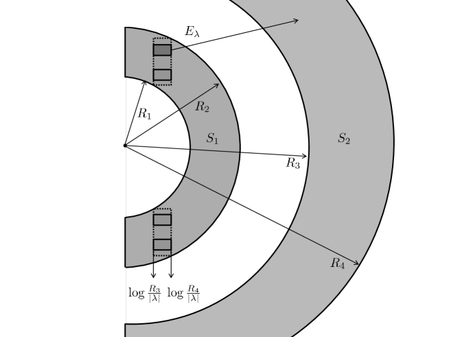
Figure 1. The set $E_{\lambda}^{-1}(S_{2})\cap S_{1}$. One preimage component of $S_{2}$ is shown with a slightly darker background. The two rectangles constructed in the proof of Lemma 2.1 are shown with a dashed boundary. Note that $R_{3}$ is not necessarily larger than $R_{2}$.

Lemma 2.1.

Suppose that $0<R_{1}<R_{2}$ and $0<R_{3}<R_{4}$ are such that

(2.2) $$R_{2}>\max\left\{2R_{1},\ R_{1}+16\pi,\ 3\log\frac{R_{4}}{|\lambda|}\right\},$$

and

(2.3) $$R_{3}>|\lambda|.$$

Let $S_{1}={H(R_{1},R_{2})}$, $S_{2}={H(R_{3},R_{4})}$, and let $D$ be the union of all the components of $E_{\lambda}^{-1}(S_{2})$ which are contained in $S_{1}$. Then

(2.4) $$\operatorname{dens}(D,S_{1})\geq\frac{1}{2\pi R_{2}}\log\frac{R_{4}}{R_{3}}.$$

Proof.

Each component of $E_{\lambda}^{-1}(S_{2})$ is a rectangle of the form, for $n\in\mathbb{Z}$,

(2.5) $$\left\{z:\log\frac{R_{3}}{|\lambda|}\leq\operatorname{Re}(z)\leq\log\frac{R_{4}}{|\lambda|},\ \left(2n-\frac{1}{2}\right)\pi\leq\operatorname{Im}(z)+\arg(\lambda)\leq\left(2n+\frac{1}{2}\right)\pi\right\}.$$

Suppose that the inequalities (2.2) and (2.3) both hold. Consider two large rectangles, each with sides parallel to the coordinate axes. One rectangle has a vertex at the point in the upper half-plane where the vertical line $\{z:\operatorname{Re}(z)=\log\frac{R_{3}}{|\lambda|}\}$ meets the circle $B(0,R_{1})$; note that if $R_{1}\leq\log\frac{R_{3}}{|\lambda|}$ we put this vertex at $R_{1}$. The diagonally opposite vertex of this rectangle is at the point in the upper half-plane where the vertical line $\{z:\operatorname{Re}(z)=\log\frac{R_{4}}{|\lambda|}\}$ meets the circle $B(0,R_{2})$. The second rectangle is the complex conjugate of the first one.

Let $h$ be the height of each rectangle. It follows by an application of Pythagoras’s theorem to this rectangle, and by (2.2), that

$$h =\left(R_{2}^{2}-\left(\log\frac{R_{4}}{|\lambda|}\right)^{2}\right)^{\frac{1}{2}}-\left(\max\left\{0,\ R_{1}^{2}-\left(\log\frac{R_{3}}{|\lambda|}\right)^{2}\right\}\right)^{\frac{1}{2}}$$

$$\geq\frac{7}{8}R_{2}-R_{1}\geq\frac{3}{4}(R_{2}-R_{1}).$$

It follows by (2.2) and (2.5) that each rectangle contains at least $\frac{1}{4\pi}(R_{2}-R_{1})$ components of $E_{\lambda}^{-1}(S_{2})$. Hence $S_{1}$ contains at least $\frac{1}{2\pi}(R_{2}-R_{1})$ components of $E_{\lambda}^{-1}(S_{2})$, each of which is a closed rectangle of height $\pi$ and width at least $\log\frac{R_{4}}{R_{3}}$. Equation (2.4) follows from this, and the fact that area$(S_{1})=\frac{1}{2}\pi(R_{2}^{2}-R_{1}^{2})$. ∎

For a domain $V$ and a transcendental entire function $f$, univalent in $V$, we define the distortion of $f$ in $V$ by

(2.6) $$D_{V}(f)=\frac{\sup_{z\in V}|f^{\prime}(z)|}{\inf_{z\in V}|f^{\prime}(z)|}.$$

For functions in the exponential family, the following facts are immediate.

Lemma 2.2.

Suppose that $F$ is a set such that $\inf\{|z|:z\in F\}=r_{1}>0$ and $\sup\{|z|:z\in F\}=r_{2}$, and that $V$ is a component of $E_{\lambda}^{-1}(F)$ such that $E_{\lambda}$ is univalent in $V$. Then

(2.7) $$|E_{\lambda}^{\prime}(z)|\geq r_{1},\quad\text{for }z\in V,$$

and

(2.8) $$D_{V}(E_{\lambda})=\frac{r_{2}}{r_{1}}.$$

We also use two well-known properties of Hausdorff dimension. For the first see, for example, [13].

Lemma 2.3.

Suppose that $(F)_{i\in I}$ is a collection of subsets of $\mathbb{C}$, and that $I$ is a finite or countable set. Then

$$\dim_{H}\bigcup_{i\in I}F_{i}=\sup_{i\in I}\ \{\dim_{H}F_{i}\}.$$

The second property is used frequently but we are not aware of a reference.

Lemma 2.4.

Suppose that $f$ is a non-constant transcendental entire function and that $U\subset\mathbb{C}$. Then

$$\dim_{H}f(U)=\dim_{H}f^{-1}(U)=\dim_{H}U.$$

3. A lower bound on the Hausdorff dimension

In this section we prove the following theorem which gives a lower bound on the Hausdorff dimension of $I_{R}(\underline{t})$ for a certain type of annular itinerary.

Theorem 3.1.

Suppose that $\lambda\neq 0$. Then there exists $R_{0}=R_{0}(\lambda)>1$ such that, if $R\geq R_{0}$ and $\underline{t}$ is an escaping, non-zero, admissible and slowly-growing annular itinerary, then $\dim_{H}I_{R}(\underline{t})\geq 1.$

To prove Theorem 3.1, we use a well-known construction and result of McMullen. Let $(\mathcal{E}_{n})_{n\geq 0}$ be a sequence of finite collections of pairwise disjoint compact subsets of $\mathbb{C}$ such that the following both hold:

1. If $F\in\mathcal{E}_{n+1}$, then there exists a unique $G\in\mathcal{E}_{n}$ such that $F\subset G$;

2. If $G\in\mathcal{E}_{n}$, then there exists at least one $F\in\mathcal{E}_{n+1}$ such that $G\supset F$.

We write

(3.1) $$D_{n}=\bigcup_{F\subset\mathcal{E}_{n}}F,\text{ for }n\geq 0,\quad\text{and}\quad D=\bigcap_{n\geq 0}D_{n}.$$

McMullen’s result is the following [17, Proposition 2.2]. Here, for a set $U$, $\operatorname{diam}U$ denotes the Euclidean diameter of $U$.

Lemma 3.1.

Suppose that there exists a sequence of finite collections of pairwise disjoint compact sets, $(\mathcal{E}_{n})_{n\geq 0}$, which satisfies conditions (i) and (ii) above, and let $D$ and $(D_{n})_{n\geq 0}$ be as defined in (3.1). Suppose also that $(\Delta_{n})_{n\geq 0}$ and $(d_{n})_{n\geq 0}$ are sequences of positive real numbers, with $d_{n}\rightarrow 0$ as $n\rightarrow\infty$, such that, for each $n\geq 0$ and for each $F\in\mathcal{E}_{n}$, we have

$$\operatorname{dens}(D_{n+1},F)\geq\Delta_{n}\quad\text{and}\quad\operatorname{diam}F\leq d_{n}.$$

Then

(3.2) $$\dim_{H}D\geq 2-\limsup_{n\rightarrow\infty}\frac{\sum_{m=0}^{n}|\log\Delta_{m}|}{|\log d_{n}|}.$$

Remark 3.

In [17] the upper bound of summation in (3.2) was given as $n+1$. However, the stronger result (3.2) – which is required in the proof of Theorem 3.1 – follows from McMullen’s proof, and has been given in, for example, [4, Lemma 4.4] and [24, Lemma 4.3].

We also use the following. This is a version of [23, Lemma 5.2], which itself is a detailed version of [17, Proposition 3.1].

Lemma 3.2.

Suppose that $f$ is a transcendental entire function, and there exists a set $U\subset\mathbb{C}$ and constants $\alpha>1$ and $M>0$ such that

(3.3) $$|f^{\prime}(z)|>\alpha\quad\text{ and }\quad\left|\frac{f^{\prime\prime}(z)}{f^{\prime}(z)}\right|<M,\quad\text{for }z\in U.$$

Suppose also that there exists $s\in(0,(4M)^{-1})$ such that if $B\subset U$ is a disc of diameter $s$, then $f$ is conformal in a neighbourhood of $B$. Suppose finally that $(B_{m})_{m\in\{1,2,\ldots,n\}}$ is a sequence of sets contained in $U$, each of diameter less than $s$, and such that

$$B_{m+1}\subset f(B_{m}),\quad\text{for }m\in\{1,2,\ldots,n-1\}.$$

For $m\in\{1,2,\ldots,n\}$, let $\phi_{m}$ be the inverse branch of $f$ which maps $f(B_{m})$ to $B_{m}$, and set $V=\phi_{1}\circ\phi_{2}\circ\cdots\circ\phi_{n}(f(B_{n}))$. Then there exists $\tau=\tau(M,s,\alpha)>1$ such that

$$D_{V}(f^{n})\leq\tau.$$

Note that in [23, Lemma 5.2] the sets $B_{n}$ are squares of side $s$. The proof of the above result follows in exactly the same way, and is omitted.

We deduce the following.

Corollary 3.1.

There exist absolute constants $s_{0}>0$ and $\tau_{0}>1$ such that the following holds. Suppose that $\lambda\neq 0$, $n\in\mathbb{N}$ and $V$ is a set such that

$$E_{\lambda}^{m}(V)\subset\left\{z:\operatorname{Re}(z)>\log\frac{2}{|\lambda|}\right\}\text{ and }\operatorname{diam}E_{\lambda}^{m}(V)<s_{0},\quad\text{for }0\leq m<n.$$

Then $D_{V}(E_{\lambda}^{n})\leq\tau_{0}$.

Proof.

This result follows from Lemma 3.2 with $f=E_{\lambda}$ , $U=\left\{z:\operatorname{Re}(z)>\log\frac{2}{|\lambda|}\right\}$, $\alpha=M=2$, and $B_{m}=E_{\lambda}^{m-1}(V)$, for $1\leq m\leq n$. ∎

We now give the proof of Theorem 3.1. Roughly speaking, our method of proof is as follows. First we set a value of $R_{0}$ sufficiently large to enable us to use Lemma 2.1. We then define a set which is contained in $I_{R}(\underline{t})$ and apply McMullen’s result to obtain a lower bound on the Hausdorff dimension of this set.

Proof of Theorem 3.1.

Let $s_{0}$ be the constant in Corollary 3.1. We choose

(3.4) $$R_{0}>\max\left\{e,|\lambda|,\frac{2}{s_{0}}\right\},$$

sufficiently large that

(3.5) $$R(R-1)>16\pi+2\quad\text{ and }\quad R>3\log\frac{R^{2}}{|\lambda|}+1,\quad\text{for }R\geq R_{0}.$$

Suppose that $R\geq R_{0}$, and that $\underline{t}$ is an escaping, non-zero, admissible and slowly-growing annular itinerary. To use Lemma 3.1 we need to work with compact and disjoint sets. In order to do this, and recalling the definition (2.1), we define disjoint closed half-annuli

$$H_{n}=H(R^{n}+1,R^{n+1}-1),\quad\text{for }n\in\mathbb{N}.$$

Since $\underline{t}$ is admissible and non-zero, we deduce by (3.4) and (3.5) that, for $n\geq 0$, we have

(3.6) $$R^{t_{n}+1}>Re^{t_{n}}>Rt_{n+1}>3t_{n+1}\log R+3\log\frac{R}{|\lambda|}+1>3\log\left(\frac{R^{t_{n+1}+1}-1}{|\lambda|}\right)+1.$$

Since $\underline{t}$ is non-zero, we deduce from (3.4), (3.5) and (3.6) that the hypotheses of Lemma 2.1 are satisfied with $S_{1}=H_{t_{n}}$ and $S_{2}=H_{t_{n+1}}$, for $n\geq 0$.

In order to use Lemma 3.1, we define a sequence of finite collections of pairwise disjoint compact sets as follows. First set

$$\mathcal{E}_{0}=\{H_{t_{0}}\},$$

and, for $n\geq 0$,

$$\mathcal{E}_{n+1}=\{F:F\subset G,\text{ for some }G\in\mathcal{E}_{n},\text{ and }E_{\lambda}^{n+1}(F)=H_{t_{n+1}}\}.$$

Let $D_{n}$, for $n\geq 0$, and $D$ be the sets defined in (3.1). It follows from (3.1) that $D\subset I_{R}(\underline{t}).$ It is sufficient, therefore, to show that $\dim_{H}D\geq 1$.

It follows from Lemma 2.1 that the conditions (i) and (ii) stated prior to Lemma 3.1 are both satisfied. It remains to estimate the diameters and the densities stated in Lemma 3.1. Note that to apply equation (3.2) we may omit the definition of a finite number of these estimates.

Since $\underline{t}$ is escaping, we can let $N_{0}\geq 2$ be sufficiently large that $t_{n-1}\geq 2$, for $n\geq N_{0}$. Suppose that $n\geq N_{0}$ and that $F\in\mathcal{E}_{n}$. Note that $E_{\lambda}^{n}(F)=H_{t_{n}}$. We first find an upper bound on the diameter of $F$. Since

$$\text{diam }E_{\lambda}^{n}(F)=\text{diam }H_{t_{n}}<2R^{t_{n}+1},$$

we have, by (2.7), that

(3.7) $$\operatorname{diam}F\leq 2R^{t_{n}+1}\frac{1}{R^{t_{1}}}\frac{1}{R^{t_{2}}}\cdots\frac{1}{R^{t_{n}}}=2R^{1-\sum_{m=1}^{n-1}t_{m}}.$$

We set $d_{n}=2R^{1-\sum_{m=1}^{n-1}t_{m}}$. Since $\underline{t}$ is escaping, we deduce that

(3.8) $$d_{n}\rightarrow 0\quad\text{and}\quad|\log d_{n}|=\log R\ \sum_{m=1}^{n-1}t_{m}\left(1+o(1)\right)\text{ as }n\rightarrow\infty.$$

We next show that the distortion of $E_{\lambda}^{n}$ on $F$ is bounded independently of $n$ and $F$. Once again by (2.7), and by (3.4), we have

$$\operatorname{diam}E_{\lambda}^{m}(F)\leq 2R^{t_{n}+1}\frac{1}{R^{t_{n-1}}}\frac{1}{R^{t_{n}}}\leq\frac{2}{R}<s_{0},\quad\text{for }0\leq m<n-1.$$

Suppose that $0\leq m<n-1$ and that $z\in E_{\lambda}^{m}(F)$. Since $\underline{t}$ is non-zero, we have $|E_{\lambda}(z)|\geq R$. We deduce by (3.4) that

$$\operatorname{Re}(z)\geq\log\frac{R}{|\lambda|}>\log\frac{2}{|\lambda|}.$$

Hence

$$E_{\lambda}^{m}(F)\subset\left\{z:\operatorname{Re}(z)>\log\frac{2}{|\lambda|}\right\},\quad\text{for }0\leq m<n-1.$$

We deduce by Corollary 3.1 that $D_{F}(E_{\lambda}^{n-1})\leq\tau_{0}$. Moreover, it follows from (2.8) that $D_{E_{\lambda}^{n-1}(F)}(E_{\lambda})\leq R$. Thus

(3.9) $$D_{F}(E_{\lambda}^{n})\leq D_{F}(E_{\lambda}^{n-1})\ D_{E_{\lambda}^{n-1}(F)}(E_{\lambda})\leq\tau_{0}R.$$

We use (3.9) to find a lower bound on dens$(D_{n+1},F)$. Note that $E_{\lambda}^{n}(D_{n+1})$ consists of those components of $E_{\lambda}^{-1}(H_{t_{n+1}})$ which are contained in $H_{t_{n}}$. Hence, by (2.4), (3.4) and (3.9), we have

$$\operatorname{dens}(D_{n+1},F) \geq\frac{1}{(\tau_{0}R)^{2}}\operatorname{dens}(E_{\lambda}^{n}(D_{n+1}),E_{\lambda}^{n}(F))$$

$$\geq\frac{1}{(\tau_{0}R)^{2}}\frac{1}{2\pi\left(R^{t_{n}+1}-1\right)}\log\frac{R^{t_{n+1}+1}-1}{R^{t_{n+1}}+1}$$

$$\geq\frac{\log R}{4\tau_{0}^{2}\pi R^{t_{n}+3}}.$$

We set $\Delta_{n}=\frac{\log R}{4\tau_{0}^{2}\pi R^{t_{n}+3}}$. Note that

(3.10) $$|\log\Delta_{n}|=t_{n}\log R\left(1+o(1)\right)\text{ as }n\rightarrow\infty.$$

Since $\underline{t}$ is escaping and slowly-growing, it follows, by (1.8), (3.8) and (3.10), that

$$\limsup_{n\rightarrow\infty}\frac{\sum_{m=0}^{n}|\log\Delta_{m}|}{|\log d_{n}|} =\limsup_{n\rightarrow\infty}\frac{\log R\ \sum_{m=1}^{n}t_{m}(1+o(1))}{\log R\ \sum_{m=1}^{n-1}t_{m}(1+o(1))}$$

$$=\limsup_{n\rightarrow\infty}\left(\frac{t_{n}(1+o(1))}{\sum_{m=1}^{n-1}t_{m}(1+o(1))}+\frac{\sum_{m=1}^{n-1}t_{m}(1+o(1))}{\sum_{m=1}^{n-1}t_{m}(1+o(1))}\right)$$

$$=1.$$

We deduce by Lemma 3.1 that $\dim_{H}D\geq 1$, as required.∎

4. An upper bound on Hausdorff dimension

In this section we prove a theorem which gives an upper bound on the Hausdorff dimension of certain sets, and so is, in a sense, complementary to Theorem 3.1. First we define the sets. Suppose that, for each $p\in\mathbb{N}$, $(g_{p,n})_{n\in\mathbb{N}}$ and $(h_{p,n})_{n\in\mathbb{N}}$ are sequences of positive real numbers such that

(4.1) $$h_{p,n}\geq g_{p,n},\quad\text{for }n\in\mathbb{N}.$$

For $\lambda\neq 0$ define the set $T_{g,h}$ by

(4.2) $$T_{g,h}=\{z:\text{there exist }N,p\in\mathbb{N}\text{ s.t. }E_{\lambda}^{n}(z)\in A(g_{p,n},h_{p,n}),\text{ for }n\geq N\}.$$

Our theorem is as follows.

Theorem 4.1.

Suppose that $\lambda\neq 0$, and that for each $p\in\mathbb{N}$, $(g_{p,n})_{n\in\mathbb{N}}$ and $(h_{p,n})_{n\in\mathbb{N}}$ are sequences of positive real numbers such that (4.1) is satisfied,

(4.3) $$g_{p,n}\rightarrow\infty\text{ as }n\rightarrow\infty,$$

and

(4.4) $$\frac{\log g_{p,n}}{\log^{+}\log h_{p,n+1}}\rightarrow\infty\text{ as }n\rightarrow\infty.$$

Then $\dim_{H}T_{g,h}\leq 1.$

Proof.

Choose

(4.5) $$\beta>\max\left\{\sqrt{1+\pi^{2}},\ \frac{1}{s_{0}}\right\}$$

and set

$$c_{0}=|\lambda|e^{1+\beta}\max\left\{\frac{2}{|\lambda|},\ \exp(\beta^{2})\right\}$$

and

(4.6) $$c_{1}=\log\frac{c_{0}}{|\lambda|}=1+\beta+\max\left\{\log\frac{2}{|\lambda|},\ \beta^{2}\right\},$$

where $s_{0}$ is the constant in Corollary 3.1. By (4.3), for each $p\in\mathbb{N}$ we can choose $\ell_{p}\in\mathbb{N}$ such that

(4.7) $$g_{p,n}>c_{0},\quad\text{for }n\geq\ell_{p}.$$

Define sets

(4.8) $$S_{\nu,p}=\{z:E_{\lambda}^{n}(z)\in A(g_{p,\nu+n},h_{p,\nu+n}),\text{ for }n\geq 0\},\quad\text{for }\nu,p\in\mathbb{N}.$$

Fix a value of $p\in\mathbb{N}$, and suppose that $\nu\geq\ell_{p}$. We claim that

(4.9) $$\dim_{H}S_{\nu,p}\leq 1.$$

Before proving (4.9) we show that the result of the lemma can be deduced from this equation. First we claim that

(4.10) $$T_{g,h}\subset\bigcup_{p\in\mathbb{N}}\bigcup_{\nu\geq\ell_{p}}E_{\lambda}^{-\nu}(S_{\nu,p}).$$

For, suppose that $z\in T_{g,h}$, in which case there exist $N,p\in\mathbb{N}$ such that

$$E_{\lambda}^{n}(z)~{}\in~{}A(g_{p,n},h_{p,n}),\quad\text{for }n\geq N.$$

It follows that there exists $\nu\geq\max\{N,\ell_{p}\}$ such that $E_{\lambda}^{n}(E_{\lambda}^{\nu}(z))\in A(g_{p,n+\nu},h_{p,n+\nu})$, for $n\geq 0$, and so $E_{\lambda}^{\nu}(z)\in S_{\nu,p}$. This establishes equation (4.10). Theorem 4.1 follows from (4.9) and (4.10), by Lemma 2.3 and Lemma 2.4.

If remains to show that (4.9) holds for $\nu\geq\ell_{p}$. We establish this result using a sequence of covers of $S_{\nu,p}$ and basic properties of Hausdorff dimension. We suppress the variable $p$ for simplicity.

First we note some properties of $S_{\nu}$ and then use these properties to define a sequence of covers of this set. It follows from (4.7), and the fact that $\nu\geq\ell$, that

$$|E_{\lambda}(E_{\lambda}^{n}(z))|=|\lambda|e^{\operatorname{Re}(E_{\lambda}^{n}(z))}>c_{0},\quad\text{for }z\in S_{\nu},\ n\geq 0.$$

We deduce by (4.6) that

(4.11) $$\operatorname{Re}(E_{\lambda}^{n}(z))>\log\frac{c_{0}}{|\lambda|}=c_{1},\quad\text{for }z\in S_{\nu},\ n\geq 0.$$

Define compact sets

(4.12) $$W_{n,m}=A(e^{m-1}g_{n},e^{m}g_{n})\cap\{z:\operatorname{Re}(z)\geq c_{1}\},\quad\text{for }n,m\in\mathbb{N}.$$

We observe that each component of $E_{\lambda}^{-1}(W_{n,m})$, for $m,n\in\mathbb{N}$, is contained in a distinct rectangle of the form,

(4.13) $$\left\{z:-1\leq\operatorname{Re}(z)-m-\log g_{n}+\log|\lambda|\leq 0,\ -\pi/2\leq\operatorname{Im}(z)+\arg(\lambda)+2k\pi\leq\pi/2\right\},$$

for some $k\in\mathbb{Z}$. Hence, by (4.5), if $F$ is a component of $E_{\lambda}^{-1}(W_{n,m})$, then

(4.14) $$\operatorname{diam}F\leq\beta,\quad\text{for }m,n\in\mathbb{N}.$$

For simplicity of notation, define sets of integers

(4.15) $$\alpha_{n}=\left\{1,2,\ldots,\left[\log\frac{h_{n}}{g_{n}}\right]+1\right\},\quad\text{for }n\in\mathbb{N},$$

where $[x]$ denotes the integer part of $x$. Note that

(4.16) $$A(g_{n},h_{n})\cap\{z:\operatorname{Re}(z)\geq c_{1}\}\subset\bigcup_{m\in\alpha_{n}}W_{n,m},\quad\text{for }n\in\mathbb{N}.$$

Now set

$$\mathcal{E}_{0}=\{W_{\nu,m}:m\in\alpha_{\nu}\},$$

and, for $n\geq 0$,

$$\mathcal{E}_{n+1}=\{F:E_{\lambda}^{n+1}(F)=W_{\nu+n+1,m}\text{ for some }m\in\alpha_{\nu+n+1}\text{ and }F\ \cap\ G\neq\emptyset\text{ for some }G\in\mathcal{E}_{n}\}.$$

It follows by (4.11) and (4.16) that

$$S_{\nu}\subset\bigcup_{F\in\mathcal{E}_{n}}F,\quad\text{for }\text{each }n\geq 0.$$

This completes the definition of the sequence of covers of $S_{\nu}$.

Next we study the properties of the sets in these covers, particularly the diameters of these sets. Suppose that $q\in\mathbb{N}$. We claim that the following hold for $n\geq q$ and $F\in\mathcal{E}_{n}$;

(4.17) $$\operatorname{diam}E_{\lambda}^{n-q}(F)\leq\beta^{3-2q},$$

(4.18) $$E_{\lambda}^{n-q}(F)\subset\left\{z:\operatorname{Re}(z)\geq c_{1}-\sum_{k=1}^{q}\beta^{3-2k}\right\},$$

and

(4.19) $$E_{\lambda}^{n-q}(F)\subset\left\{z:\operatorname{Re}(z)>\max\left\{\log\frac{2}{|\lambda|},\beta^{2}\right\}\right\}.$$

First we note that (4.19) follows from (4.5), (4.6) and (4.18).

We prove (4.17) and (4.18) by induction on $q$. We consider first the case that $q=1$. Suppose that $n\in\mathbb{N}$ and that $F\in\mathcal{E}_{n}$. By (4.14), $E_{\lambda}^{n-1}(F)$ has diameter at most $\beta$. Moreover, since

$$E_{\lambda}^{n-1}(F)\cap W_{\nu+n-1,m^{\prime}}\neq\emptyset,\quad\text{for }\text{some }m^{\prime}\in\alpha_{\nu+n-1},$$

we deduce by (4.12) that $E_{\lambda}^{n-1}(F)\subset\{z:\operatorname{Re}(z)\geq c_{1}-\beta\}$. This establishes (4.17) and (4.18) in the case that $q=1$.

Now, suppose that (4.17) and (4.18) have been been established for $1\leq q\leq s$, for some $s\in\mathbb{N}$. Suppose that $n\geq s+1$, that $F\in\mathcal{E}_{n}$ and that $G\in\mathcal{E}_{n-1}$ is such that $F\cap G\neq\emptyset$. First, we deduce by (2.7), and by (4.17) and (4.19) with $s$ in place of $q$, that

(4.20) $$\operatorname{diam}E_{\lambda}^{n-(s+1)}(F)\leq\frac{\operatorname{diam}E_{\lambda}^{n-s}(F)}{\inf\{|z|:z\in E_{\lambda}^{n-s}(F)\}}\leq\frac{\beta^{3-2s}}{\beta^{2}}=\beta^{3-2(s+1)}.$$

Second, applying (4.18) with $G$ in place of $F$, $n-1$ in place of $n$, and $s$ in place of $q$, we deduce that

$$E_{\lambda}^{(n-1)-s}(G)\subset\left\{z:\operatorname{Re}(z)\geq c_{1}-\sum_{k=1}^{s}\beta^{3-2k}\right\}.$$

Since $E_{\lambda}^{n-(s+1)}(F)\cap E_{\lambda}^{(n-1)-s}(G)\neq\emptyset$, it follows by (4.20) that

$$E_{\lambda}^{n-(s+1)}(F)\subset\left\{z:\operatorname{Re}(z)\geq c_{1}-\sum_{k=1}^{s}\beta^{3-2k}-\beta^{3-2(s+1)}\right\}.$$

By induction, this completes the proof of (4.17) and (4.18). We observe that it follows from (4.17) that the diameters of the sets in $\mathcal{E}_{n}$ tend uniformly to zero as $n\rightarrow\infty$.

Suppose next that $\epsilon>0$. By the definition of Hausdorff dimension, together with the observation above regarding the diameters of the sets in $\mathcal{E}_{n}$, our proof of (4.9) is complete if we can show that

$$\sum_{F\in\mathcal{E}_{n+1}}(\text{diam }F)^{1+\epsilon}\leq\sum_{F\in\mathcal{E}_{n}}(\text{diam }F)^{1+\epsilon},\quad\text{for }\text{large }n,$$

or indeed if we can show that, for all sufficiently large $n$, we have for each $G\in\mathcal{E}_{n}$ that

(4.21) $$\sum_{\begin{subarray}{c}F\in\mathcal{E}_{n+1},\\ F\cap G\neq\emptyset\end{subarray}}\left(\frac{\text{diam }F}{\text{diam }G}\right)^{1+\epsilon}\leq 1.$$

Suppose that $n\in\mathbb{N}$ and that $G\in\mathcal{E}_{n}$, in which case $E_{\lambda}^{n}(G)=W_{\nu+n,m}$, for some $m\in\alpha_{\nu+n}$. Suppose also that $F~{}\in~{}\mathcal{E}_{n+1}$ intersects with $G$, in which case $E_{\lambda}^{n}(F)$ intersects with $W_{\nu+n,m}$ and is a preimage component of $W_{\nu+n+1,m^{\prime}}$, for some $m^{\prime}\in\alpha_{\nu+n+1}$.

We note the following two simple estimates. First, it follows from (4.13) that for each $m^{\prime}\in\alpha_{\nu+n+1}$, there are at most $O(e^{m}g_{\nu+n})$ preimage components of $W_{\nu+n+1,m^{\prime}}$ which intersect with $W_{\nu+n,m}$. It follows from this estimate and from (4.15), that the total number of elements of $\mathcal{E}_{n+1}$ which intersect with $G$ is at most

(4.22) $$O\left(e^{m}g_{\nu+n}\log\frac{h_{\nu+n+1}}{g_{\nu+n+1}}\right)\text{ as }n\rightarrow\infty.$$

Second, it is immediate that

(4.23) $$(\operatorname{diam}E_{\lambda}^{n}(G))^{-1}=O((e^{m}g_{\nu+n})^{-1})\text{ as }n\rightarrow\infty.$$

Next we estimate the distortion of $E_{\lambda}^{n}$ in $F\cup G$. Suppose that $n\geq 2$. We deduce by (4.5) and (4.17) that

$$\operatorname{diam}E_{\lambda}^{m}(G)<s_{0},\quad\text{for }0\leq m<n-1.$$

It follows by (4.19) and Corollary 3.1 that $D_{G}(E_{\lambda}^{n-1})\leq\tau_{0}$. Moreover, it follows from (2.8) that $D_{E_{\lambda}^{n-1}(G)}(E_{\lambda})\leq e$. We deduce that $D_{G}(E_{\lambda}^{n})=O(1)\text{ as }n\rightarrow\infty$. By a similar argument $D_{F}(E_{\lambda}^{n})=O(1)\text{ as }n\rightarrow\infty$. Hence, since $F\cap G\neq\emptyset$, we have

(4.24) $$D_{F\cup G}(E_{\lambda}^{n})=O(1)\text{ as }n\rightarrow\infty.$$

Combining these estimates, we deduce from (4.14), (4.22), (4.23) and (4.24) that

$$\sum_{\begin{subarray}{c}F\in\mathcal{E}_{n+1},\\ F\cap G\neq\emptyset\end{subarray}}\left(\frac{\text{diam }F}{\text{diam }G}\right)^{1+\epsilon} \leq O(1)\sum_{\begin{subarray}{c}F\in\mathcal{E}_{n+1},\\ F\cap G\neq\emptyset\end{subarray}}\left(\frac{\text{diam }E_{\lambda}^{n}(F)}{\text{diam }E_{\lambda}^{n}(G)}\right)^{1+\epsilon}$$

$$=O\left(e^{m}g_{\nu+n}\log\frac{h_{\nu+n+1}}{g_{\nu+n+1}}.(e^{m}g_{\nu+n})^{-(1+\epsilon)}\right)$$

$$\leq O\left(g_{\nu+n}^{-\epsilon}\log h_{\nu+n+1}\right).$$

We deduce by (4.4) that (4.21) holds, as required. ∎

5. Dimension results

In this section we prove Theorem 1.2, Theorem 1.3, Theorem 1.4 and Theorem 1.5. In each case we use Theorem 3.1 to show that the Hausdorff dimension is bounded below by $1$, and we use Theorem 4.1 to show that the Hausdorff dimension is bounded above by $1$. It is somewhat simpler to prove Theorem 1.3 before Theorem 1.2.

Proof of Theorem 1.3.

Choose $R\geq R_{0}$, where $R_{0}$ is as in the statement of Theorem 3.1, and let $\underline{t}$ be the sequence

(5.1) $$\underline{t}=1\ 1\ 1\ 2\ 3\ \ldots\ (n-1)\ \ldots.$$

We deduce by Theorem 3.1 that $\dim_{H}I_{R}(\underline{t})\geq 1$. Suppose that $z\in I_{R}(\underline{t})$, in which case $R^{n-1}\leq|E_{\lambda}^{n}(z)|\leq R^{n}$, for $n\geq 2$. It follows that $z\in L_{A}(E_{\lambda})$. Hence $I_{R}(\underline{t})\subset L_{A}(E_{\lambda})$, and so $\dim_{H}L_{A}(E_{\lambda})\geq 1$.

Next, for each $p\in\mathbb{N}$, let sequences $(g_{p,n})_{n\in\mathbb{N}}$ and $(h_{p,n})_{n\in\mathbb{N}}$ be defined by

(5.2) $$g_{p,n}=n^{\log^{+p}(n)}\text{ and }h_{p,n}=e^{pn},\quad\text{for }n\in\mathbb{N}.$$

We deduce by Theorem 4.1 that $\dim_{H}T_{g,h}\leq 1$. Suppose that $z\in L_{A}(E_{\lambda})$, in which case, by (1.5), there exist $p,N\in\mathbb{N}$ and $R>1$ such that

$$n^{\log^{+p}(n)}\leq|E_{\lambda}^{n}(z)|\leq R^{n},\quad\text{for }n\geq N.$$

If $p$ is sufficiently large, then $R^{n}\leq e^{pn}$, for $n\in\mathbb{N}$. We deduce that $z\in T_{g,h}$, where $g,h$ are as defined in (5.2). It follows that $L_{A}(E_{\lambda})\subset T_{g,h}$, and so $\dim_{H}L_{A}(E_{\lambda})\leq 1$. This completes the proof of Theorem 1.3. ∎

Proof of Theorem 1.2.

Choose $R\geq R_{0}$, where $R_{0}$ is as in the statement of Theorem 3.1, and let $\underline{t}$ be as defined in (5.1). Recall that $\dim_{H}I_{R}(\underline{t})\geq 1$. We deduce Theorem 1.2 from Theorem 1.3 and the fact that $I_{R}(\underline{t})\subset L_{U}(E_{\lambda})\subset L_{A}(E_{\lambda}).$ ∎

Proof of Theorem 1.4.

Choose $R\geq R_{0}$, where $R_{0}$ is as in the statement of Theorem 3.1, and let $\underline{t^{\prime}}$ be the sequence

$$\underline{t^{\prime}}=1\ 4\ 9\ \ldots\ (n+1)^{2}\ \ldots.$$

We deduce by Theorem 3.1 that $\dim_{H}I_{R}(\underline{t^{\prime}})\geq 1$. Suppose that $z\in I_{R}(\underline{t^{\prime}})$, in which case $R^{(n+1)^{2}}\leq|E_{\lambda}^{n}(z)|\leq R^{(n+1)^{2}+1}$, for $n\geq 0$. It follows that $z\in M_{A}(E_{\lambda})$. Hence $I_{R}(\underline{t^{\prime}})\subset M_{A}(E_{\lambda})$, and so $\dim_{H}M_{A}(E_{\lambda})\geq 1$.

Next, for each $p\in\mathbb{N}$, let sequences $(g^{\prime}_{p,n})_{n\in\mathbb{N}}$ and $(h^{\prime}_{p,n})_{n\in\mathbb{N}}$ be defined by

(5.3) $$g^{\prime}_{p,n}=e^{n\log^{+p}(n)}\text{ and }h^{\prime}_{p,n}=\exp(e^{pn}),\quad\text{for }n\in\mathbb{N}.$$

We deduce by Theorem 4.1 that $\dim_{H}T_{g^{\prime},h^{\prime}}\leq 1$.

Suppose that $z\in M_{A}(E_{\lambda})$, in which case, by (1.6), there exist $p,N\in\mathbb{N}$ and $R>1$ such that

$$e^{n\log^{+p}(n)}\leq|E_{\lambda}^{n}(z)|\leq\exp(e^{pn}),\quad\text{for }n\geq N.$$

We deduce that $z\in T_{g^{\prime},h^{\prime}}$, where $g^{\prime},h^{\prime}$ are as defined in (5.3). It follows that $M_{A}(E_{\lambda})\subset T_{g^{\prime},h^{\prime}}$, and so $\dim_{H}M_{A}(E_{\lambda})\leq 1$. This completes the proof of Theorem 1.4. ∎

Finally we prove Theorem 1.5.

Proof of Theorem 1.5.

Suppose that $f$ is a transcendental entire function, $R>1$ and $\underline{t}=t_{0}t_{1}t_{2}\ldots$ is an escaping annular itinerary. For each $p\in\mathbb{N}$ we define sequences $(g_{p,n})_{n\in\mathbb{N}}$ and $(h_{p,n})_{n\in\mathbb{N}}$ by $g_{p,n}=R^{t_{n}},\text{ and }h_{p,n}=R^{t_{n}+1}.$ We deduce by Theorem 4.1 that $\dim_{H}T_{g,h}\leq 1$. The first part of the theorem follows since $I_{R}(\underline{t})\subset T_{g,h}$.

The second part of Theorem 1.5 is an immediate consequence of this, together with Theorem 3.1. ∎

6. The uniformly slowly escaping set

In this section, for a general transcendental entire function $f$, we give two results on the set $L_{U}(f)$. First, we give a necessary and sufficient condition for $L_{U}(f)$ to be non-empty. Here $m(r,f)=\min_{|z|=r}|f(z)|$ denotes the minimum modulus of $f$, for $r>0$.

Theorem 6.1.

Suppose that $f$ is a transcendental entire function. Then

$$L_{U}(f)\cap J(f)\neq\emptyset$$

if and only if there exist positive constants $c$ and $r_{0}$, and $d>1$ such that

(6.1) $$\text{for all }r\geq r_{0}\text{ there exists }\rho\in(r,dr)\text{ such that }m(\rho,f)\leq c.$$

Moreover, if $L_{U}(f)\neq\emptyset$, then $L_{U}(f)\cap J(f)\neq\emptyset$.

Remark 4.

The condition (6.1) was used in [21], also in relation to points tending to infinity at a specified rate. As observed in [21], this condition holds whenever $f$ is bounded on a path to infinity. It is well-known that this is the case for functions in the class $\mathcal{B}$ in particular.

Second, we show that when $L_{U}(f)$ is not empty, it has a number of familiar properties which show that, in general, this is a dynamically interesting set. We say that a set $S$ is completely invariant if $z\in S$ implies that $f(z)\in S$ and also that $f^{-1}(\{z\})\subset S$.

Theorem 6.2.

Suppose that $f$ is a transcendental entire function, and that $L_{U}(f)~{}\neq~{}\emptyset$. Then the following all hold.

1. $L_{U}(f)$ is completely invariant;

2. If $U$ is a Fatou component of $f$ and $U\cap L_{U}(f)\neq\emptyset$, then $U\subset L_{U}(f)$;

3. $L_{U}(f)$ is dense in $J(f)$ and $J(f)=\partial$$L_{U}(f)$.

Remark 5.

An example of a transcendental entire function with a Fatou component contained in $L_{U}(f)$ is the function $f(z)=2-\log 2+2z-e^{z},$ given by Bergweiler [2]. It is straightforward to deduce from the arguments in [2] that $f$ has a Baker domain in $L_{U}(f)$ and also wandering Fatou components in $L_{U}(f)$. We refer to [1] for definitions.

The proof of Theorem 6.1 requires the following [21, Theorem 2].

Lemma 6.1.

Suppose that $f$ is a transcendental entire function. Then $f$ has the property that, for all positive sequences $(a_{n})_{n\in\mathbb{N}}$ such that $a_{n}\rightarrow\infty$ as $n\rightarrow\infty$ and $a_{n+1}=O(M(a_{n},f))$ as $n\rightarrow\infty$, there exist $\zeta\in J(f)$ and $C>1$ such that

$$a_{n}\leq|f^{n}(\zeta)|\leq Ca_{n},\quad\text{for }n\in\mathbb{N},$$

if and only if there exist positive constants $c$ and $r_{0}$, and $d>1$ such that (6.1) holds.

Proof of Theorem 6.1.

Suppose that $f$ is a transcendental entire function. If there exist positive constants $c$ and $r_{0}$, and $d>1$ such that (6.1) holds, then it follows immediately from Lemma 6.1 that $L_{U}(f)\cap J(f)\neq\emptyset$.

The other direction proceeds very similarly to the proof of the corresponding direction in [21, Theorem 2]. We give some details for completeness. Suppose that there do not exist positive constants $c$ and $r_{0}$, and $d>1$ such that (6.1) holds. Then there exists a sequence of annuli $A(r_{n},R_{n})$, where $0<r_{n}<R_{n}$, such that $r_{n}\rightarrow\infty$ as $n\rightarrow\infty$, $R_{n}/r_{n}\rightarrow\infty$ as $n\rightarrow\infty$ and

$$m(r,f)>1,\quad\text{for }r_{n}<r<R_{n},\ n\in\mathbb{N}.$$

As shown in the proof of [21, Theorem 2], it follows that there exists $\delta\in(0,1)$ and $N\in\mathbb{N}$ such that

(6.2) $$m(r,f)>M(r,f)^{\delta},\quad\text{for }2r_{n}<r<\frac{1}{2}R_{n},\ n\geq N.$$

We shall deduce that $L_{U}(f)=\emptyset$. Suppose, by way of contradiction, that there exists $z\in L_{U}(f)$. It follows from (1.3) that there exists $C>0$ and $N\in\mathbb{N}$ such that

(6.3) $$f^{n}(z)\neq 0\text{ and }\left|\frac{f^{n+1}(z)}{f^{n}(z)}\right|\leq C,\quad\text{for }n\geq N.$$

We deduce that, for infinitely many values of $n\in\mathbb{N}$, there exists $p(n)\in\mathbb{N}$ such that $f^{n}(z)\in A(2r_{p(n)},\frac{1}{2}R_{p(n)})$. It follows by (6.2) that

$$\left|\frac{f^{n+1}(z)}{f^{n}(z)}\right|>\frac{M(|f^{n}(z)|,f)^{\delta}}{|f^{n}(z)|},\quad\text{for }\text{infinitely many values of }n\in\mathbb{N}.$$

Since, as is well-known,

$$\frac{M(r,f)^{\delta}}{r}\rightarrow\infty\text{ as }r\rightarrow\infty,$$

this is a contradiction to (6.3). We deduce that $L_{U}(f)\cap J(f)=\emptyset$ if and only if (6.1) holds. Finally, if $L_{U}(f)\neq\emptyset$, then (6.1) holds, and so $L_{U}(f)\cap J(f)\neq\emptyset$. This completes the proof of Theorem 6.1. ∎

In order to prove Theorem 6.2, we require the following well-known distortion lemma; see, for example, [1, Lemma 7].

Lemma 6.2.

Suppose that $f$ is a transcendental entire function, and that $U\subset I(f)$ is a simply connected Fatou component of $f$. Suppose that $K$ is a compact subset of $U$. Then there exist $C>1$ and $N_{0}\in\mathbb{N}$ such that

$$\frac{1}{C}|f^{n}(z)|\leq|f^{n}(w)|\leq C|f^{n}(z)|,\quad\text{for }w,z\in K,n\geq N_{0}.$$

We also use the following, which is a special case of [21, Lemma 10]. We say that a set $S$ is backwards invariant if $z\in S$ implies that $f^{-1}(\{z\})\subset S$.

Lemma 6.3.

Suppose that $f$ is a transcendental entire function, and that $E~{}\subset~{}\mathbb{C}$ contains at least three points. Suppose also that $E$ is backwards invariant under $f$, that $\operatorname{int}E\cap J(f)=\emptyset$, and that every component of $F(f)$ that meets $E$ is contained in $E$. Then $\partial E=J(f)$.

Proof of Theorem 6.2.

Suppose that $f$ is a transcendental entire function, and that $L_{U}(f)\neq\emptyset$, in which case, by Theorem 6.1, $L_{U}(f)\cap J(f)\neq\emptyset$. First we observe that part (i) of the theorem follows immediately from the definition of $L_{U}(f)$.

For part (ii) of the theorem, suppose that $U$ is a Fatou component of $f$, such that $U\cap L_{U}(f)\neq\emptyset$. It follows by normality that $U\subset I(f)$.

Suppose that $U$ is multiply connected in which case [22, Theorem 1.2] we have that $U\subset A(f)$. However, it is known [3] that if $z\in A(f)$ then

$$\frac{\log\log|f^{n}(z)|}{n}\rightarrow\infty\text{ as }n\rightarrow\infty,$$

in which case $z\notin L_{U}(f)$. We deduce that $U$ is simply connected.

Suppose that $z\in U\cap L_{U}(f)$. Then there exist $N\in\mathbb{N},\ R>1$ and $0<C_{1}<C_{2}$ such that $C_{1}R^{n}\leq|f^{n}(z)|\leq C_{2}R^{n},\text{ for }n\geq N.$ Suppose that $K$ is a compact subset of $U$ containing $z$. Then, by Lemma 6.2 there exist $C>1$ and $N_{0}\in\mathbb{N}$ such that

$$\frac{C_{1}}{C}R^{n}\leq|f^{n}(w)|\leq C_{2}CR^{n},\text{ for }w\in K,\ n\geq\max\{N,N_{0}\}.$$

Hence $K\subset L_{U}(f)$, and so $U\subset L_{U}(f)$. This completes the proof of part (ii).

For part (iii) of the theorem, we note that $L_{U}(f)\cap J(f)$ is an infinite set, since for each $z\in L_{U}(f)\cap J(f)$ at least one of the points $z,f(z)$ or $f^{2}(z)$ must have an infinite backwards orbit. It is known [1, Theorem 4] that the set of repelling periodic points of $f$ is dense in $J(f)$. Since, by definition, $L_{U}(f)$ contains no periodic points, $\operatorname{int}L_{U}(f)\subset F(f)$. The result follows by part (i) and part (ii), and by Lemma 6.3 applied with $E=L_{U}(f)\cap J(f)$ and then with $E=L_{U}(f)$. This completes the proof of Theorem 6.2. ∎

7. Results of Karpińska and Urbański

As mentioned in the introduction, Karpińska and Urbański [16] studied the size of various subsets of $I(E_{\lambda})$. For integers $k\geq 0$ and $l\geq k$, and $\epsilon>0$, they defined sets

$$D_{\epsilon}^{k,l}=\left\{z\in I(E_{\lambda}):\operatorname{Re}(E_{\lambda}^{n}(z))>q,\text{ for }n\geq k\text{, and }|\operatorname{Im}(E_{\lambda}^{n}(z))|\leq\frac{|E_{\lambda}^{n}(z)|}{(\log|E_{\lambda}^{n}(z)|)^{\epsilon}},\text{ for }n\geq l\right\},$$

where $q$ is fixed and large. Their main result is the following.

Theorem 7.1.

For every $\epsilon>0$ and all integers $0\leq k\leq l,$

$$\dim_{H}D_{\epsilon}^{k,l}=1+\frac{1}{1+\epsilon}.$$

In this section we show that the sets $D_{\epsilon}^{k,l}$ lie in the fast escaping set of $E_{\lambda}$. First, we define the domain $V=\{z:\operatorname{Re}(z)>\frac{1}{2}|z|\}$. Note that

(7.1) $$|E_{\lambda}(z)|=|\lambda|e^{\operatorname{Re}(z)}>|\lambda|e^{\frac{1}{2}|z|}=M\left(\frac{1}{2}|z|,E_{\lambda}\right),\quad\text{for }z\in V.$$

Suppose that $\epsilon>0$ and $0\leq k\leq l$, and that $z\in D_{\epsilon}^{k,l}$. It follows from the definition of $D_{\epsilon}^{k,l}$ that there exists $N\in\mathbb{N}$ such that $E_{\lambda}^{n+N}(z)\in V$, for $n\geq 0$. Set $R=\frac{1}{2}|E_{\lambda}^{N}(z)|$, and define

$$\mu(r)=\frac{1}{2}M(r,E_{\lambda}),\quad\text{for }r\geq 0.$$

We may assume that $R$ is sufficiently large that $\mu(r)>r$, for $r\geq R$. It follows from (7.1) that

$$|E_{\lambda}^{n}(E_{\lambda}^{N}(z))|>\mu^{n}(R),\quad\text{for }n\geq 0,$$

and so, by [22, Theorem 2.9], that $z\in A(E_{\lambda})$, as required.

Acknowledgment: The author is grateful to Phil Rippon and Gwyneth Stallard for all their help with this paper. The author is also grateful to Chris Bishop for useful discussions.

References

- [1] Bergweiler, W. Iteration of meromorphic functions. Bull. Amer. Math. Soc. (N.S.) 29, 2 (1993), 151–188.
- [2] Bergweiler, W. Invariant domains and singularities. Math. Proc. Cambridge Philos. Soc. 117, 3 (1995), 525–532.
- [3] Bergweiler, W., and Hinkkanen, A. On semiconjugation of entire functions. Math. Proc. Cambridge Philos. Soc. 126, 3 (1999), 565–574.
- [4] Bergweiler, W., and Karpińska, B. On the Hausdorff dimension of the Julia set of a regularly growing entire function. Math. Proc. Cambridge Philos. Soc. 148, 3 (2010), 531–551.
- [5] Bergweiler, W., and Peter, J. Escape rate and Hausdorff measure for entire functions. Math. Z. 274, 1-2 (2013), 551–572.
- [6] Bishop, C. J. A transcendental julia set of dimension . Preprint, http://www.math.sunysb.edu/bishop/papers/ (2011).
- [7] Bodelón, C., Devaney, R. L., Hayes, M., Roberts, G., Goldberg, L. R., and Hubbard, J. H. Hairs for the complex exponential family. Internat. J. Bifur. Chaos Appl. Sci. Engrg. 9, 8 (1999), 1517–1534.
- [8] Devaney, R. L., and Krych, M. Dynamics of . Ergodic Theory Dynam. Systems 4, 1 (1984), 35–52.
- [9] Devaney, R. L., and Tangerman, F. Dynamics of entire functions near the essential singularity. Ergodic Theory Dynam. Systems 6, 4 (1986), 489–503.
- [10] Eremenko, A. E. On the iteration of entire functions. Dynamical systems and ergodic theory (Warsaw 1986) 23 (1989), 339–345.
- [11] Eremenko, A. E., and Lyubich, M. Y. Examples of entire functions with pathological dynamics. J. Lond. Math. Soc. (2) 36, 3 (1987), 458–468.
- [12] Eremenko, A. E., and Lyubich, M. Y. Dynamical properties of some classes of entire functions. Ann. Inst. Fourier (Grenoble) 42, 4 (1992), 989–1020.
- [13] Falconer, K. Fractal geometry: mathematical foundations and applications, second ed. Wiley, 2006.
- [14] Karpińska, B. Area and Hausdorff dimension of the set of accessible points of the Julia sets of and . Fund. Math. 159, 3 (1999), 269–287.
- [15] Karpińska, B. Hausdorff dimension of the hairs without endpoints for . C. R. Acad. Sci. Paris Sér. I Math. 328, 11 (1999), 1039–1044.
- [16] Karpińska, B., and Urbański, M. How points escape to infinity under exponential maps. J. Lond. Math. Soc. (2) 73, 1 (2006), 141–156.
- [17] McMullen, C. Area and Hausdorff dimension of Julia sets of entire functions. Trans. Amer. Math. Soc. 300, 1 (1987), 329–342.
- [18] Pawelec, L., and Zdunik, A. Indecomposable continua in exponential dynamics-Hausdorff dimension. Preprint, arXiv:1405.7784v1 (2014).
- [19] Rempe, L., and Stallard, G. M. Hausdorff dimensions of escaping sets of transcendental entire functions. Proc. Amer. Math. Soc. 138, 5 (2010), 1657–1665.
- [20] Rippon, P., and Stallard, G. M. Annular itineraries for entire functions. Trans. Amer. Math. Soc. , electronically published on June 26, 2014, DOI: http://dx.doi.org/10.1090/S0002-9947-2014-06354-X (to appear in print).
- [21] Rippon, P. J., and Stallard, G. M. Slow escaping points of meromorphic functions. Trans. Amer. Math. Soc. 363, 8 (2011), 4171–4201.
- [22] Rippon, P. J., and Stallard, G. M. Fast escaping points of entire functions. Proc. London Math. Soc. (3) 105, 4 (2012), 787–820.
- [23] Sixsmith, D. J. Julia and escaping set spiders’ webs of positive area. Preprint, arXiv:1309.3099v1 (2013).
- [24] Stallard, G. M. Dimensions of Julia sets of transcendental meromorphic functions. In Transcendental dynamics and complex analysis, vol. 348 of London Math. Soc. Lecture Note Ser. Cambridge Univ. Press, Cambridge, 2008, pp. 425–446.
- [25] Urbański, M., and Zdunik, A. The finer geometry and dynamics of the hyperbolic exponential family. Michigan Math. J. 51, 2 (2003), 227–250.