Optimization Under Uncertainty Using the Generalized Inverse Distribution Function

Abstract

A framework for robust optimization under uncertainty based on the use of the generalized inverse distribution function (GIDF), also called quantile function, is here proposed. Compared to more classical approaches that rely on the usage of statistical moments as deterministic attributes that define the objectives of the optimization process, the inverse cumulative distribution function allows for the use of all the possible information available in the probabilistic domain. Furthermore, the use of a quantile based approach leads naturally to a multi-objective methodology which allows an a-posteriori selection of the candidate design based on risk/opportunity criteria defined by the designer. Finally, the error on the estimation of the objectives due to the resolution of the GIDF will be proven to be quantifiable

1 Introduction

Numerical design optimization procedures commonly imply that all the design parameters can be precisely determined and that the manufacturing process is reliable and exactly and indefinitely replicable, so that it produces identical structures. Furthermore, it is not made any assumption on the reliability and fidelity of the physical model that governs the behavior of the product that is being designed. Unfortunately, industrial manufacturing processes and real operating conditions introduce tolerances in the product and uncertainties in the working conditions that may produce significant deviations from the conditions considered in the design stage. Robust optimization techniques are designed, conversely, to try to overcome these problems and to account for uncertainty sources since the numerical design optimization stage to avoid that discrepancies between calculated and real performances may lead to a product that, in the end, is not suitable for the purpose for which it was designed.

Another important source of discrepancy between the design and the manufactured item originates from the fidelity of the physical model used in the numerical design process. This lack of physical knowledge is not classifiable, in a strict sense, as a source of uncertainty, because, rather than being statistic, it is epistemic, i.e. implicit in the nature of the computational model used. Nevertheless, a credibility analysis of deterministic results may be very helpful to improve the numerical design process and the introduction of techniques inherited from uncertainty quantification and robust design to take into account these computational model inaccuracies, may be very helpful to improve the quality and robustness of the resulting design.

In this work an approach to robust design optimization based on the use of the generalized inverse distribution function is presented. The robust optimization framework is illustrated and the commonly used techniques to face the problem are briefly summarized making reference to the related literature. The new approach is then introduced and illustrated with the help of some examples built on top of mathematical test functions. A very simple evolutionary multi-objective optimization algorithm based on the usage of the inverse cumulative distribution function is illustrated and, finally, some conclusive notes and remarks are drawn.

This work shares the same philosophy of another robust optimization approach presented by the authors and based on the use of the cumulative distribution function together with a template function that represents a target ideal CDF. The CDF and the template are used to define a “robustness index” (RI) that measures the deviation from the given optimal distribution [8]. In the present work, the main difference, as it will be possible to appreciate in the following, is that the use of the inverse distribution function (also called quantile function) allows to avoid the introduction of the robustness index.

2 Robust optimization

Let $Z$ be a metric space and $z\in Z$ the vector of design variables. Let also $X:\Omega\rightarrow\Xi\subseteq\mathbb{R}$ be a real valued random variable defined in a given $(\Omega,{\cal F},P)$ probability space. We want to deal with an optimization problem where an objective is optimized with respect to $z\in Z$ and depends on the realizations $x$ of $X$. In other terms we have:

$$y(z,X):z\in Z,X\longrightarrow Y(z)$$

with $Y(z)$ a new random variable, e.g. a new mapping of $(\Omega,{\cal F},P)$ into $\mathbb{R}$, that depends on $z$. Solving an optimization problem involving $Y(z)=y(z,X)$ means that we want to find a value $\bar{z}\in Z$ such that the random variable $Y(\bar{z})$ is optimal. To establish the optimality of a given $Y(\bar{z})$ with respect to all $Y(z),\;\forall z\in Z$, a ranking criterion must be defined such that for any couple $z_{1},z_{2}\in Z$ it is possible to state that $Y(z_{1})$ is better or worse than $Y(z_{2})$ (from now on, $Y(z_{1})\preceq Y(z_{2})$ will mean that $Y(z_{1})$ is better or equivalent to $Y(z_{2})$).

Recalling that a random variable is a measurable function, it seems natural to introduce measures that highlight particular features of the function. This leads to the classical and widely used approach of using the statistical moments to define the characteristics of the probability distribution that are to be optimized. More generally, let’s consider an operator

$$\Phi_{X}:Y(z)=y(z,X)\in Z\times(\Omega,{\cal F},P)\longrightarrow\Phi(z)\in V\subseteq\mathbb{R}$$

that translates the functional dependency on the random variable, $Y$, into a real valued function of $z$ that represents a deterministic attribute of the function, $Y(z)$. This makes possible to formulate the following optimization problem

$$P_{\Phi}:\quad\min_{z\in Z}\Phi(z)$$

Without loss of generality, it is possible to identify the random variable $Y$ through its distribution function $f_{Y}(y)$ or its cumulative distribution function $F_{Y}(y)$. If $\Phi(\cdot)$ is assumed as the expected value of the objective function ($\mathbb{E}$), the classical formulation of first moment optimization is retrieved:

$$P_{{}_{\mathbb{E}}}:\quad\min_{z\in Z}\left.\int_{\mathbb{R}}yf_{Y}(y,z)dy\right.$$

that in terms of the CDF becomes:

$$P_{{}_{\mathbb{E}}}:\quad\min_{z\in Z}\left.\int_{\mathbb{R}}ydF_{Y}(y,z)\right.$$

It should be noted that here the distribution function depends also on $z$, that is the vector of the design variables.

For the purposes of the definition of the problem, it is not necessary to know exactly the distribution $f_{Y}$ (or $F_{Y}$). Indeed, it is possible, as will be seen below, to use an estimate of the distribution having the required accuracy. In particular, the Empirical Cumulative Distribution Function (ECDF) will be used in this work as statistical estimator of the CDF.

The first order moment method is also called mean value approach, as the mean is used as objective to reduce the dependency on $Y$. This method is widely used, mostly because the mean is the faster converging moment and relatively few samples are required to obtain a good estimate. Often, however, the mean alone is not able to capture and represent satisfactorily the uncertainties embedded in a given design optimization problem. Tho overcome this drawback, a possible approach is the introduction in the objective function of penalization terms that are function of higher order moments. The drawback of this technique is that the ideal weights of the penalization terms are often unknown. Furthermore, in some cases, an excessive number of higher order moments may be required to adequately capture all the significant aspect of the uncertainty embedded into a given problem. Finally, a wrong choice of the penalties may lead to a problem formulation that does not have any feasible solution. Instead of penalization terms, explicit constraints can be introduced in the robust optimization problem, and the same considerations apply for the advantages an the drawbacks of the technique.

Another possibility is the minimax criterion, very popular in statistical decision theory, according to which the worst case due by uncertainty is assumed as objective for the optimization. This ensures protection against worst case scenario, but it is often excessively conservative.

The multi-objective approach [9] based on constrained optimization is also widely adopted. Here different statistical moments are used as independent trade-off objectives. The obtained Pareto front allows an a-posteriori choice of the optimal design between a set of equally ranked candidates. In this case a challenge is posed by the increase in the dimensionality of the Pareto front when several statistical moments are used. The research related to the multi-objective method has led to several extensions of the classical Pareto front concept. In [13], for example, the Pareto front exploration in presence of uncertainties is faced introducing the concept of probabilistic dominance, which is an extension of the classical Pareto dominance. While in [6], a probabilistic ranking and selection mechanism is proposed that introduces the probability of wrong decision directly in the formula for rank computation.

An interesting approach, similar in some aspects to the one here described, is found in [5] where a quantile based approach is coupled with the probability of Pareto nondominance (already seen in [6]). Here, contrary to the cited work, the optimization technique introduced relies on direct estimation of the quantile function obtained through the Empirical Cumulative Distribution Function.

3 The Generalized Inverse Distribution Function Method

In the methodology presented herein, the operator that is used to eliminate the dependence on random variables is the quantile function of the objective function to be optimized, calculated in one or more points of its domain of definition.

Before going into the details of the exposure, the definitions of Cumulative Distribution Function (CDF) and Generalized Inverse Distribution Function (GIDF) that will be used are reported.

The “cumulative distribution function” (CDF), or just “distribution function”, describes the probability that a real-valued random variable $Q$ with a given probability distribution will be found at a value less than or equal to $q$. Intuitively, it is the “area so far” function of the probability distribution. The CDF is one of the most precise, efficient and compact ways to represent information about uncertainty, and a new CDF based approach to robust optimization is here described.

If the CDF is continuous and strictly monotonic then it is invertible, and its inverse, called quantile function or inverse distribution function, returns the value below which random draws from the given distribution would fall, $s\times 100$ percent of the time. That is, it returns the value of $q$ such that

$$F_{Q}(q)=\Pr(Q\leq q)=s$$ (1)

Hence $F^{-1}(s),\;s\in[0,1]$ is the unique real number $q$ such that $F_{Q}(q)=s$.

Unfortunately, the distribution does not, in general, have an inverse. If the probability distribution is discrete rather than continuous then there may be gaps between values in the domain of its CDF, while, if the CDF is only weakly monotonic, there may be “flat spots” in its range. In general, in these cases, one may define, for $s\in[0,1]$, the “generalized inverse distribution function” (GIDF)

$$q^{s}=Q(s)=F_{Q}^{-1}\left(s\right)=\inf\left\{{q\in\mathbb{R}:F\left(q\right)\geq s}\right\}$$

that returns the minimum value of $s$ for which the previous probability statement (1) holds. The infimum is used because CDFs are, in general, weakly monotonic and right-continuous (see [17]).

For the sake of clarity, the introduced nomenclature and related characteristic points $\left(q^{s},F_{Q}^{s}\right)$ with $q^{0}\leq q^{s}\leq q^{1}$ and $F_{Q}^{0}=0\leq F_{Q}^{s}\leq F_{Q}^{1}=1$ are illustrated in Figure 1.

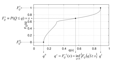
Figure 1: CDF and ICDF characteristic points.

Now that the CDF and the GIDF have been introduced, it becomes immediate to define, within the framework of multi-objective optimization, a robust optimization problem in terms of an arbitrary number of quantiles to optimize:

$$P_{Q(s_{i})}:\quad\mathop{\min}\limits_{z\in Z}q^{s_{i}}\left(z\right)=\mathop{\min}\limits_{z\in Z}\inf\left\{{q\left(z\right)\in\mathbb{R}:F_{Q}\left({q\left(z\right)}\right)\geq s_{i}}\right\}\quad i=1,\ldots,n$$ (2)

being $n$ the number of objectives chosen. The approach, then, can be further extended by introducing objectives that are arbitrary functions of quantiles.

Of course, the problem now is focused on how to satisfactorily calculate the quantiles required by the method. In this work the Empirical Cumulative Distribution Function (ECDF) is used for this purpose. The definition of ECDF, taken from [18], is reported here for the sake of completeness.

Let $X_{1},\ldots,X_{n}$ be random variables with realizations $x_{i}\in\mathbb{R}$, the empirical distribution function is an indicator function that estimates the true underlying CDF of the points in the sample. It can be defined by using the order statistics $X_{(i)}$ of $X_{i}$ as:

$$\widehat{F}_{n}(x,\omega)=\begin{cases}0&\text{if $x<x_{(1)}$;}\\ \frac{1}{n}&\text{if $x_{(1)}\leq x<x_{(2)}$, $1\leq k<2$;}\\ \frac{2}{n}&\text{if $x_{(2)}\leq x<x_{(3)}$, $2\leq k<3$;}\\ \vdots\\ \frac{i}{n}&\text{if $x_{(i)}\leq x<x_{(i+1)}$, $i\leq k<i+1$;}\\ \vdots\\ 1&\text{if $x\geq x_{(n)}$;}\end{cases}$$

where $x_{(i)}$ is the realization of the random variable $X_{(i)}$ with outcome (elementary event) $\omega\in\Omega$.

From now on, therefore, when the optimization algorithm will require the calculation of the $F_{Q}(s)$, it will used instead its estimator $\widehat{F}_{Q_{n}}(s)$, where $n$ indicates the number of samples used to estimate this ECDF.

Note that each indicator function, and hence the ECDF, is itself a random variable. This is a very delicate issue to consider. Indeed, if the EDCF is used to approximate the deterministic operator $Q(s)$, a direct residual influence of the random variables that characterize the system under investigation remains on $P_{Q(s)}$. In other words $Q(s)$ behaves as a random variable, but with the important difference that its variance tends to zero when the ECDF approximates the CDF with increasing precision. It is possible to demonstrate that the estimator $\widehat{F}_{Q_{n}}(s)$ is consistent, as it converges almost surely to $F_{Q}(s)$ as $n\rightarrow\infty$, for every value of $s$ [14]. Furthermore, for the Glivenko-Cantelli theorem [11], the convergence is also uniform over $s$. This implies that, if the ECDF is calculated with sufficient accuracy, it can be considered and treated as a deterministic operator. On the other hand, if the number of samples, or the estimation technique of the ECDF, do not allow to consider it as such, one can still correlate the variance of the ECDF with the precision of the obtained estimate. Of course, if the ECDF is estimated in a very precise way, it is possible to use for the optimization also an algorithm conceived for deterministic problems, provided that it has a certain resistance to noise. Conversely, if the ECDF is obtained from a coarse sample, its practical use is only possible with optimization algorithms specifically designed.

For the same reason, it is often convenient, especially in applications where the ECDF is defined with few samples, to use $q^{\epsilon}$ instead of $q^{0}$, with $\epsilon>0$ and small, but such that a not excessive variance of the estimate of $q^{\epsilon}$ is ensured.

4 Illustrative example

The features of the quantile curve optimization approach will be illustrated with the help of a simple example function defined as follows:

$$q(\mathbf{z},\mathbf{u})=1-\sum\limits_{i=1}^{m}{a_{i}}e^{-\beta_{i}\sum\limits_{j=1}^{n}{\left({z_{j}+u_{j}-c_{i,j}}\right)^{2}}}$$

with design parameter vector $\mathbf{z}=(z_{1},\ldots,z_{n})\in Z\subseteq\mathbb{R}^{n}$ and uncertainty vector $\mathbf{u}=(u_{1},\ldots,u_{n})\in U\subseteq\mathbb{R}^{n}$. The random variables $\mathbf{u}$ are assumed uniformly distributed with expected value $0$ and variance $1/12$. Let’s assume for the sake of compactness: $\mathbf{x}=\mathbf{z}+\mathbf{u}=(x_{1},\ldots,x_{n})=(z_{1}+u_{1},\ldots,z_{n}+u_{n})$, so the example function becomes:

$$q(\mathbf{x})=1-\sum\limits_{i=1}^{m}{a_{i}}e^{-\beta_{i}\sum\limits_{j=1}^{n}{\left({x_{j}-c_{i,j}}\right)^{2}}}$$ (3)

where the uncertain parameter $\mathbf{u}$ is incorporated in the new random variable $\mathbf{x}$ Choosing the following set of parameters:

$$\left\{{\begin{array}[]{lll}{n=1\hfill}\\ {m=4\hfill}\\ z_{1}\in\left[{0,5}\right],&\lx@intercol\hfil u_{1}\in\left[{-0.25,0.25}\right]\hfil\lx@intercol\hfill\\ a_{1}=0.9,&\beta_{1}=50.0,&{c}_{{1,1}}=1.0\hfill\\ a_{2}=0.5,&\beta_{2}=1.0,&{c}_{{2,1}}=2.5\hfill\\ a_{3}=0.8,&\beta_{3}=80.0,&{c}_{{3,1}}=4.0\hfill\\ a_{4}=0.8,&\beta_{4}=100.0&{c}_{{4,1}}=4.2\hfill\end{array}}\right.$$

the function reported in Figure 2 is obtained, where the uncertain parameter $\mathbf{u}$ is incorporated into the new random variable $\mathbf{x}$ that has expected value equal to $\mathbf{z}$ and variance equal to $1/12$. In particular, the first graph is related to the “deterministic” version of function, e.g. with $\sigma_{\mathbf{u}}=0$, while the second one reports the projection of $q(\mathbf{x})=q(\mathbf{z},\mathbf{u})$ in the plane $(\mathbf{z},q)$. The black curve corresponds to $\mathbf{u}=0$, while the contributions to $q$ due to $\mathbf{u}\neq 0$ are shown in gray and indicate the variation of the function $q$ caused by the random variable $\mathbf{u}$. Obviously, in the plane $(\mathbf{x},q)$ the effect of the random variable $\mathbf{u}$ is a simple variation of the position of the point along the curve $q$, and that is how this function will be represented in the figures below.

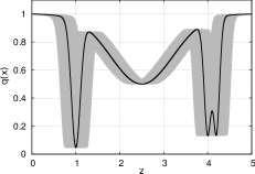
Figure 2: $q(\mathbf{z},\mathbf{u}=0)$ plot (left) and $q(\mathbf{x})$ projection in the plane $(\mathbf{z},q)$ (right).

The Empirical CDF is used to estimate the uncertainty on $q$ induced by $\mathbf{u}$:

$$\widehat{F}_{Q}(q)\approx F_{Q}(q)=P(Q\leq q)$$

Some ECDFs related to the defined $q(x)$ are reported in Figure 3. An ECDF defined in the $\left(q(x),F_{Q}(q)\right)$ plane corresponds to a function variation in the $\left(x,q(x)\right)$ plane. The correspondence between ECDF and function variation is evidenced in the figure by using the same line style.

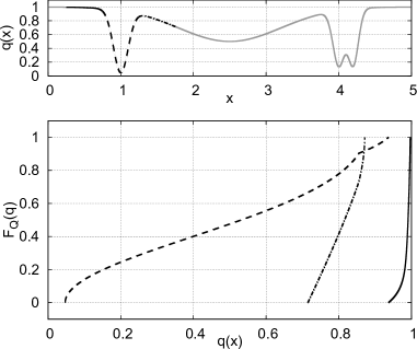
Figure 3: Some ECDFs related to $q(x)$.

Let’s now consider the following two-objective problem:

$$\mathop{\min}\limits_{x}\left({q^{\epsilon},q^{1-\epsilon}}\right)$$ (4)

where the use of a small $\epsilon$ value is introduced to account for the approximation introduced by the ECDF estimator. Figure 4 reports the results obtained with problem formulation (4). The extreme of the Pareto front related to the best $\mathrm{Obj}_{1}$, namely $q^{\epsilon}$, is representative of the best possible optimum, without regard to the variance. The front extreme related to the best $\mathrm{Obj}_{2}$ gives, instead the most robust solution, e.g. the one that that has the least variance. Finally, the solution located in the middle of the front represents a compromise between best absolute performance and smallest variance.

Figure 5 reports, as a dot-dashed line, the Pareto front obtained solving the problem

$$\mathop{\min}\limits_{x}\left({q^{0.25},q^{1-\epsilon}}\right)$$ (5)

Here the solutions with higher variance are no longer present on the Pareto front, and this is often a desirable behavior in a robust design problem. Among the solutions which are on the left side of the front, the one with lowest $\mathrm{Obj}_{2}$ should be selected. Indeed, the significant worsening observed in the second objective is not compensated by an adequate improvement of the first one.

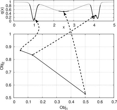
Figure 4: Pareto front of problem formulation 1.

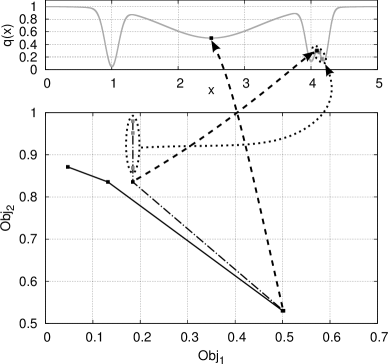
Figure 5: Pareto front of problem formulation 2.

Figure 6: ECDF estimated using just 20 uniform samples.

Finally, it is worth to see what should be expected when the estimate of the CDF is very coarse. Consider, in this regard, a ECDF calculated with only 20 samples distributed uniformly (see Figure 6). Here, both the problem (4) and problem (5) do not allow to discern between the solution with maximum variance and the one giving an intermediate compromise. If, instead, the following problem is solved

$$\mathop{\min}\limits_{X}\left({q^{0.45},q^{1-\epsilon}}\right)$$ (6)

it is possible to exclude the solution with maximum variance from the Pareto front, as can be observed by analyzing Figure 7. Thus, this approach is definitely worth to be tested when a sufficiently precise estimate of the CDF is not available.

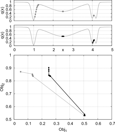
Figure 7: Comparisons of Pareto fronts and related results of problems $\left({q^{\epsilon},q^{1}}\right)$, dotted curve, and $\left({q^{0.45},q^{1}}\right)$, solid curve.

5 A benchmark function with variable number of design parameters

The function reported in Table 1, taken from [15], is used as a benchmark to test the GIDF based approach to robust optimization. With respect to the function reported in the reference, the following changes have been introduced: the ranges of design and uncertain parameters have been changed as reported in table, and a multiplicative factor equal to $1/n$ has been introduced to make easier the result comparison when the dimension of the parameter space changes. The random variables $\mathbf{u}$ have a uniform distribution function. Table 2 reports the solutions to the optimization problems

$$\min\limits_{\mathbf{d}\in D,\mathbf{u}\in U}f(\mathbf{d},\mathbf{u})$$

$$\min\limits_{\mathbf{d}\in D}\max\limits_{\mathbf{u}\in U}f(\mathbf{d},\mathbf{u})$$

over the cartesian product of $D$ and $U$. The first problem represents the best possible solution obtainable if the $\mathbf{u}$ are considered as design parameters varying in $U$. The second one, instead, minimizes the maximum possible loss or, alternatively, maximizes the minimum gain, according to the framework of decision theory [7]. These solutions have been obtained analytically and verified by exhaustive search for $n=1$. It is worth to note that these particular optimal solutions are the same whatever is the dimension of the search space.

The optimization algorithm used here is a simple multi-objective genetic algorithm not specially conceived for optimization under uncertainty. The algorithm is based on the Pareto dominance concept [2] and on local random walk selection [10, 16]. Crossover operator is the classical one-point crossover which operates at bit level, while mutation operator works at the level of the design vector parameters (which are real numbers). A parameter, called mutation rate controls the operator activation probability for each variable vector element, while a further parameter, called strength, is the maximum relative value the uniform word mutation. The word mutation value is given by $\mathrm{strength}\cdot(r-0.5)(u-l)$ with $r\in[0,1]$ uniform random number, $u$ upper variable bound and $l$ lower variable bound. An elitist strategy was adopted in the optimization runs. It consists in replacing 20% of the population calculated at each generation with elements taken at random from the current Pareto front. Obviously, the elements of the population are used to update the current Pareto front before the replacement, in order to avoid losing non-dominated population elements.

The multi-objective runs were performed using 100% crossover activation probability and word mutation with mutation rate equal to 50% and strength equal to 0.06. The initial population was obtained using the quasi-random low-discrepancy Sobol sequence [1]. The ECDF used to estimate the CDF was obtained with 2500 Montecarlo samples in all runs. The population size was set to 4000 elements for all runs, while the number of generations was set to $10$ for $n=1$, $200$ for $n=2$ and $1000$ for $n=6$. The problem solved was $\min\limits_{\mathbf{z}\in Z}\left({q^{\epsilon},q^{1-\epsilon}}\right)$.

Table 1: Benchmark functions table.

ID	Function	Ranges	Dimension
MV4	$f=\frac{1}{n}\sum\limits_{i=1}^{n}{\left({2\pi-u_{i}}\right)\cos\left({u_{i}-d_{i}}\right)}$	$\mathbf{u}\in\left[{0,3}\right]^{n},\mathbf{d}\in\left[{0,2\pi}\right]^{n}$	1, 2 and 6

Table 2: Benchmark functions table results.

ID	$\min\limits_{\mathbf{d}\in D,\mathbf{u}\in U}f(\mathbf{d},\mathbf{u})$			$\min\limits_{\mathbf{d}\in D}\max\limits_{\mathbf{u}\in U}f(\mathbf{d},\mathbf{u})$
	$\qquad\mathbf{d}\qquad$	$\qquad\mathbf{u}\qquad$	$f$	$\qquad\mathbf{d}\qquad$	$\qquad\mathbf{u}\qquad$	$f$
MV4	$[3.1416]^{n}$	$[0]^{n}$	$-6.283185\ldots$	$[4.6638]^{n}$	$[0]^{n}$	$-0.305173\ldots$

Figure 8 reports the Pareto fronts and the deterministic $\min$ and $\min\max$ solutions obtained for the MV4 test case at different values of the design space size $n$. It can be easily observed that, in the case $n=1$, the extremes of the front are practically coincident with the deterministic solutions, while, in the case $n=2$, the solution of the Pareto front which minimizes the second objective $(q^{1-\epsilon})$ underestimates the $\min\max$ solution. The trend is even more evident in the case $n=6$, where, indeed, also the extreme of the front that minimizes the first goal $(q^{\epsilon})$ overestimates the value obtained from the $\min$ problem. This can be explained by the fact that the two deterministic solutions are located in correspondence with the extremes of variation of the random variables of the problem. Therefore, as the number of random variables increases, in accordance with the central limit theorem [12], it becomes less likely that all random variables are located in correspondence of one of their limits of variation. Anyway, as illustrated in Figure 9, when the Pareto front obtained with the sample size $m$ equal to 2500 is re-evaluated with a larger Montecarlo sample, the obtained curve is a quite acceptable approximation of the Pareto front obtained with $m=100000$.

It should be noted that, for the problem at hand, it is possible to determine a close approximation of the exact Pareto front for any value of $n$, once a good approximation is known (or the exact Pareto front) the for $n=1$ case. Note, in this regard, that if $f(\mathbf{x})$, with $n\neq 1$ and $\mathbf{x}=\left(x_{1},\ldots,x_{n}\right)$, is non-dominated, then so are all its components $f_{1}(x_{1}),\ldots,f_{1}(x_{n})$. So the elements belonging to the Pareto front with $n\neq 1$ may be constructed by adding elements belonging to the front with $n=1$. However, not all these elements belong to the Pareto front (with $n\neq 1$), for which it will be necessary to extract the non-dominated elements among all those obtained in this way. Figure 10 reports the Pareto fronts at $n=2$ and $n=6$ obtained with this technique.

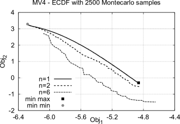
Figure 8: Pareto fronts and deterministic $\min$ and $\min\max$ solutions for the MV4 test case.

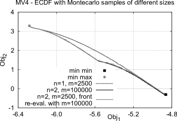
Figure 9: Pareto fronts for the MV4 test case obtained with different sizes for Montecarlo sampling.

Figure 10: Pareto fronts for the MV4 test case obtained with the exact method.

Figure 11: Optimal ECDF curves for the MV4 with $n=1$.

Figure 12: Optimal ECDF curves for the MV4 with $n=6$.

Figures 11 and 12 show the ECDF corresponding to the extremes of the Pareto front, respectively for the cases $n=1$ and $n=6$. It is noted, again in accordance with the central limit theorem, that, in the case $n=6$, the ECDF curves are very close to those related to a Gaussian distribution.

6 Evaluating and improving the quantile estimation

The example in the previous section shows very clearly that the results of the proposed method may depend in an essential way on the quality of estimation of quantiles that is obtained through the ECDF. This leads in a natural way to deal with two issues: how to evaluate the quality of the estimation of the quantiles used in the multi-objective optimization problem, and how to possibly get a better quantile estimate with a given computational effort. Related to these two points, however, there are other problems too: it is possible to conceive an algorithm that can account for the error in the estimation of the quantiles? is it possible to find estimators of ECDF that give the required accuracy in the computation of the quantiles of interest for the optimization problem?

The approach here proposed for assessing the quality of the estimate of the quantile is based on the bootstrap method introduced by Efron in 1977 [4, 3].

This method represents a major step forward in the statistical practice because it allows to accurately assess the variability of any statistical estimator without making any assumption about the type of distribution function involved. Suppose that a statistic $T\left(x_{1},x_{2},\ldots,x_{n}\right)$ is given, evaluated on a set of data $x_{1},x_{2},\ldots,x_{n}$ belonging to an assigned space $X$. The bootstrap essentially consists in repeatedly recalculate the statistic $T$ employing a tuple of new samples $x^{*}_{1},x^{*}_{2},\ldots,x^{*}_{n}$ obtained by selecting them from the collection $\left\{x_{1},x_{2},\ldots,x_{n}\right\}$ with replacement. The repeated calculation of $T\left(x^{*}_{1},x^{*}_{2},\ldots,x^{*}_{n}\right)$ gives a set of values that gives a good indication of the distribution of $T$.

Therefore, to calculate the accuracy of a generic quantile $q^{s}$, obtained by the estimator $\widehat{F}_{Q_{n}}(s)$, the bootstrap procedure can be applied to the samples that define the estimator. This allows to calculate the corresponding distribution of $q^{s}$ for a fixed value of $s$.

Figure 13 reports the ECDF related to the solution labeled as “MOST ROBUST” in Figure 12. The bootstrap was applied to this ECDF repeating the sampling process 2000 times. The area in gray color represents the superposition of all the curves obtained in this way. From the bootstrap data it is then possible to evaluate the accuracy of a given quantile estimate. Figure 14 reports the ECDF of three different quantiles (namely $q^{0.001},q^{0.500},q^{0.999}$) obtained from the “MOST ROBUST” solution to MV4. According to [3], an accuracy measure for $q^{s}$ can be obtained considering the central 68% of bootstrap samples. These values lay between an interval $[q^{s}_{\ell},q^{s}_{u}]$ centered on the observed value $q^{s}$. Half the length of this interval gives a measure of the accuracy for the observed value that corresponds to the traditional concept of “standard error”. Here this value vill be indicated with $\widehat{SE}$ to distinguish it from the true standard error $SE$.

Table 3 reports the computed accuracy values for the considered quantiles for the above cited “MOST ROBUST” solution obtained from an ECDF with 2500 Montecarlo samples. The fourh column reports, finally, the maximum estimated error $\widehat{ME}$.

Table 3: Quantile estimates and related accuracy for MV4 “MOST ROBUST” solution with $n=6$.

$s$	$q^{s}$	$\widehat{SE}$	$\widehat{ME}$
$0.001000$	$-4.630433$	$\pm 0.090423$	$\pm 0.117169$
$0.500000$	$-3.230388$	$\pm 0.018834$	$\pm 0.054983$
$0.999000$	$-1.425868$	$\pm 0.013192$	$\pm 0.136330$

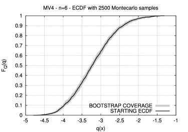
Figure 13: ECDF corresponding to the most robust solution and related bootstrap coverage.

Figure 14: Cumulative distributon curves accounting for the uncertainty of quantiles evaluation obtained with the bootstrap method.

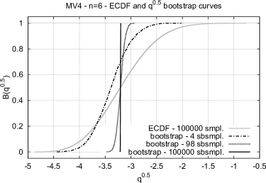
Figure 15: Bootstrap curves for $q^{0.5}$ and high resolution ECDF for the MV4 “MOST ROBUST” solution with $n=6$.

Figure 16: Standard and maximum error for $q^{0.5}$ as a function of the number of samples for the MV4 “MOST ROBUST” solution with $n=6$.

The bootstrap is useful for characterizing the standard error of a given sample used to construct the ECDF, but it is even more important to try to describe how the error varies depending on the number of elements of the sample. To obtain this estimate, a variant of the bootstrap process is proposed here in which the starting point is a ECDF calculated with many Montecarlo samples, so as to get as close as possible to the true CDF. From these data, the bootstrap is applied by drawing a number of samples smaller than the size of the original sampling. Note that if the number of samples of the bootstrap is equal to one, we obtain the starting ECDF. As can be seen from Figure 15, the bootstrap curves tend to widen when the number of used samples decreases. From these curves it is possible to derive the estimates of standard and maximum errors with the same procedure used to construct Table 3. Figure 16 shows, on a logarithmic scale, $\widehat{SE}$ and $\widehat{ME}$ as a function of the number of samples used to bootstrap $q^{0.5}$. The important thing to note is that, already with a number of elements that ranges from 10 to 100, values of $\widehat{SE}$ and $\widehat{ME}$ are got that an ad hoc designed optimization algorithm could handle.

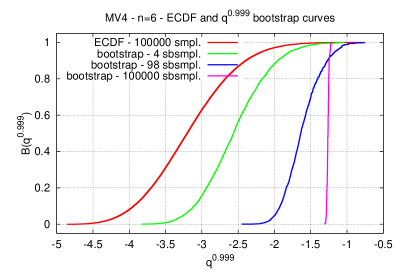
Figure 17: Bootstrap curves for $q^{0.999}$ and high resolution ECDF for the MV4 “MOST ROBUST” solution with $n=6$.

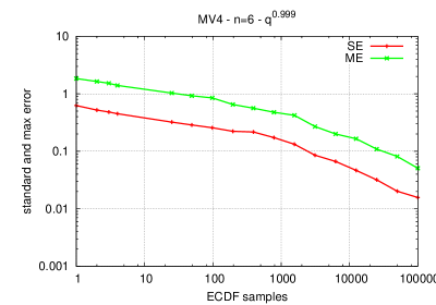
Figure 18: Standard and maximum error for $q^{0.999}$ as a function of the number of samples for the MV4 “MOST ROBUST” solution with $n=6$.

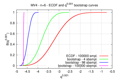
Figure 19: Bootstrap curves for $q^{0.001}$ and high resolution ECDF for the MV4 “MOST ROBUST” solution with $n=6$.

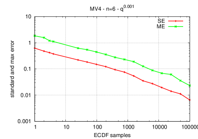
Figure 20: Standard and maximum error for $q^{0.001}$ as a function of the number of samples for the MV4 “MOST ROBUST” solution with $n=6$.

The analysis of Figures 17–18, related to $q^{0.999}$, and Figures 19–20, related to $q^{0.001}$, confirms the same trends previously detected, but $\widehat{SE}$ and $\widehat{ME}$ errors remain higher, confirming the fact that it is more difficult to describe the statistical tails compared to median values.

7 Many objectives formulation

The multi-objective formulation can be interpreted in a way that might be advantageous in some cases. Suppose indeed to consider a very large number, even infinite, of quantiles in the definition of the optimization problem 2. This results in the problem that optimization follows:

$$\left\{{\begin{array}[]{*{20}c}{\mathop{\min}\limits_{X}q^{s_{i}}=F_{Q}^{-1}\left({s_{i}}\right)\hfill}&\hfill{}\hfil\\ {s_{i}=i/n\hfill}&{i=1,n\hfill}\\ \end{array}}\right.$$ (7)

with $s\in[0,1]$ equally spaced probability thresholds. The aim of this approach is to control and optimize the entire shape of the CDF. This point can be illustrated with the help of an example. Consider again the example described in Section 4. The CDF curves related to all the possible elements of the set of definition of the function $q$, numbered as (3), are shown in light gray in Figure 21. In the same figure, the CDF curves of the non dominated elements are reported in dark gray and, finally, the envelope of the non dominated CDF curves is reported in black. It represents an “IDEAL” CDF for the problem at hand, that is, a limit curve that outperforms any true CDF and that can be adopted as a target in a template optimization process as the one presented in [8].

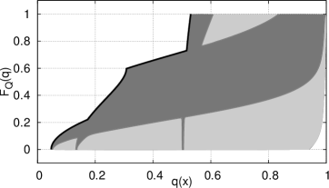
Figure 21: Non-dominated envelop of all CDF curves.

8 Solving an evidence theory optimization problem

The same numerical machinery used for the GIDF can be immediately adopted, with the addition of a few supplementary steps, to the approximate estimation of the “belief” and “plausibility” curves introduced in the “Evidence Theory” when this theory is applied to solve robust optimization problems. Indeed, belief, plausibility and GIDF computations start from a sample of the uncertainty variable parameter space, followed by the computation of the ECDF, to the heart of which there is a sorting operation. Similarly to the GIDF case, the obtainable level of approximation for belief and plausibility curve computation depends strongly on the quality and resolution of the ECDF and is, hence, controllable.

The definition of the belief and plausibility is here biefly summarized for the sake of clarity and completeness. For each uncertain variable, the evidence theory assigns, at given intervals, which can also be partially overlapping, values called “Basic Probability Assignment” (BPA), which express the degree of confidence that the experts have on that parameter. The BPA represents, in the framework of evidence theory, the element that controls the propagation of information. So, the BPA allows to characterize each realization of a given random variable $u$ in a way similar to the probability distribution function. The conceptual difference is that here we are not dealing with true probability distribution functions, but with probability bounds defined by experts. The BPA has to follow some simple rules that are reported in the followings. Let $U$ be the set ov variation of an uncertain parameter $u$, e.g. the interval $[-3,5]$ in the example of Table 4, and let $\Xi=\{E_{1},\ldots,E_{n}\}$ a set of subsets of $U$ (e.g. $\bigcup_{i=1}^{n}E_{i}\subseteq U$). A real, non-negative value $m$, namely the basic probability, can be assigned to each element $E_{i}\in\Xi$ according to the following rules:

$$\left\{\begin{array}[]{ll}m(E_{i})\geq 0&\forall E_{i}\in\Xi\\ m(\emptyset)=o\\ \displaystyle\sum_{E_{i}\in\Xi}m(E_{i})=1\end{array}\right.$$ (8)

The subset $\Phi=\{FE_{1},\ldots,FE_{m}\}\subseteq\Xi$ of the elements with non-zero value of $m$ is called the focal element set. The extension to more than one uncertain parameter is easily obtained with the help of Cartesian product. The assignment of a basic probability value set to each uncertain parameter allows the computation of belief and plausibility values for logical propositions involving these parameters. Given a proposition $\alpha$, true in a subset $A$ of $U$, the belief and plausibility values are defined as:

$$\begin{array}[]{rccl}\mathrm{Bel}(\alpha)&=&\displaystyle\sum_{FE\subseteq A}&m(FE)\\ \mathrm{Pl}(\alpha)&=&\displaystyle\sum_{FE\cap A\neq\emptyset}&m(FE)\end{array}$$ (9)

sub-interval	BPA
$[-5,-4]$	0.1
$[-3,0]$	0.25
$[1,3]$	0.65

Table 4: BPA structure for an uncertain variable $u$ defined in $[-5,3]$ interval.

In the application of evidence theory to robust optimization, the proposition $\alpha$ is often defined as a parametric inequality involving a function $f(u,d)$ of uncertain parameters $u\in U$ and design variables $d\in D$, and a threshold value $\nu$:

$$f(u,d)\leq\nu$$ (10)

In these cases a strong connection is evident with the cumulative distribution function, that will be used to obtain an approximate evaluation of belief and plausibility curves. The steps to follow are enumerated in the following subsections

Affine mapping of the uncertain parameter space

For each uncertain variable, the evidence theory assigns, at given subsets, which can also be partially overlapping, the BPA values. To the purpose of numerical computation, these BPA focus on assigned regions of the design space that can be also non-connected. A sample BPA definition for a given uncertain parameter is reported in table 4. In order to restore the connectivity of the design space, and to make easier the numerical computation, an affine mapping is applied to the design space that is remapped in the unity cube. In the present method, the affine mapping is replaced by a CDF built for each uncertain input variable. This CDF assigns uniform selection probabilities to each of the BPA intervals selected by the experts for that variable. Figure 22 illustrates the mapping of the BPA defined in Table 4 into the CDF that replaces the affine mapping in the current approach.

Figure 22: Mapping of the BPA into a CDF.

Calculation of belief and plausibility using the ECDF

As it appears evident from formula 9, the calculation of $\mathrm{Bel}(f(u,d)\leq\nu)$, for a given $d$, requires, for each focal element $FE\in A$, the computation of the maximum value of $f(u,d)$:

$$\max_{u\in FE}f(u,d)$$ (11)

Similarly, the computation of the plausibility, $\mathrm{Pl}(f(u,d)\leq\nu)$, requires the determination of the set of minimum values of $f(u,d)$:

$$\min_{u\in FE}f(u,d)$$ (12)

If a ECDF of $f(u,d)$ with $n$ samples is available, along with a mapping that associates each point of the ECDF with its focal element $FE$, then it is possible to estimate the belief curve. More formally, if $f_{i}$ is the $i$-th point of the ECDF, the mapping function can be written as:

$$p_{i}:f_{i}\in\mathrm{ECDF}\longmapsto\mathrm{FE}_{i}\in U$$ (13)

and the related BPA value is indicated with $b_{i}$. This is the most critical point. The accuracy of this mapping is the key to obtain an accurate estimation!

For a given value $\nu^{\star}$ of the proposition threshold, the belief value can be obtained considering the subset of the ECDF samples defined by

$$M_{\nu^{\star}}=\left\{f_{i}:f_{i}>\nu^{\star},f_{i}\in\mathrm{ECDF}\right\}$$ (14)

Considering that the ECDF is, by definition, sorted with respect the $f_{i}$ values, it is convenient to define an index function $q=q(M_{\nu^{\star}})$ that maps the smaller element of $M_{\nu^{\star}}$ to the corresponding element position in the ECDF. The estimation of the belief is thus given by:

$$\hat{B}_{\nu^{\star}}=\widehat{\mathrm{Bel}}(f(u,d)\leq\nu^{\star})=1-\sum_{j=q}^{n}s_{j}$$ (15)

where

$$s_{j}=\left\{\begin{array}[]{cl}b_{j}&\textrm{if}\;p_{j}\neq p_{\nu^{\star}}\;\textrm{and}\;p_{j}\neq p_{k},\forall k=q,j-1\\ 0&\textrm{otherwise.}\end{array}\right.$$ (16)

The calculation of plausibility is very similar, but with the important difference that the BPA of the $FE_{\nu^{\star}}$ must be considered in the related formulas. Therefore let:

$$N_{\nu^{\star}}=\left\{f_{i}:f_{i}\geq\nu^{\star},f_{i}\in\mathrm{ECDF}\right\}$$ (17)

and $r=q(N_{\nu^{\star}})$. So the plausibility estimation is given by

$$\hat{P}_{\nu^{\star}}=\widehat{\mathrm{Pl}}(f(u,d)\leq\nu^{\star})=1-\sum_{j=r}^{n}t_{j}$$ (18)

where

$$t_{j}=\left\{\begin{array}[]{cl}b_{j}&\textrm{if}\;p_{j}\neq p_{k},\forall k=r,j-1\\ 0&\textrm{otherwise.}\end{array}\right.$$ (19)

The approximated belief and plausibility curves thus obtained can be immediately used in the optimization process.

Listing 1: C code for belief and plausibility estimation.

⬇

#include <stdlib.h>

#include <stdio.h>

#include <math.h>

#include <string.h>

/*

* Extended ECDF structure

*/

typedef struct {

double f; /* Function value */

char hash[100]; /* Focal point id label */

int hash_min; /* In a vector of ecdf_t elements sorted with respect to f hash_min is set to 1

for the first focal point with the same hash label encountered */

int hash_max; /* In a vector of ecdf_t elements sorted with respect to f hash_max is set to 1

for the last focal point with the same hash label encountered */

double bpa; /* Basic probability assignment for the focal element to which f belongs */

double belief;

double plausibility;

} ecdf_t;

double MV1(double *d, double *u, int n);

double MV2(double *d, double *u, int n);

double MV8(double *d, double *u, int n);

void belief_and_plausibility_estimator(double (*f)(double*, double*, int),

void (*affmap)(int, double*, double*), char (*feid)(double),

double (*bpa_component)(char), double *d, double ul, double uu, int n,

int m, ecdf_t *Ecdf);

void uranvec(double *x, int n, double xl, double xu) {

int i;

for (i = 0; i < n; i++) {

x[i] = xl + (xu - xl) * drand48();

}

}

/*

* Begin of Problem Dependent Data

*/

double affine_mapping_MV1_comp(double x) {

/* Affine mapping for the MV1 function variable vector components */

double y;

if (x >= 0 && x <= 0.1)

y = -5 + (-4 + 5) * x / 0.1;

else if (x > 0.1 && x <= 0.1 + 0.25)

y = -3 + (0 + 3) * (x - 0.1) / 0.25;

else

y = 1 + (3 - 1) * (x - 0.35) / 0.65;

return y;

}

void affine_mapping_MV1(int n, double *x, double *mx) {

int i;

for (i = 0; i < n; i++)

mx[i] = affine_mapping_MV1_comp(x[i]);

}

char focal_element_id_MV1(double x) {

/*

* Computes the focal element id related to a single vector variable component

* (after the affine transformation) for the MV1 function.

*/

char y;

if (x >= -5 && x <= -4)

y = ’0’;

else if (x > -3 && x <= 0)

y = ’1’;

else if (x > 1 && x <= 3)

y = ’2’;

else

exit(0); /* ERROR: Out of considered intervals. */

return y;

}

double bpa_component_MV1(char x) {

/*

* Basic probability assignment for a single vector variable component

* of the MV1 function.

*/

int iu;

double bpa_c = 0;

iu = x - ’0’;

switch (iu) {

case 0:

bpa_c = 0.10;

break;

case 1:

bpa_c = 0.25;

break;

case 2:

bpa_c = 0.65;

break;

}

return bpa_c;

}

double MV1(double *d, double *u, int n) {

/*

* $\sum_{i=1}^{n} d_i u_i^2, d\in[1,5]^n, u\in[-5,3]^n

*/

double objective;

int i, j;

objective = 0;

for (j = 1; j <= n; j++) {

i = j - 1;

objective += d[i] * (u[i] * u[i]);

}

return objective;

}

double MV2(double *d, double *u, int n) {

/*

* $\sum_{i=1}^{n}(u_i-d_i)^2, d\in[1,5]^n, u\in[-5,3]^n

*/

double objective;

int i, j;

objective = 0;

for (j = 1; j <= n; j++) {

i = j - 1;

objective += (u[i] - d[i]) * (u[i] - d[i]);

}

return objective;

}

double MV8(double *d, double *u, int n) {

/*

* $\sum_{i=1}^{n}(2\pi-u_i)\cos(u_i-d_i)^2, d\in[0,3]^n, u\in[0,2\pi]^n

*/

double objective;

int i, j;

objective = 0;

for (j = 1; j <= n; j++) {

i = j - 1;

objective += (2 * M_PI - u[i]) * cos(u[i] - d[i]);

}

return objective / n;

}

/*

* End of Problem Dependent Data

*/

static int dcomp_ecdf_t(ecdf_t *a, ecdf_t *b) {

if (a->f < b->f)

return -1;

if (a->f > b->f)

return +1;

return 0;

}

void belief_and_plausibility_estimator(double (*f)(double*, double*, int),

void (*affmap)(int, double*, double*), char (*feid)(double),

double (*bpa_component)(char), double *d, double ul, double uu, int n,

int m, ecdf_t *Ecdf) {

double u[n], amu[n];

int i, j;

for (i = 0; i < m; i++) {

uranvec(u, n, ul, uu);

affmap(n, u, amu);

Ecdf[i].f = f(d, amu, n);

Ecdf[i].bpa = 1;

for (j = 0; j < n; j++) {

Ecdf[i].hash[j] = feid(amu[j]);

Ecdf[i].bpa *= bpa_component(Ecdf[i].hash[j]);

}

Ecdf[i].hash[n] = 0;

Ecdf[i].hash_min = 1;

Ecdf[i].hash_max = 1;

}

qsort(Ecdf, m, sizeof(ecdf_t),

(int (*)(const void *, const void *)) dcomp_ecdf_t);

for (i = m - 1; i >= 0; i–) {

if (Ecdf[i].hash_max == 1)

for (j = i - 1; j >= 0; j–) {

if (strcmp(Ecdf[i].hash, Ecdf[j].hash) == 0)

Ecdf[j].hash_max = 0;

}

}

for (i = 0; i < m; i++) {

if (Ecdf[i].hash_min == 1)

for (j = i + 1; j < m; j++) {

if (strcmp(Ecdf[i].hash, Ecdf[j].hash) == 0)

Ecdf[j].hash_min = 0;

}

}

for (i = 0; i < m; i++) {

Ecdf[i].belief = 1;

for (j = i + 1; j < m; j++) {

if (Ecdf[j].hash_max == 1)

Ecdf[i].belief -= Ecdf[j].bpa;

}

}

for (i = 0; i < m; i++) {

Ecdf[i].plausibility = 1;

for (j = i + 1; j < m; j++) {

if (Ecdf[j].hash_min == 1)

Ecdf[i].plausibility -= Ecdf[j].bpa;

}

}

}

#define NUMBER_OF_OUTPUT_VARIABLES 10000

#define VECTOR_VARIABLE_SIZE 1

int main() {

/*

* Compute belief and plausibility

*/

ecdf_t Ecdf[NUMBER_OF_OUTPUT_VARIABLES];

double r[VECTOR_VARIABLE_SIZE];

int n = VECTOR_VARIABLE_SIZE, i, m = NUMBER_OF_OUTPUT_VARIABLES;

FILE *BEL, *PLA;

srand48(1234);

for (i = 0; i < n; i++)

r[i] = 1;

belief_and_plausibility_estimator(MV1, affine_mapping_MV1,

focal_element_id_MV1, bpa_component_MV1, r, 0, 1, n,

NUMBER_OF_OUTPUT_VARIABLES, Ecdf);

BEL = fopen(”belief.dat”, ”w”);

for (i = 0; i < m; i++) {

fprintf(BEL, ”HASH␣%s␣%d␣%d␣%lf␣%lf␣%lf\n”, Ecdf[i].hash,

Ecdf[i].hash_min, Ecdf[i].hash_max, Ecdf[i].f, Ecdf[i].bpa,

Ecdf[i].belief);

}

fclose(BEL);

PLA = fopen(”plausibility.dat”, ”w”);

for (i = 0; i < m; i++) {

fprintf(PLA, ”HASH␣%s␣%d␣%d␣%lf␣%lf␣%lf\n”, Ecdf[i].hash,

Ecdf[i].hash_min, Ecdf[i].hash_max, Ecdf[i].f, Ecdf[i].bpa,

Ecdf[i].plausibility);

}

fclose(PLA);

return 0;

}

8.1 A simple example

The MV1 test function (see ref. [15]) is used to illustrate the ECDF based belief and plausibility estimation method:

$$f=\sum_{i=1}^{n}d_{i}u_{i}^{2}$$ (20)

with design parameter vector $\mathbf{d}\in[1,5]^{n}$ and uncertain parameter vector $\mathbf{u}\in[-5,3]^{n}$. The BPA is the one already reported in Table 4, and the computations have been made with the design parameter vector assigned to $\mathbf{d}=[1]^{n}$.

The curves of belief and plausibility for the test function MV1, calculated using the method above, are shown in Figures 23, 24 and 25. These figures show also the exact belief and plausibility curves for the given test case in order to allow the evaluation of the actual potential of the method. What is clear is that the obtained estimate, while acceptable, is not conservative, and therefore some caution is required in the use of the results.

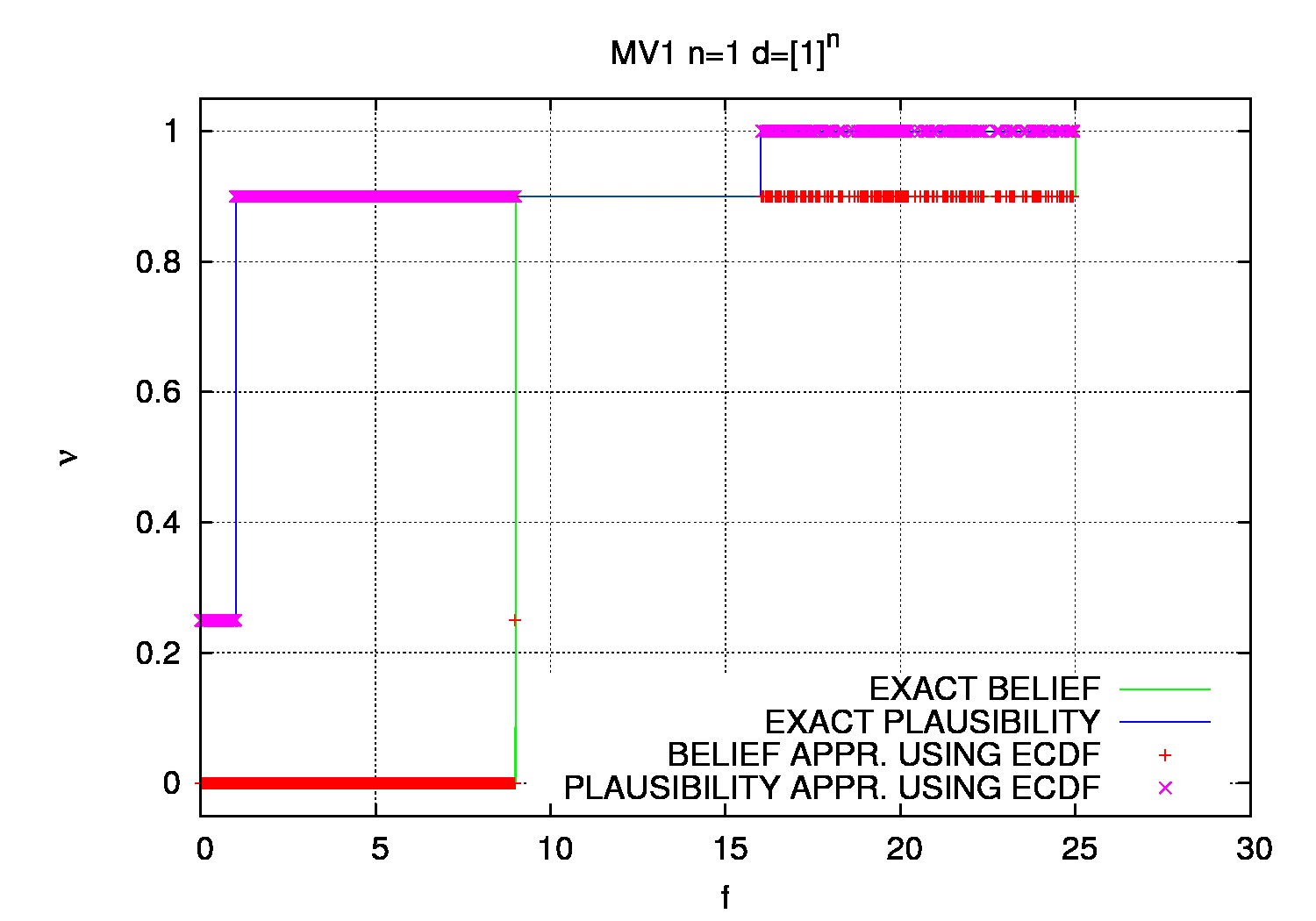
Figure 23: MV1 test function with design and uncertain parameter space size equal to 1.

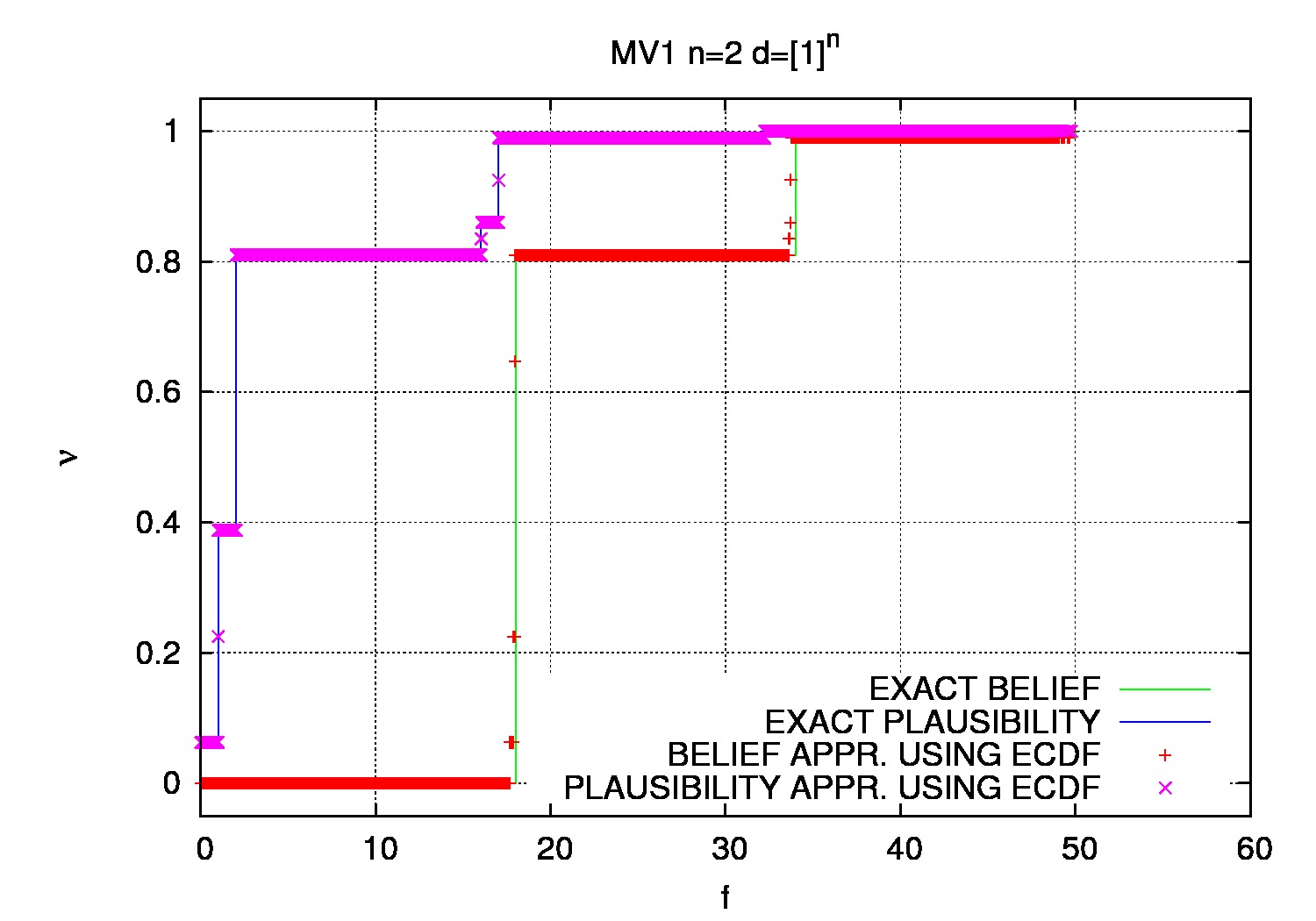
Figure 24: MV1 test function with design and uncertain parameter space size equal to 2.

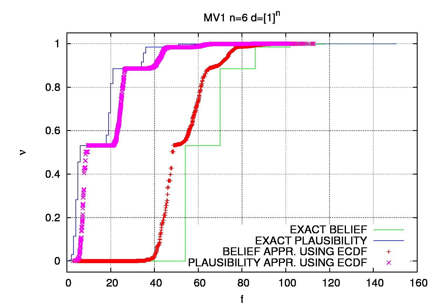
Figure 25: MV1 test function with design and uncertain parameter space size equal to 6.

9 Conclusions

An alternative approach to the optimization under uncertainty has been introduced with the help some simple test cases. The first one was a very simple and well behaved test function that had the only purpose of illustrating the main feature of the quantile based optimization method. A further example function with variable number of uncertain and design parameters was then introduced to highlight the critical points of the method related to the problem dimension. In particular, it has been discussed and illustrated how the problem features change when the number of random variables involved increases. Work is under way to better characterize the error introduced by the ECDF estimator as a function of the number of random parameters.

The algorithm used for optimization is a classical genetic algorithm, but, to further improve the proposed procedure, an optimization algorithm capable of accounting for the errors in the estimation of the CDF has to be conceived. This is a very important topic and it will be subject of next research work. In particular, to reduce the curse of dimensionality the effect of different sampling methodologies, like stochastic collocation, on the estimation of the ECDF will be considered in future works. Indeed the possibility to use the error on the ECDF estimator to properly refine the probability space using adaptive uncertainty quantification algorithms will be explored.

It is, finally, very important to to relate the results of this new optimization approach to those deriving from the application of more conventional methods, and to introduce a quantitative approach when different algorithms for robust optimization are compared.

10 Appendix

References

- [1] Bratley, P., Fox, B.L.: Algorithm 659: Implementing sobol’s quasirandom sequence generator. ACM Trans. Math. Softw. 14(1), 88–100 (1988). DOI 10.1145/42288.214372. URL http://doi.acm.org/10.1145/42288.214372
- [2] Deb, K.: Multi-Objective Optimization Using Evolutionary Algorithms. John Wiley & Sons, Inc., New York, NY, USA (2001). ISBN:047187339X
- [3] Diaconis, P., Efron, B.: Computer intensive methods in statistics. Tech. Rep. 83, Division Of Biostatistics, Stanford University (1983)
- [4] Efron, B.: Bootstrap methods: Another look at the jackknife. Annals of Statistics 7(1), 1–26 (1979). URL http://projecteuclid.org/euclid.aos/1176344552
- [5] Filomeno Coelho, R., Bouillard, P.: Multi-objective reliability-based optimization with stochastic metamodels. Evolutionary Computation 19(4), 525–560 (2011)
- [6] Hughes, E.: Evolutionary multi-objective ranking with uncertainty and noise. In: Evolutionary multi-criterion optimization, pp. 329–343. Springer (2001)
- [7] von Neumann, J., Morgenstern, O.: Theory Of Games And Economic Behavior. Princeton University Press, Princeton (1953)
- [8] Petrone, G., Iaccarino, G., Quagliarella, D.: Robustness criteria in optimization under uncertainty. In: C. Poloni, D. Quagliarella, J. Periaux, N. Gauger, K. Giannakoglou (eds.) EUROGEN 2011 PROCEEDINGS — Evolutionary and Deterministic Methods for Design, Optimization and Control with Applications to Industrial and Societal Problems, ECCOMAS Thematic Conference, pp. 244–252. ECCOMAS, CIRA, Capua, Italy (2011)
- [9] Poloni, C., Padovan, Parussini, L., Pieri, S., Pediroda, V.: Robust design of aircraft components: a multi-objective optimization problem. In: Von Karman Institute for Fluid Dynamics, Lecture Series (2004). Von Karman Institute for Fluid Dynamics, Lecture Series 2004-07
- [10] Quagliarella, D., Vicini, A.: GAs for aerodynamic shape design II: multiobjective optimization and multi-criteria design. In: Lecture Series 2000-07, Genetic Algorithms for Optimisation in Aeronautics and Turbomachinery. Von Karman Institute, Belgium (2000)
- [11] Serfling, R.J.: Approximation Theorems of Mathematical Statistics. John Wiley & Sons, Inc. (2008). DOI 10.1002/9780470316481. URL http://dx.doi.org/10.1002/9780470316481.indsub
- [12] Sobol, I.M.: A Primer for the Monte Carlo Method. CRC Press (1994)
- [13] Teich, J.: Pareto-front exploration with uncertain objectives. In: Evolutionary multi-criterion optimization, pp. 314–328. Springer (2001)
- [14] van der Vaart, A.W.: Asymptotic Statistics. Cambridge University Press (1998). URL http://dx.doi.org/10.1017/CBO9780511802256
- [15] Vasile, M., Minisci, E.: An evolutionary approach to evidence-based multi-disciplinary robust design optimisation. In: C. Poloni, D. Quagliarella, J. Periaux, N. Gauger, K. Giannakoglou (eds.) EUROGEN 2011 PROCEEDINGS — Evolutionary and Deterministic Methods for Design, Optimization and Control with Applications to Industrial and Societal Problems, ECCOMAS Thematic Conference. ECCOMAS, CIRA, Capua, Italy (2011)
- [16] Vicini, A., Quagliarella, D.: Inverse and direct airfoil design using a multiobjective genetic algorithm. AIAA Journal 35(9), 1499–1505 (1997)
- [17] Wikipedia: Cumulative distribution function. URL http://en.wikipedia.org/wiki/Cumulative_distribution_function
- [18] Woo, C.: Empirical distribution function (version 4). URL http://planetmath.org/EmpiricalDistributionFunction.html