STUDY OF REDSHIFTED HI FROM THE EPOCH OF REIONIZATION WITH DRIFT SCAN

Abstract

The detection of the Epoch of Reionization (EoR) in the redshifted 21-cm line is a challenging task. Here we formulate the detection of the EoR signal using the drift scan strategy. This method potentially has better instrumental stability as compared to the case where a single patch of sky is tracked. We demonstrate that the correlation time between measured visibilities could extend up to $1-2$ hr for an interferometer array such as the Murchison Widefield Array (MWA), which has a wide primary beam. We estimate the EoR power based on cross-correlation of visibilities across time and show that the drift scan strategy is capable of the detection of the EoR signal with comparable/better signal-to-noise as compared to the tracking case. We also estimate the visibility correlation for a set of bright point sources and argue that the statistical inhomogeneity of bright point sources might allow their separation from the EoR signal.

Keywords: Cosmology: theory- reionization- techniques: interferometric

1 Introduction

The dark age of the universe ends with the formation of first galaxies. The ultravilolet photons from these galaxies start ionizing the neutral HI gas in the universe and form large ionized bubbles. Eventually these ionized bubbles grow in size and merge until there is no neutral hydrogen left in the universe except in a dense optically-thick clouds. This major phase transition of the universe is marked as the Epoch of Reionization (EoR). Current observational constraints imply that EoR occurred in the redshift range $z\simeq 6\hbox{--}15$ (Fan et al. 2006; Komatsu et al. 2010).

Apart from the CMBR anisotropy measurements which give the integrated optical depth through the reionization epoch, the redshifted 21-cm line transition from neutral Hydrogen is the other major probe for studying this epoch. An obvious advantage with the 21-cm probe is that it could reveal the three-dimensional structure of the EoR. Currently many radio interferometers are operational with the specific aim to detect the EoR (MWA (Tingay et al. 2013, [19]), LOFAR (Van Haarlem, M. P. et al. 2013, [18]), and PAPER (Parsons, A. R. et al. 2013, [15])). However, detection of the EoR signal is a challenging task for any present day EoR experiments for multiple reasons. First, it is an extremely weak signal (brightness temperature fluctuations $\Delta T_{\rm B}\simeq 10\,\rm mk$) and only a statistical detection of the signal might be possible with the presently operational interferometers. Second, in the frequency domain 50–250 MHz, both the galactic and extragalactic foregrounds are larger than the observed signal. Major contribution to foregrounds come from the synchrotron emission of relativistic electrons in our Galaxy, radio galaxies, resolved supernovae remnants, free-free emission, and the unresolved extragalactic radio sources (S. Zaroubi, 2012, [23]). Although radio interferometers focus on the fluctuations in the signal, the fluctuations in foregrounds on relevant angular scales are 10-1000 times higher than the desired cosmological signal.

The statistical detection of the EoR signal requires a stable instrument and a large amount of data to reduce the thermal noise, in addition to measuring and subtracting the foregrounds. The traditional tracking mode of observation may not be useful for this purpose as it leads to a time dependent primary beam as the pointing center is moved. In the drift scan technique the pointing centre is fixed at a particular point on the sky and the observation is carried out for a variable sky pattern. One advantage of this technique is the stability of the system.

In this paper we describe a methodology based on drift scans that exploits the correlation between visibilities measured at different times to estimate the EoR signal. In particular, our aim is to infer the efficacy of such a method for a wide field-of-view instrument such as MWA.

In the next section we delineate the basic formalism. In section 3, we apply the method to the system parameters of MWA. In section 4, we compute the noise on the estimator of the EoR proposed in this paper and compare the drift scan results with the expected noise in the tracking case. In Section 5, we discuss briefly how our method might potentially allow foregrounds represented by bright point sources to be separated from the EoR signal. In section 6 we summarize our results.

2 Visibility Correlation in Drift scan

The basic aim of a radio interferometer is to calculate the spatial correlation of the electric fields from a distant source in the sky. The measured spatial correlation is termed as ’visibility’ and is given by:

$$V_{\nu}({\bf U})=\int A(\vec{\theta})I_{\nu}(\vec{\theta})e^{-i2\pi{\bf U}\cdot\vec{\theta}}d\Omega$$ (1)

Here U denotes the baseline vector joining a pair of antennas, measured in units of wavelength, projected on a plane perpendicular to the direction of observation and $\vec{\theta}$ refers to the position on the sky. $A(\vec{\theta})$ is the primary beam pattern and $I_{\nu}(\vec{\theta})$ is the observed intensity at frequency $\nu$. All the other variables have their usual meaning, e.g. [20].

In the case of high-redshift HI emission, the specific intensity from any direction $\vec{\theta}$ at the redshifted frequency $\nu=1420/(1+z)\,\rm MHz$, can be decomposed into two parts:

$$I_{\nu}(\vec{\theta})=\bar{I}_{\nu}+\Delta I_{\nu}(\vec{\theta})$$ (2)

where $\bar{I}_{\nu}$ and $\Delta I_{\nu}(\vec{\theta})$ are the isotropic and fluctuating components of the specific intensity.

This allows us to express the visibility arising from HI emission as:

$$V_{\nu}({\bf U})=\int A(\vec{\theta})\Delta I_{\nu}(\vec{\theta})e^{-i2\pi{\bf U}\cdot\vec{\theta}}d\Omega$$ (3)

Here only the fluctuating component appears since the isotropic component does not contribute to the visibility. We drop the w-term in writing the relation between the visibility and specific intensity. We discuss the impact of the w-term in Appendix B.

The fluctuating component of HI emission can be expressed in terms of $\Delta_{HI}({\bf k})$,the Fourier transform of the density contrast of the HI number density $\Delta n_{\rm HI}({\bf x})/\bar{n}_{\rm HI}$ (e.g. Bharadwaj & Sethi 2001 [2]; Morales & Hewitt 2004 [13]):

$$\Delta I_{\nu}(\vec{\theta})=\bar{I}_{\nu}\int\frac{d^{3}k}{(2\pi)^{3}}\Delta_{HI}({\bf k})e^{ir_{\nu}(k_{\parallel}+{\bf{k_{\perp}}}\cdot\vec{\theta})}$$ (4)

Here $k_{\parallel}$ and ${\bf k_{\perp}}$ refer to the components of comoving wave vector ${\bf k}$ along line of sight and in the plane of the sky, respectively and $r_{\nu}$ is the comoving distance. With these definitions we can expand the phase term ${\bf k}.{\bf r}$, as shown in Eq. (4). The 3D Fourier transform can be understood as performing 1D Fourier transform along the line of sight followed by a 2D fourier transform on the sky plane, or $d^{3}k=dk_{\parallel}d^{2}k_{\perp}$. Our formulation allows us to treat the integral on the sky plane using cartesian coordinates, $d^{3}k=dk_{\parallel}dk_{\perp 1}dk_{\perp 2}$ (Eq. (15) and Appendix A for details).

Eq. (3) can thus be expressed as:

$$V_{\nu}({\bf U})=\bar{I}_{\nu}\int\frac{d^{3}k}{(2\pi)^{3}}\Delta_{HI}({\bf k})e^{ir_{\nu}k_{\parallel}}\int d\Omega A(\vec{\theta})\exp\left[-2\pi i\left({\bf U}-\frac{{\bf k_{\perp}}r_{\nu}}{2\pi}\right)\ldotp\vec{\theta}\right]$$ (5)

The second integral over the primary beam $A(\vec{\theta})$ can be denoted as:

$$a\left({\bf U}-\frac{{\bf k_{\perp}}r_{\nu}}{2\pi}\right)\equiv\int d\Omega A(\vec{\theta})\exp\left[-2\pi i\left({\bf U}-\frac{{\bf k_{\perp}}r_{\nu}}{2\pi}\right)\ldotp\vec{\theta}\right]$$ (6)

Thus, finally, Eq. (5) takes the form:

$$V_{\nu}({\bf U})=\bar{I_{\nu}}\int\frac{d^{3}k}{(2\pi)^{3}}\Delta_{HI}({\bf k})e^{ir_{\nu}k_{\parallel}}a\left({\bf U}-\frac{{\bf k_{\perp}}r_{\nu}}{2\pi}\right)$$ (7)

If the first visibility measurement is obtained at $t=0$, then, using Eq. (7), the visibility measured at a later time $t$, for a drift scan, can be written as:

$$V_{\nu}({\bf U},t) = \bar{I}_{\nu}\int\frac{d^{3}k}{(2\pi)^{3}}\Delta_{HI}({\bf k})\int d^{2}\theta A(\vec{\theta})\exp\left[ir_{\nu}\left(k_{\parallel}+{\bf k_{\perp}}.(\vec{\theta}-{\Delta\vec{\theta}}(t))\right)\right]\exp(-2\pi i{\bf U}.\vec{\theta})$$

$$= {\bar{I}}_{\nu}\int\frac{d^{3}k}{(2\pi)^{3}}\Delta_{HI}({\bf k})e^{ir_{\nu}k_{\parallel}}\int d^{2}\theta A(\vec{\theta})\exp\left[-2\pi i\left({\bf U}-\frac{{\bf k_{\perp}}r_{\nu}}{2\pi}\right)\ldotp\vec{\theta}\right]\exp[-ir_{\nu}{\bf k_{\perp}}.{\Delta\vec{\theta}}(t)]$$

Here $\Delta{\vec{\theta}}(t)$ is the angular shift of the intensity pattern in the time period $t$. Eq. (LABEL:viscorrt) follows from Eqs (3)–(5) for a changing intensity pattern. In a drift scan, the phase center and the primary beam remain fixed and the only change in the visibility occurs owing to the changing intensity pattern of the sky with respect to the phase center.

Our aim is to calculate the correlation between the visibilities measured at two different times (separated by $t$), by two baselines ${\bf U}$ and ${\bf U^{\prime}}$, and at frequencies $\nu$ and $\nu^{\prime}$. We note that the frequency coverage is far smaller than the central frequency: $|\nu^{\prime}-\nu|<<\nu$. This allows us to write: $|r_{\nu}^{\prime}-r_{\nu}|\equiv\Delta r_{\nu}=r_{\nu}^{\prime}|\nu^{\prime}-\nu|$; here $r_{\nu}^{\prime}\equiv|dr_{\nu}/d\nu|$.

Using Eqs. (7) and (LABEL:viscorrt), we can write the visibility correlation function as:

$$\langle V_{\nu}({\bf U})V^{*}_{\nu^{\prime}}({\bf U^{\prime}},t)\rangle = \bar{I_{\nu}}^{2}\int\frac{d^{3}k}{(2\pi)^{3}}P_{HI}(k)e^{ik_{\parallel}\Delta r_{\nu}}a\left({\bf U}-\frac{{\bf k_{\perp}}r_{\nu}}{2\pi}\right)\int d^{2}\theta A(\vec{\theta})$$

$$\>\times\exp\left[-2\pi i\left({\bf U^{\prime}}-\frac{{\bf k_{\perp}}r_{\nu}}{2\pi}\right)\ldotp\vec{\theta}\right]\exp[-ir_{\nu}{\bf k_{\perp}}.\Delta\vec{\theta}]$$

where $P_{HI}({\bf k})$ is the power spectrum of the fluctuations in the HI distribution:

$$\langle\Delta_{\rm HI}^{*}({\bf k})\Delta_{\rm HI}({\bf k^{\prime}})\rangle=(2\pi)^{3}\delta^{3}({\bf k}-{\bf k^{\prime}})P_{\rm HI}({\bf k})$$ (10)

where $\delta^{3}(x)$ is the Dirac delta function and the angular bracket denotes ensemble average. The delta function captures the information that the HI signal is statistically homogeneous. In the usual case of tracking a fixed region, the ensemble average $\langle\ldots\rangle$ (LHS of Eq. (10)) to compute the power spectrum is done by averaging over all modes ${\bf k}$ for a given $|{\bf k}|$. The drift scan strategy enables another possible method to compute the power spectrum for modes in the plane of the sky ${\bf k_{\perp}}$: averaging over time for a given fixed time difference, $\Delta t$, for visibility measurements. We discuss this issue in detail in section (4). For a statistically homogeneous signal, e.g. the EoR, these two methods yield the same estimate of the power spectrum. However, when the assumption of statistical homogeneity breaks down, e.g. for sparsely distributed point sources, the two methods result in different outcomes. We explicitly make use of this difference in our discussion of point sources in a section 5.

The brightness temperature fluctuations $\Delta_{\rm HI}({\bf k})$ are a combination of different physical effects, e.g. density fluctuations, ionization inhomogeneities, and density-ionization fraction cross-correlation, e.g. (Furlanetto et al. 2006, [17]; Zaldarriaga et al. 2004, [22]):

$$\Delta_{HI}=\beta\delta_{b}+\beta_{x}\delta_{x}+\beta_{\alpha}\delta_{\alpha}+\beta_{T}\delta_{T}-\delta_{\partial v}$$ (11)

Here each term refers to to the fractional variation in a particular quantity. Thus $\delta_{b}$ stands for variation in baryonic density, $\delta_{\alpha}$ for the Ly$\alpha$ coupling coefficient $x_{\alpha}$, $\delta_{x}$ for the neutral fraction, $\delta_{T}$ for $T_{K}$, and $\delta_{\partial v}$ for the line of sight peculiar velocity gradient. $\beta$ factors are the corresponding expansion coefficients. For further details refer to Furlanetto et al. 2006, [17]. Throughout this paper, we adopt the theoretical spherically averaged power spectrum (Eq. (10)) from Beardsley et al. 2013 (Figure 4 of their paper), [1] (see also Furlanetto et al. 2006, [17]).

The isotropic part of the emission can be calculated as:

$$\bar{I_{\nu}}=\frac{A_{21}\hskip 1.0pth_{P}\hskip 1.0ptc\hskip 1.0pt\bar{n}_{HI}(z)}{4\pi H(z)}$$ (12)

Here $A_{21}$ is the Einstein coefficient of the 21 cm HI transition, $h_{P}$ is the Planck constant, c is the speed of light and $H(z)$ is the Hubble parameter:

$$H(z)=H_{0}\left[\Omega_{m0}(1+z)^{3}+\Omega_{\Lambda 0}\right]^{1/2}$$ (13)

$H_{0}$ is the value of Hubble constant at present epoch:$H_{0}=70$ km s^-1 Mpc^-1 and all the results are calculated using $\Omega_{m0}=0.3$ and $\Omega_{\Lambda 0}=0.7$ ([7, 16]).

3 Drift scan visibility correlation: MWA

We assume the MWA primary beam to compute the visibility correlations (Eq. (LABEL:crosscor)); MWA primary beam can be expressed as:

$$A(l,m)=\frac{\sin(\pi L_{x}l)}{\pi L_{x}l}\frac{\sin(\pi L_{y}m)}{\pi L_{y}m}$$ (14)

Here $L_{x}$ and $L_{y}$ are sides of an aperture of an MWA tile in units of wavelength with $L_{x}\approx L_{y}\approx 2$ and (l,m) are coordinates defined on the sky.

We note that for a dipole array such as MWA, Eq. (14) is valid for only a phase center at the zenith. If the phase center is changed (e.g. for tracking a region), the projected area of the tile decreases which results in an dilation of primary beam depending on the angular position of the phase center. We neglect this change in the paper and throughout present results for the primary beam given by Eq. (14). This assumption alters the signal, the computation of the signal-to-noise and also the impact of the w-term, but doesn’t change our main results. We discuss the implications of this assumption in Appendix B.

The knowledge of HI power spectrum (Eq. (10)) and the primary beam (Eq. (14)) allows us to compute the evolution of visibility correlations. A detailed formulation of the sky coordinate system for analysing drift scans from any arbitrary location of an observatory is discussed in appendix A. We first discuss the fiducial case of a zenith drift scan for an observatory located at the the latitude $\phi$. The visibility correlation function for this case is derived in appendix A and is given by equation (LABEL:vvlmn):

$$\langle V_{\nu}({\bf U})V^{*}_{\nu^{\prime}}({\bf U^{\prime}},t)\rangle = \bar{I_{\nu}}^{2}\int\frac{d^{3}k}{(2\pi)^{3}}P_{HI}(k)e^{ik_{\parallel}\Delta r_{\nu}}\exp\left(-ir_{\nu^{\prime}}k_{\perp 1}\cos\phi dH\right)$$

$$\>a\left[\left(u-\frac{r_{\nu}k_{\perp 1}}{2\pi}\right),\left(v-\frac{r_{\nu}k_{\perp 2}}{2\pi}\right)\right]$$

$$\>a\left[\left(u^{\prime}-\frac{r_{\nu}}{2\pi}(k_{\perp 1}+k_{\perp 2}\sin\phi dH)\right),\left(v^{\prime}-\frac{r_{\nu}}{2\pi}(k_{\perp 2}-k_{\perp 1}\sin\phi dH)\right)\right]$$

Here dH is the change in hour angle corresponding to time difference t; u and v are the components of the baseline vector: U$=u{\hat{u}}+v{\hat{v}}$.

Many generic results follow from Eq. (LABEL:viscorrfin1) and they are common to both tracking and drift scan cases, so we first consider $dH=0$: (a) the contribution in each visibility correlation from different modes is significant when $k_{\perp}=2\pi{\bf U}/{r_{\nu}}\pm 1/(\theta_{0}r_{\nu})$, where $\theta_{0}$ is the angular extent of the primary beam. In other words, unless the two baselines being correlated satisfy this condition the visibilities get decorrelated. For MWA primary beam, this implies ${\bf U}-{\bf U^{\prime}}\gtrsim 0.5$, (b) If the two visibilities being correlated are separated by a non-zero frequency difference $|\nu^{\prime}-\nu|$, the signal strength is reduced. We later show that the frequency difference for which the signal drops to half its value: $|\nu^{\prime}-\nu|\simeq 0.5\,\rm MHz$. We note here that we assume each visibility measurement to have zero channel width $\Delta\nu=0$. This is justified because the channel width of MWA $\Delta\nu\simeq\,\rm 40kHz$ which is much smaller than the decorrelation width, or $\Delta\nu\ll|\nu^{\prime}-\nu|$ (Figure 8).

The principle aim of this paper is to analyse the visibility decorrelation in time domain for a drifting sky.

We show the behaviour of visibility correlation function as a function of time difference for zenith drift assuming the observatory location to be at three different latitudes: $0^{\circ}$ (equator), ±$30^{\circ}$, ±$90^{\circ}$ (pole). The central frequency is chosen to be at $\nu=129$ MHz corresponding to redshift $z=10$ and $|\nu^{\prime}-\nu|=0.0$ MHz. (figure 8). The results are shown for a single baseline vector U=$(50,50)$ in Figures 1–3. The envelope of the visibility correlation function shown in the Figures is obtained by multiplying Eq. (LABEL:vvlmn) by $\exp(-i2\pi u\cos\phi dH)$ and taking the real part of the resulting expression. This procedure is akin to correcting for the ’shift in the phase center’.

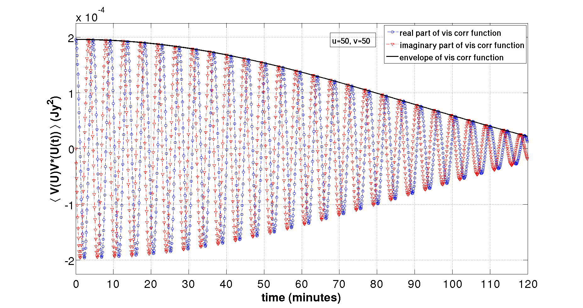
Figure 1: Visibility Correlation function as a function of time for zenith drift from equator (latitude=0). Blue and red curves correspond to the real and imaginary part of the visibility correlation function respectively. Black curve denotes the envelope of the Visibility correlation function. In the figure (and all the subsequent figures that display the visibility correlation) the visibility correlation corresponds to the HI signal from EoR computed using the power spectrum of Beardsley et al. 2013 (Figure 4 of their paper), [1]. The central frequency is assumed to be $\nu=129$ MHz.

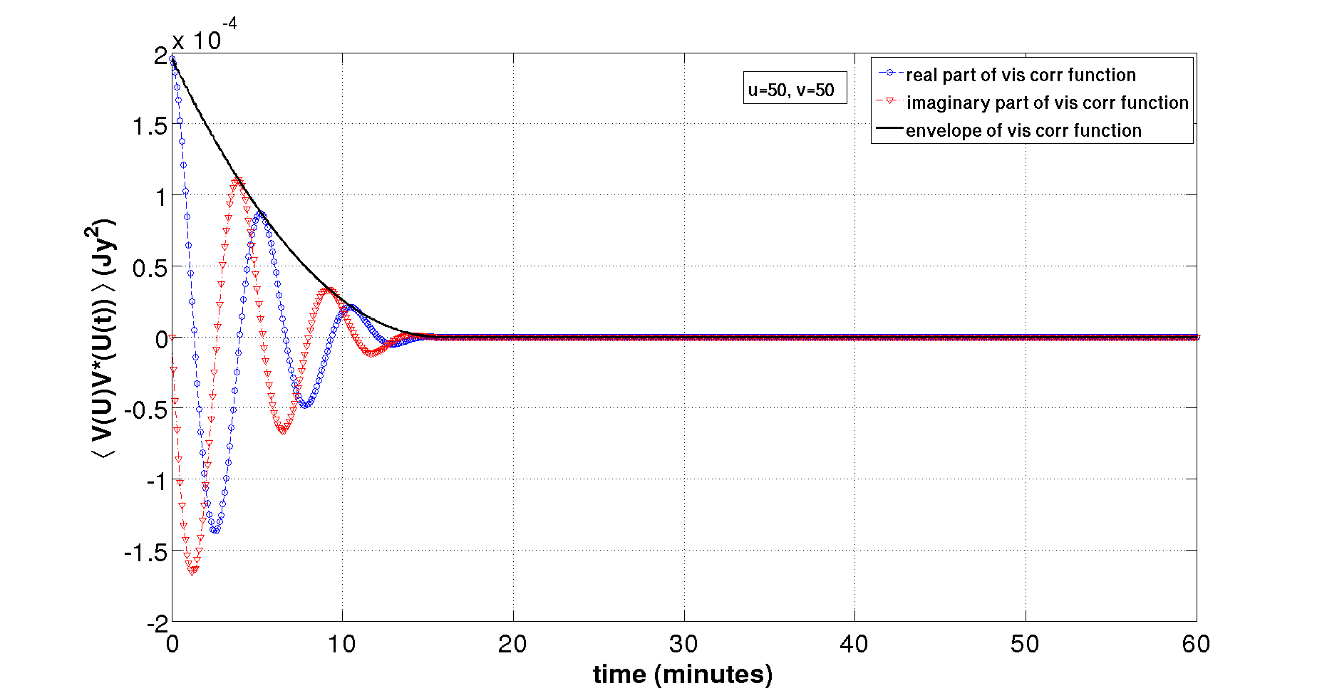
Figure 2: Visibility Correlation function as a function of time for zenith drift from a location with latitude ±$30^{\circ}$

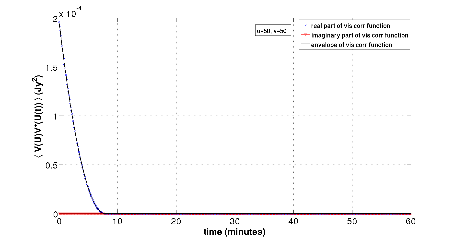
Figure 3: Visibility Correlation function as a function of time for zenith drift from the pole (latitude=±$90^{\circ}$)

It is clear that at the equator the visibilities measured by the same pair of antennas are correlated for the longest period of time. With increasing latitude of the observer the correlation time scale decreases and it is minimum for an observer at the pole (latitude 90 degree). During a drift scan, the baselines and primary beam remains fixed and the sources move in and out of the primary beam. As we show in Appendix A, the motion of sources during a scan is a combination of translation and rotation depending on the observer location and the field being observed. At the equator, the drift corresponds to pure translation along east-west axis. From any other location there also exists a rotational component in the zenith drift. The decorrelation time scale is shorter when the rotational component is present. This behaviour can be understood from Eq. (LABEL:viscorrfin1). Unless $\phi=0$, a baseline $u$ gets contribution from from not just $k_{\perp 1}$ but also $k_{\perp 2}$, the mode perpendicular to $u$ in the tracking case. A similar inference holds for $v$. This results in decorrelation time scale much shorter than the transit time of the primary beam: $\Delta h\simeq 1/(\sin(\phi)U\theta_{0})$, $\theta_{0}$ is the approximate angular extent of the primary beam. For pure translation, the decorrelation time scale depends only on the transit time of the primary beam.

Of the three fiducial cases we have studied (Figure 1–3), Figure 2 is directly relevant for the location of MWA. It is worthwhile to ask whether we could exploit the long time correlation of the equatorial scan using MWA by scanning an equatorial region. In Appendix A, we show that if the phase center is shifted to the equatorial position (along the local meridian) then with respect to the new phase center the drift is pure translation and the decorrelation due to the rotation can be avoided for this phase center. For a detailed discussion see the Appendix A and Figures (13, 14).

For an observatory at latitude $\phi$ the visibility correlation function with respect to the new phase center can be written as (Eq. (LABEL:vvlmn_prime)):

$$\langle V_{\nu}({\bf U})V^{*}_{\nu^{\prime}}({\bf U},t)\rangle = \bar{I_{\nu}}^{2}\int\frac{d^{3}k}{(2\pi)^{3}}P_{HI}(k)e^{ik_{\parallel}\Delta r_{\nu}}\exp\left(-ir_{\nu^{\prime}}k_{\perp 1}\cos(\theta+\phi)dH\right)$$

$$\>a\left[\left(u-\frac{r_{\nu}k_{\perp 1}}{2\pi}\right),\left(v-\frac{r_{\nu}k_{\perp 2}}{2\pi}\right)\right]$$

$$\>a\left[\left(u-\frac{r_{\nu}}{2\pi}(k_{\perp 1}+k_{\perp 2}\sin(\theta+\phi)dH)\right)\right.,$$

$$\>\left.\left(v-\frac{r_{\nu}}{2\pi}(k_{\perp 2}-k_{\perp 1}\sin(\theta+\phi)dH)\right)\right]$$

Here $\theta$ is the angular distance of the new phase center from zenith for an observatory at latitude $\phi$. To shift the phase center to the equator the rotation angle is $\theta=-\phi$. For this phase center, the time dependence of the visibility correlation follows the behaviour seen in Figure 1 or formally Eq. (LABEL:vvlmn) with $\phi=0$ yields the same result as Eq. (LABEL:vvlmn_prime) with $\phi=-\theta$. In other words, the two cases—an observatory located at the equator performing a zenith drift scan and an observatory located at some other latitude scanning a region at the equator–are equivalent.

In Figure 5, the time evolution of the visibility correlation function is shown for four different baselines for the equatorial scan.

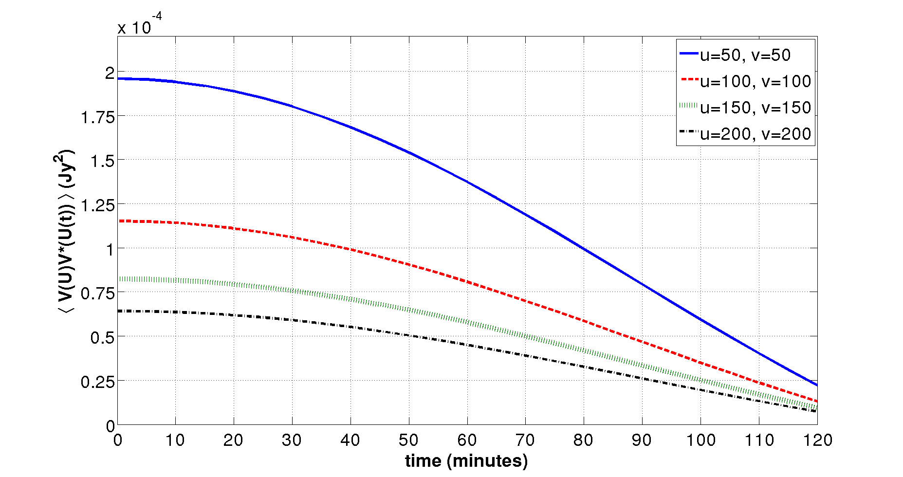
Figure 4: Envelope of Visibility Correlation function as a function of time in drift scan mode for four different baselines. The phase center is at zenith for an observer at the equator.

For observing frequency $\nu=129$ MHz and $\nu^{\prime}=\nu$ the visibility correlation is $\simeq 10^{-4}$Jy² for baselines $|{\bf U}|\leq 200$. The signal strength decreases with increasing baseline length. Figure 5 also shows that the decorrelation time scale depends only the size of the primary beam for an equatorial scan.

3.1 Correcting for Rotation

In figures (2) and (3) one sees that the rotation of sources in the sky plane during the drift scan reduces the time scale of decorrelation of visibility correlation function for a given baseline.

In a drift scan, the phase center remains fixed and therefore there is no change in the values of {u,v,w}. In other words, the set of baselines during the scan remains the same.

In the foregoing (Eq. (LABEL:viscorrfin1) and the discussion following it) we have shown that the visibilities become uncorrelated when ${\bf U}-{\bf U^{\prime}}\gtrsim 0.5$ for the MWA primary beam. In the drift scan case, this condition holds if both the visibilities are obtained at the same time. However, Eq. (LABEL:viscorrfin1) can be used to show that this conclusion doesn’t hold for visibilities computed at different times. In particular, we show that $V({\bf U},t)$ and $V({\bf U^{\prime}},t^{\prime})$ can become correlated for ${\bf U}\neq{\bf U^{\prime}}$ and $t\neq t^{\prime}$, if the two baselines are related by a special relation. We derive this relation and illustrate this re-correlation with an example.

Two baselines ${\bf U}=(u,v)$ and ${\bf U^{\prime}}=(u^{\prime},v^{\prime})$ can be related as:

$$u^{\prime}=u+av+\varepsilon$$

$$v^{\prime}=v-au+\varepsilon$$

Here a and $\epsilon$ correspond to rotation and translation respectively. These parameters can be solved to give:

$$a=\frac{\Delta u-\Delta v}{u+v}$$

$$\varepsilon=\frac{u\Delta u+v\Delta v}{u+v}$$

Here ${\bf\Delta U}={\bf U}-{\bf U^{\prime}}$.

It can be shown that for two baselines with $\varepsilon\geq 0.5$ the signal gets uncorrelated and cannot be re-correlated at any other time. This also means that two baselines with different lengths $(u^{2}+v^{2})^{1/2}$ remain uncorrelated during the drift scan. However, many baselines in an experiment such as MWA have nearly the same lengths and are related to each other by a near pure rotation denoted by the parameter $a$. We can show that such baselines correlate with each other during the drift scan if $a=\sin(\phi)dH$. In other words, if a visibility is measured at a time $t=0$ for a baseline ${\bf U}$, then this measurement will correlate with another measurement for a baseline ${\bf U^{\prime}}$ at a time corresponding to $dH$ if the two baselines are related by a near pure rotation with the corresponding rotation parameter $a=\sin(\phi)dH$. We note that this correlation can occur just once during a long scan and the time scale over which the baselines remain correlated corresponds to the decorrelation time for a given $|{\bf U}|$.

We illustrate this re-correlation for a baseline ${\bf U}=(35,10)$. The other baseline ${\bf U^{\prime}}=(34.8,10.7)$ corresponds to parameters $a=-0.02$, $\varepsilon=0$. The visibility correlation function is shown as a function of time in Figure 5.

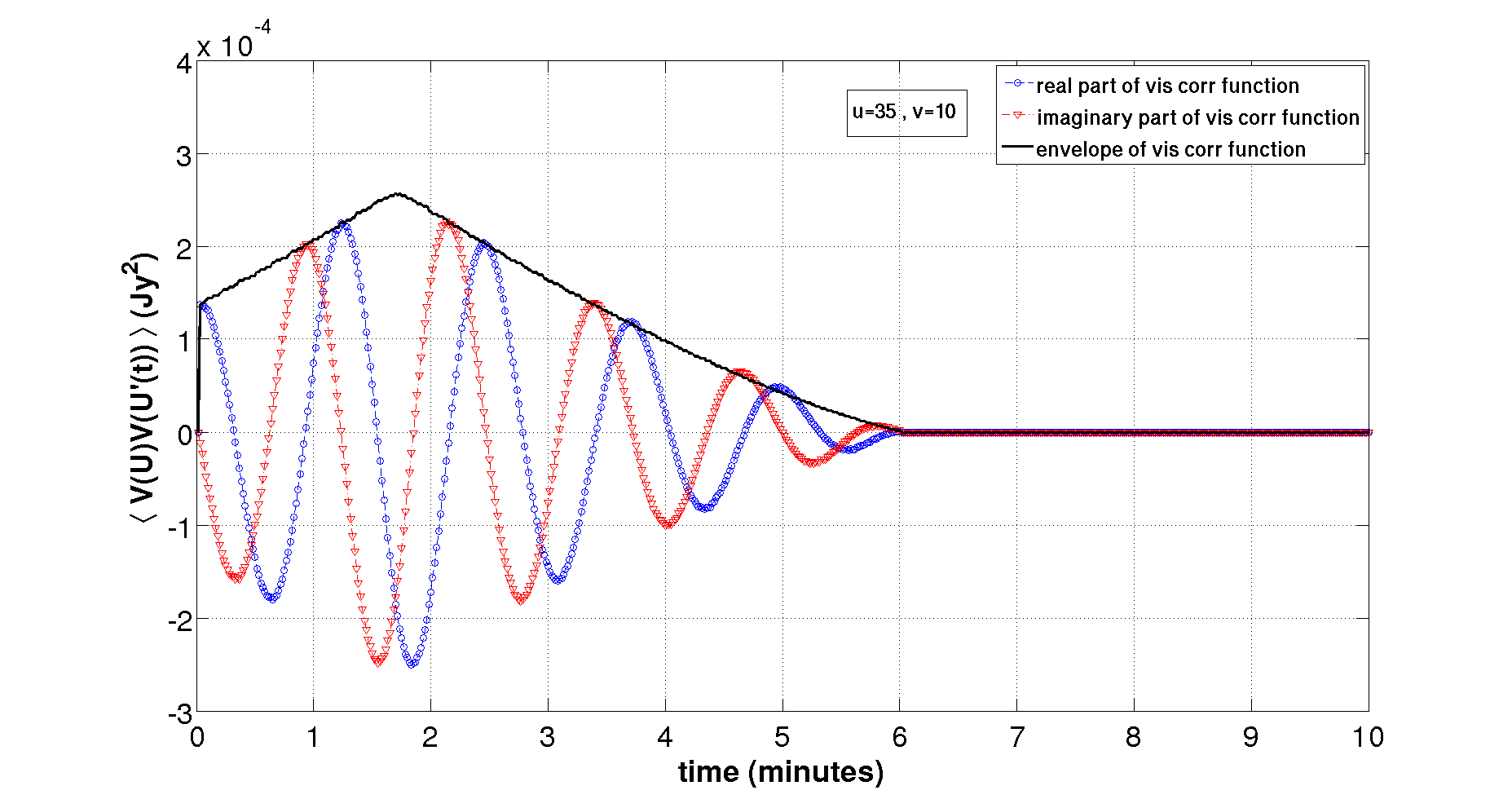
Figure 5: Visibility correlation function as a function of time for visibilities with different baselines. The drift scan correspond to a zenith scan for a latitude of $30^{\circ}$

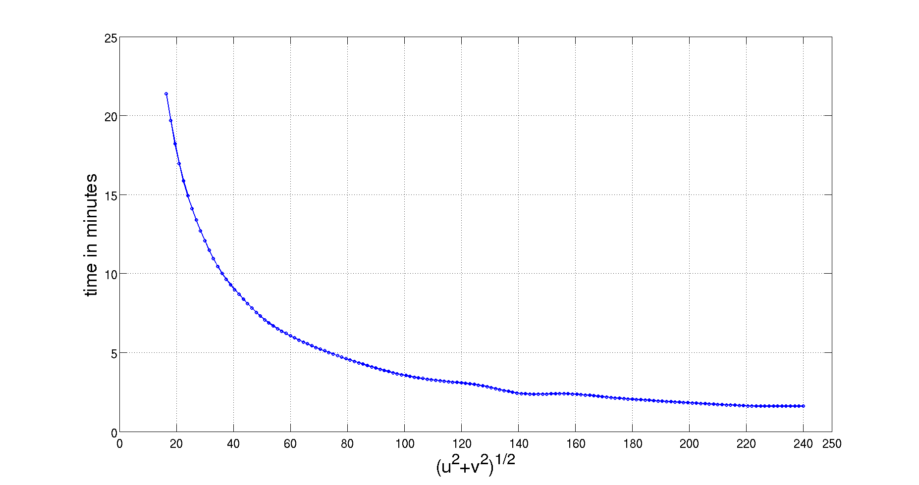
Figure 6: The Figure displays the time difference $\Delta$t at which the visibility correlation falls to half its value, as a function of baseline, for an overhead scan at the location of MWA ($\phi=-26.7$).

In Figure 6 we show the time scale over which the visibility correlation falls to half its value for $\Delta t=0$ (e.g. Figure 2); this time scale is seen to fall as roughly the inverse of the baseline length, in agreement with the discussion in the previous sub-section.

The re-correlation of baselines allows us to partially recover the loss of signal due to decorrelation. However, the set of baselines is fixed for a drift scan strategy and therefore the range of baselines that correlate at different times must be present in the initial set. For the MWA, we estimate that for a zenith scan at the latitude of the telescope there are nearly 120 such pairs which satisfy $\varepsilon\leq 0.5$ and $a\leq 0.3$ for $|{\bf U}|\simeq 20\hbox{--}70$. (as noted below, the total number of baselines in a zenith snapshot observation for MWA is 2735 in the range $|{\bf U}|\simeq 20\hbox{--}230$.) These baselines will retain at least half the signal and would correlate within a correlation time scale of less than two hours.

4 Error on visibility correlation

The error on visibility correlation is:

$$\sigma^{2}(U)=\langle V_{\nu}({\bf U})V_{\nu}({\bf U})V_{\nu^{\prime}}({\bf U^{\prime}},t)V_{\nu^{\prime}}({\bf U^{\prime}},t)\rangle-\langle V_{\nu}({\bf U})V_{\nu^{\prime}}({\bf U^{\prime}},t)\rangle^{2}$$ (17)

Here $U\equiv|{\bf U}|$ and the averages are taken over many different variables: the noise is uncorrelated for different frequencies, baselines, and times. However, the signal could be correlated in all the three domains. We average over all the pairs in the three domains and finally over all the pairs for baselines in the range $U$ and $U+{\Delta}U$ to compute an estimate for a wider bin $\Delta U$. The measured visibilities and their correlations receive contributions from detector noise, the HI signal, and the foregrounds. When only visibilities at two times (or frequencies/baselines) are correlated, as we assume here, the $\langle VV\rangle$ doesn’t receive any contribution from detector noise and therefore constitutes an unbiased estimator of the signal. In this case, only the first term in the equation above contributes to the error estimate; denoting the sky noise as $N_{\nu}$, we get:

$$\sigma^{2}(U)={1\over N_{\rm tot}}\langle N_{\nu}({\bf U})N^{*}_{\nu}({\bf U})\rangle^{2}$$ (18)

Here $N_{\rm tot}$ are all the baseline pairs in the range $U$ and $U+{\Delta}U$ in the three-dimensional cube and the time domain.

The average noise autocorrelation for each independent correlation of visibilities is:

$$\langle N_{\nu}({\bf U})N^{*}_{\nu}({\bf U})\rangle=\left[\frac{T_{\rm sys}}{K\sqrt{\Delta\nu\Delta t}}\right]^{2}$$ (19)

where $T_{\rm sys}$ is the system temperature, $\Delta\nu$ is the channel width, K is the antenna gain and $\Delta t$ is the integration time. Here $\Delta t$ and $\Delta\nu$ could be arbitrarily small; in particular we require the bandwidth and integration time to be much smaller than the frequency and time coherence of the signal (Figure 1–3 and 6). $N_{\rm tot}$ is determined from the correlation times scale in time and frequency domains and its computation is discussed below. We cross-correlate all visibility pairs for a given time difference and frequency difference for the equatorial scan case where we assume ${\bf U}={\bf U^{\prime}}$; we also include the impact of re-correlating baselines (section 3.1) in the overhead scan case (Figure 2).

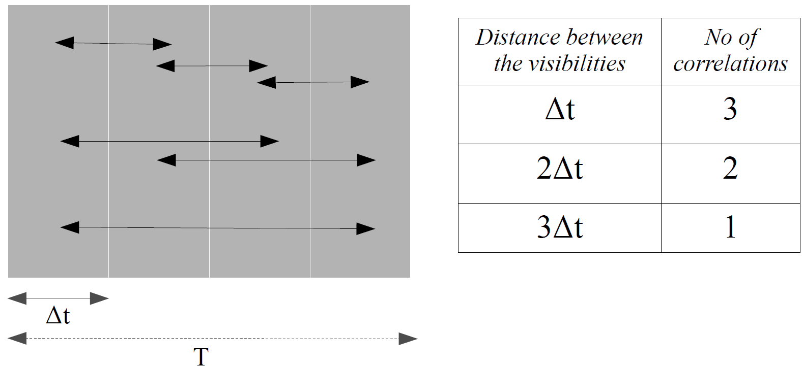
Figure 7: Illustration showing the number of possible correlations for total observing time T and integration time $\Delta t$ with $T/\Delta t=4$, or four visibility measurements. The number of correlations between visibilities with time difference $\Delta t$ is four, for time difference $2\Delta t$ the number is three and so on.

For a given total observing time T and integration time $\Delta t$, there exists $n=T/\Delta t$ visibility measurements. Among these, the number of possible independent correlations between visibilities $i\Delta t$ time apart (where i=1,2,….,n) is $(n-i)$ as explained in figure 7. Thus, average noise correlation for a given baseline vector U with visibilities separated by times $i\Delta t$ is:

$$\sigma_{i}({\bf U})=\langle N_{\nu}({\bf U})N^{*}_{\nu}({\bf U}(i\Delta t))\rangle=\frac{1}{(n-i)}\left[\frac{T_{sys}}{K\sqrt{\Delta\nu\Delta t}}\right]^{2},$$ (20)

for any frequency channel.

Figure 4 shows that the signal $\sqrt{\langle V_{\nu}({\bf U})V^{*}_{\nu^{\prime}}({\bf U^{\prime}},t)\rangle}$ decorrelates with increasing time difference between the visibilities. This means that not all pairs contribute equally to the signal-to-noise of the measurement. To obtain an estimator that gives suitable weight to all the pairs we define:

$$w_{i}({\bf U})=\frac{\langle V_{\nu}({\bf U})V^{*}_{\nu}({\bf U}(t=0))\rangle}{\langle V_{\nu}({\bf U})V^{*}_{\nu}({\bf U}(t=i\Delta t))\rangle}$$ (21)

This allows us to write the following optimal estimator for computing the noise on the visibility measurement:

$$\frac{1}{(\sigma_{U}^{2})^{2}}=\displaystyle\sum_{i=1}^{n}\frac{1}{(\sigma_{i}^{2}w_{i})^{2}}$$ (22)

We neglect the effect of partial coherence of baselines at the initial time; this assumption slightly underestimates the sensitivity and is further discussed in the next subsection. We do not include sampling variance in our error estimates.

The foregoing discussion is valid for visibility measurements for a given frequency. The HI signal is correlated across frequency space (Figure 8). The figure shows the behaviour of the HI signal as a function of $|\nu^{\prime}-\nu|$ for different baselines. The right panel of the figure displays the frequency difference at which the signal falls to half of the of the maximum ($|\nu^{\prime}-\nu|=0$) for different times. We treat the correlation across the frequency space using the same method described above for the time correlation.

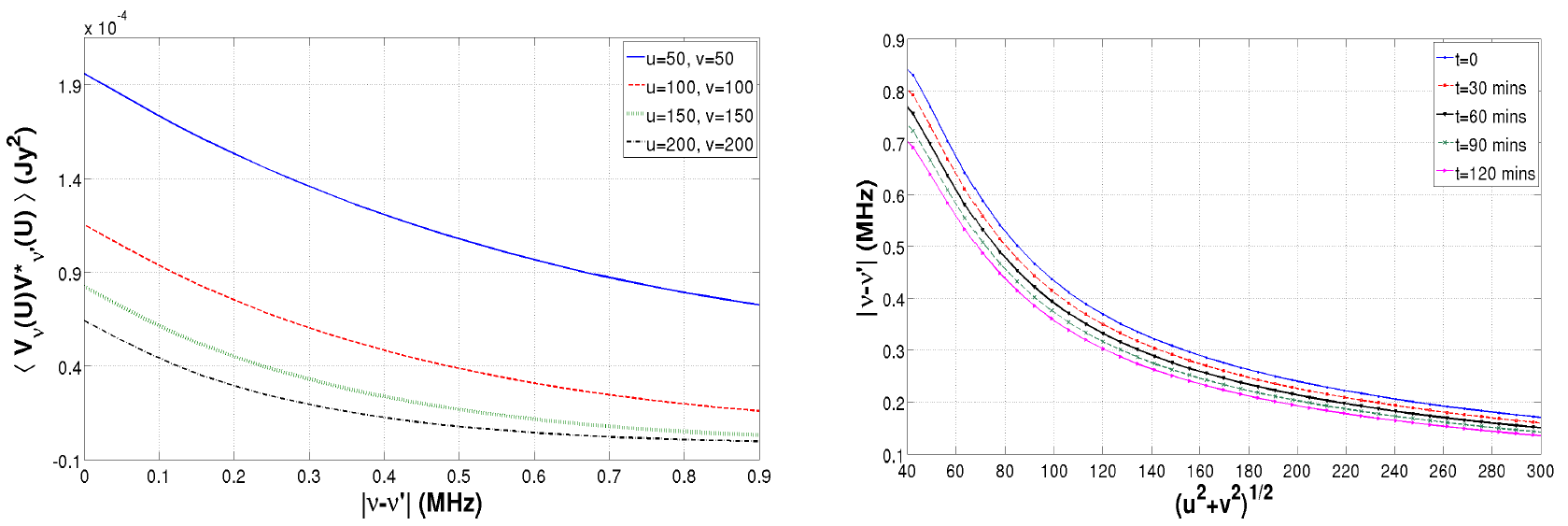
Figure 8: The left figure shows the decorrelation of visibility correlation of the HI signal as a function of frequency separation (see the caption of Figure 1 and the discussion in section 3 for details). The right panel denotes the bandwidth for a given U at which the signal drops to half of its maximum at different times

In Figure 9, we show the expected noise on the visibility correlation for many different cases. For all the cases, we assume the following parameters for the MWA: observing frequency $\nu=129$ MHz, system temperature $T_{\rm sys}=440$ K, and the effective area of each tile $A_{\rm eff}=16m^{2}$.

Case-I: We consider a continuous equatorial drift scan of a duration of 2 and 4 hours. One way to repeat the scan for the same phase center is to shift the phase center to the same position after the end of the scan; this results in the change of UV coverage. We consider the simpler case when the UV coverage and the phase center remain the same for subsequent scans. This corresponds to the same region of sky being observed on different days. In Figure 9 we show the results for 900 hours of integration in this mode.

As the signal strength is greater for shorter baselines (figure 4), we consider only baselines in the range ${\bf U}=20\hbox{--}230$. We take bins of size ${\bf U}\simeq 10$ and show the noise correlation for this range of baselines in Figure 9. MWA has 2735 baselines in this range for a snap-shot observation. Using the information, the RMS noise for this mode is $\sigma\simeq 16$ (mJy)² and $\sigma\simeq 21$ (mJy)² for 2 and 4 hours scan, respectively. We note that since the visibility correlation function drops significantly after roughly 1 hour (Figure 1), the noise is expected to increase for longer drift scans.

Case-II: Here we consider an overhead drift scan at the location of MWA. The correlation time scale is shorter for such scans as compared to the equatorial scan (Figure 2). In Figure 6 we show the time scale over which the correlation falls by half as a function of the baseline length.

As noted above many baselines get re-correlated as the time progresses (Figure 5). Over 5–10% of all the baselines in the range $|{\bf U}|=20\hbox{--}100$ get re-correlated with $\epsilon\leq 0.5$ in less than two hours. We include these baselines in the noise computation. As compared to Case I, the noise is higher in this case as the correlation time is shorter.

Case-III: For comparison with the drift scan cases, we also compute the error in the visibility correlation for the tracking case. We consider two cases: 2 and 6 hours continuous tracking of a region across the zenith ($\pm 1$h and $\pm 3$h) at the location of MWA ($\phi=-26.7$). The results are shown Figure 9. We discuss the results in detail in the next subsection.

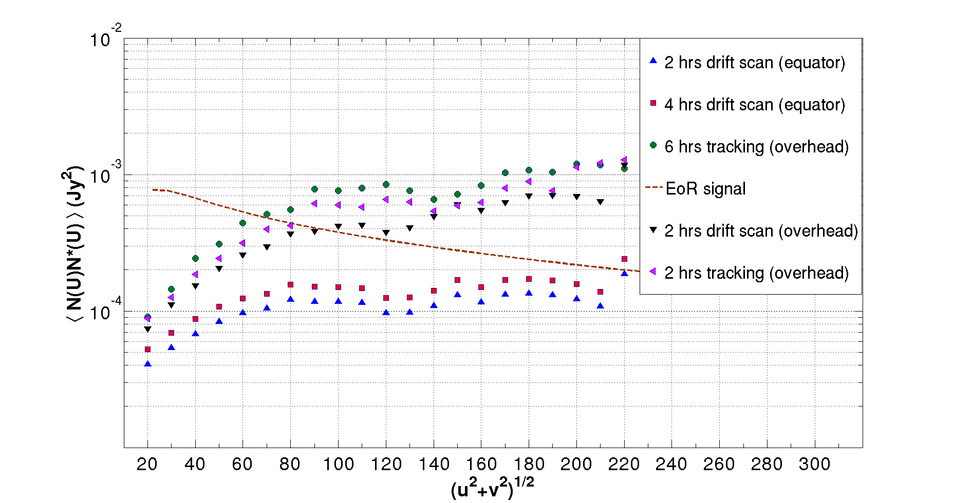
Figure 9: Error on visibility correlation as a function of baseline length: blue (triangle) and red (square) points refer to 2 and 4 hours equatorial drift scans, respectively. Black (inverted triangle) points refer to 2 hours zenith drift scan at the location of MWA. The green (circle) and pink (rotated triangle) points show the expected error for 2 and 6 hour tracking runs (for $\pm 3$ and $\pm 1$ hour continuous overhead tracking at MWA location). In all the cases the total integration is 900 hours. The EoR signal is designated by the dashed brown line.

4.1 Drift vs tracking mode

In any interferometric experiment to determine the EoR signal, the RMS noise on the visibility correlation is bounded by:

$$\sigma_{\rm min} = \left({1\over N_{b}}\right)^{1/2}\left({T_{\rm sys}K\over\sqrt{\Delta\nu T}}\right)^{2}$$ (23)

$$\sigma_{\rm max} = \left({\Delta t\over N_{b}T}\right)^{1/2}\left({T_{\rm sys}K\over\sqrt{\Delta\nu\Delta t}}\right)^{2}.$$ (24)

Here $T$ is the total time of integration and $\Delta t$ is the integration time for a single visibility measurement. For the sake of the discussion, $\Delta\nu$, the channel width is assumed to be fixed. $N_{b}=n(n-1)/2$ is the total number of baselines for any measurement with n antenna elements. $\sigma_{\rm min}$ gives the RMS noise if all the visibilities are coherently added and $\sigma_{\rm max}$ corresponds to the case when the visibility correlations are incoherently added. For the 128-tile MWA, the RMS lies between these two extremes for both the tracking mode and drift scans. As noted above, we neglect partially coherent baselines for computing the sensitivity for drift scans; this assumption is consistent with Eq (23).

The process of decoherence occurs differently for the tracking and the drift scan mode. For drift scans, it is decorrelation of the EoR signal at different times, as described in detail in the previous sections. In the tracking case, the process of tracking a given region rotates the visibility vector ${\bf U}$; the correlation between visibility measurements at different values of ${\bf U}$ decreases; from Eq. (LABEL:crosscor), we can show that the decorrelation scale $\Delta{\bf U}\simeq\theta_{0}^{-1}\simeq 0.5$ has very weak dependence on the value of ${\bf U}$. For our computation we take the pixel size: $\{\Delta U,\Delta V\}=\{0.5,0.5\}$. The frequency decorrelation for the tracking case is taken from figure 8.

The results for two and six hour tracking runs (zenith at the location of MWA) are shown for 900 hours of integration in figure 9. We note here that we do not present the results for equatorial tracking run, as the sensitivity in this case shows only a marginal improvement over the zenith tracking runs shown in Figure 9. As the figure shows, the drift scan generally gives lower noise on the visibility correlation for up to 4 hours of drift scans.

This result can be understood as follows. As an extreme case, one could drift for a very short duration each day, such that there is no decorrelation and continue similar observations on the same field such that all the visibility measurements are coherently added. In this case, the RMS for the drift case would approach $\sigma_{\rm min}$ which is not possible to achieve in the tracking case because the process of tracking would always decorrelate the signal. The relevant question is: what is the time scale for drift scans such that this advantage of lower noise is not lost. We show that even for four-hour drift scans this advantage holds. In the drift scan case, the decorrelation time scale is $\simeq 1$hour. In the tracking cases, different baseline decorrelate in the process of tracking a region of the sky but some baselines revisit the same pixel in this process. For instance, for a six hour tracking run shown in Figure 9, the average integration time of a pixel in the range: $|{\bf U}|=20\hbox{--}30$ is roughly 15 minutes with the total number of uncorrelated pixels $\simeq 4700$.

It should be underlined that, apart from other assumptions delineated in the previous sub-section, the lower noise in the drift scan is also based on the assumption that the system temperature doesn’t change over the scan. Also an additional disadvantage in the drift scan case is that there are smaller number of visibility measurements available at any given time for imaging as compared to the tracking case where the UV coverage is better.

5 Statistical homogeneity of EoR signal and foreground extraction

Unlike the tracking case, the drift scans explicitly exploit the statistical homogeneity of the EoR signal: cross correlation of the signal at different times only depends on the time difference. More precisely, the power spectrum of the EoR signal for any phase center is drawn from a random density field with the same average power spectrum. This assumption may or may not hold for foregrounds. For instance, if faint point sources are distributed homogeneously across the sky with the same flux distribution, they will also closely correspond to a statistically homogeneous field in two dimensions. However, most other foregrounds, e.g. bright point sources or galactic foregrounds, will explicitly break the statistical homogeneity of the sky and therefore would be potentially distinguishable from the EoR signal.

We illustrate this concept with point source distribution on the sky. For a point source distribution with fluxes $\{F_{i}\}$, the visibility can be written as:

$$V({\bf U})=\sum_{j}\exp(2\pi i{\bf U}.{\bf\theta_{j}}(t))F_{j}A({\bf\theta_{j}}(t))$$ (25)

Here ${\bf\theta_{i}}(t)$ correspond to the time varying position of point sources on the sky with respect to the fixed phase center. $A({\bf\theta_{i}}(t))$ gives the primary beam in the same coordinate system. The visibility correlation separated by time $\Delta t$ is:

$$\langle V({\bf U},t)V^{*}({\bf U},t+\Delta t)\rangle=\langle\sum_{k}\sum_{j}\exp(2\pi i{\bf U}.({\bf\theta_{j}}-{\bf\theta_{k}}))F_{j}F_{k}A({\bf\theta_{j}}(t))A({\bf\theta_{k}}(t+\Delta t))\rangle$$ (26)

Here the averaging process $\langle\cdots\rangle$ is over all the pairs for a given $\Delta t$ during the drift scan. This averaging procedure leads to substantially different results for the EoR signal and the foregrounds: the EoR signal is statistically homogeneous and therefore any cross-correlation depends only on $\Delta t$. For each $\Delta t$ the EoR signal gives a realization of the density field with a given fixed power spectrum (Eq. (LABEL:crosscor)). However, the foregrounds might not share this property and might show explicit dependence not just the time difference but the time period of the scan. This gives at least two different methods of extracting foregrounds: (a) correlation pairs of a given $\Delta t$ can be used to fit the time variation expected of foregrounds. While the EoR signal will show fluctuations about a given mean, the foregrounds will show more secular time variation which can potentially be subtracted, (b) direct comparison of the averaged correlation function should also reveal the difference between the two cases. We demonstrate the procedure with method (b) here.

For MWA primary beam, we consider three different source counts: 10, 30 and 50 sources. At the beginning of the drift scan the sources are randomly distributed within ±$15^{\circ}$ from the center of the primary beam with hour angle between -3 to +3 hours. The fluxes are drawn from uniform distribution with values between 0 and 1 Jy. The visibility correlation function for all these cases for U=(50,50) are shown in figure 10.

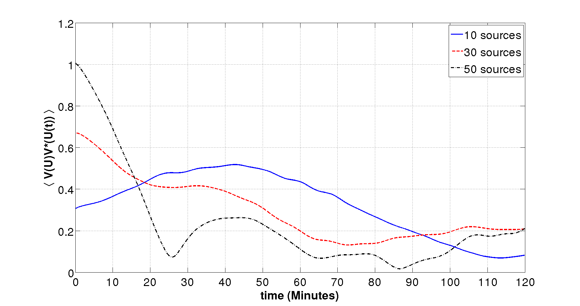
Figure 10: Envelope of the Visibility correlation function (normalized arbitrarily) as a function of time difference for three different cases described in the text.

As predicted in the foregoing, figure 10 shows that the visibility correlation function for point sources is substantially different as compared to the HI signal owing to statistical inhomogeneity of the point source distribution. This can be used to subtract the contribution of bright point sources from the measured visibility itself.

6 Conclusions

The main goal of this paper is to investigate the potential of the drift scan technique in estimating the EoR signal. Drift scans introduce a new dimension to the issue: the correlation between visibilities in time domain. Here we present a formalism which uses this correlation to determine the EoR signal.

The important results are as follows:

• The visibilities measured at different times by the same pair of antennas in a drift scan are correlated for up to 1 hour for equatorial scans (Figure 1). The decorrelation time scale depends on the choice of phase center. It is maximum for an equatorial zenith drift or for equatorial phase center. For such scans, the decorrelation time scale is independent of the baseline length. For other scans the decorrelation times scale is shorter and depends on the baseline vector (Figure 2–3). However, a fraction of these baselines correlate with other baselines at a different time (Figure 5).

• We compute the expected error on the visibility correlation for drift scans and compare with the expected noise in the tracking case (Figure 9). Our results show that the noise is comparable in the two cases and the drift scan might lead to a superior signal-to-noise for equatorial scans.

• The drift scan technique also opens another avenue for the extraction and subtraction of foregrounds: the EoR signal is statistically homogeneous while the foregrounds might not share this property. We investigate the potential of this possibility using a set of bright point sources (figure 10).

Our results suggest that drift scans might provide a viable, and potentially superior, method for extracting the EoR signal. In this paper, we present mainly analytic results to make our case. In the future, we hope to return to this issue with numerical simulations and direct application of our method to the MWA data.

Acknowledgments: We thank Rajaram Nityananda, Ron Ekers, Sanjay Bhatnagar, Urvashi Rau, Nithyanandan Thyagarajan, Subhash Karbelkar for the useful comments and discussions. We thank the referee for penetrating comments which helped us to improve the paper.

This scientific work makes use of the Murchison Radio-astronomy Observatory, operated by CSIRO. We acknowledge the Wajarri Yamatji people as the traditional owners of the Observatory site. Support for the MWA comes from the U.S. National Science Foundation (grants AST-0457585, PHY-0835713, CAREER-0847753, and AST-0908884), the Australian Research Council (LIEF grants LE0775621 and LE0882938), the U.S. Air Force Office of Scientic Research (grant FA9550-0510247), and the Centre for All-sky Astrophysics (an Australian Research Council Centre of Excellence funded by grant CE110001020). Support is also provided by the Smithsonian Astrophysical Observatory, the MIT School of Science, the Raman Research Institute, the Australian National University, and the Victoria University of Wellington (via grant MED-E1799 from the New Zealand Ministry of Economic Development and an IBM Shared University Research Grant). The Australian Federal government provides additional support via the Commonwealth Scientific and Industrial Research Organisation (CSIRO), National Collaborative Research Infrastructure Strategy, Education Investment Fund, and the Australia India Strategic Research Fund, and Astronomy Australia Limited, under contract to Curtin University. We acknowledge the iVEC Petabyte Data Store, the Initiative in Innovative Computing and the CUDA Center for Excellence sponsored by NVIDIA at Harvard University, and the International Centre for Radio Astronomy Research (ICRAR), a Joint Venture of Curtin University and The University of Western Australia, funded by the Western Australian State government.

7 Appendix

Appendix A Coordinate system for drift scans

The position vector in the sky $\vec{\theta}$ can be expressed in terms of two direction cosines l and m. These direction cosines are defined with respect to a local coordinate system when phase center is at zenith as explained in figure 11 (e.g. [5]):

$$l = \cos\delta\sin H$$

$$m = \cos\delta\cos H\sin\phi-\sin\delta\cos\phi$$

$$n = \cos\delta\cos H\cos\phi+\sin\delta\sin\phi$$ (27)

Here $\delta$ and H are the declination and hour angle of any source; and $\phi$ is the latitude of the place of observation.

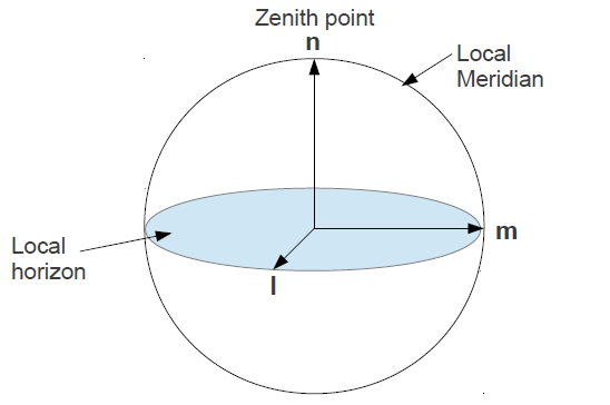
Figure 11: l,m,n coordinates defined for a phase center at zenith

Using this coordinate system the second integral in visibility expression Eq. (LABEL:viscorrt) takes the form:

$$\int dldmA(l,m)\exp\left[-2\pi i\left\{\left(u-\frac{k_{\perp 1}r_{\nu}}{2\pi}\right)l+\left(v-\frac{k_{\perp 2}r_{\nu}}{2\pi}\right)m\right\}\right]\exp\left[-ir_{\nu}\left(k_{\perp 1}\Delta l+k_{\perp 2}\Delta m\right)\right]$$ (28)

Here $\Delta l$ and $\Delta m$ are the change in $l$ and $m$ with time or hour angle as in sky drift only hour angle changes with time for a fixed declination. $k_{\perp 1}$ and $k_{\perp 2}$ are the two components of ${\bf k}_{\perp}$ along $l$ and $m$ on the sky plane. Using Eq. (27) and the condition $l^{2}+m^{2}+n^{2}=1$ we can expand in the first order to compute the changes in relevant quantities:

$$\Delta l=(m\sin\phi+n\cos\phi)dH;\hskip 15.0pt\Delta m=-(l\sin\phi)dH.$$ (29)

Here dH is the change in hour angle in time interval $t$. We can further simplify the expression by using $n\simeq 1$. The two approximation used above are: $1/2(l^{2}+m^{2})\ll 1$ and $dh\ll 1$. Both these approximations are valid for the MWA primary beam (Eq. (14)) and for a few hours of correlation time. Thus the second integral (Eq. 27) becomes:

$$\exp\left(-ir_{\nu}k_{\perp 1}\cos\phi dH\right)\int dldmA(l,m)\exp\left[-2\pi i\left\{\left(u-\frac{r_{\nu}}{2\pi}(k_{\perp 1}+k_{\perp 2}\sin\phi dH)\right)l\right.\right.$$

$$\left.\left.+\left(v-\frac{r_{\nu}}{2\pi}(k_{\perp 2}-k_{\perp 1}\sin\phi dH)\right)m\right\}\right]$$

It can be expressed in terms of the Fourier transform of the primary beam:

$$\exp\left(-ir_{\nu}k_{\perp 1}\cos\phi dH\right)a\left[\left(u-\frac{r_{\nu}}{2\pi}(k_{\perp 1}+k_{\perp 2}\sin\phi dH)\right),\left(v-\frac{r_{\nu}}{2\pi}(k_{\perp 2}-k_{\perp 1}\sin\phi dH)\right)\right]$$ (30)

With this the visibility measured at a later time $t$ becomes:

$$V_{\nu}({\bf U},t) = \bar{I}_{\nu}\int\frac{d^{3}k}{(2\pi)^{3}}\Delta_{HI}({\bf k})e^{ir_{\nu}k_{\parallel}}\exp\left(-ir_{\nu}k_{\perp 1}\cos\phi dH\right)$$ (31)

$$\>a\left[\left(u-\frac{r_{\nu}}{2\pi}(k_{\perp 1}+k_{\perp 2}\sin\phi dH)\right),\left(v-\frac{r_{\nu}}{2\pi}(k_{\perp 2}-k_{\perp 1}\sin\phi dH)\right)\right]$$

Correlating this with the visibility measured at t=0 (equation 7) gives:

$$\langle V_{\nu}({\bf U})V^{*}_{\nu^{\prime}}({\bf U^{\prime}},t)\rangle = \bar{I_{\nu}}^{2}\int\frac{d^{3}k}{(2\pi)^{3}}P_{HI}(k)e^{ik_{\parallel}\Delta r_{\nu}}\exp\left(-ir_{\nu^{\prime}}k_{\perp 1}\cos\phi dH\right)$$

$$\>a\left[\left(u-\frac{r_{\nu}k_{\perp 1}}{2\pi}\right),\left(v-\frac{r_{\nu}k_{\perp 2}}{2\pi}\right)\right]$$

$$\>a\left[\left(u^{\prime}-\frac{r_{\nu}}{2\pi}(k_{\perp 1}+k_{\perp 2}\sin\phi dH)\right),\left(v^{\prime}-\frac{r_{\nu}}{2\pi}(k_{\perp 2}-k_{\perp 1}\sin\phi dH)\right)\right]$$

Eq. (LABEL:vvlmn) and the discussion in this section allows us to interpret Figure 1–3. If $\phi=0$, or the observatory is located at the equator, then the trajectory of sources around the phase center in a drift scan is pure translation; for any non-zero $\phi$ the motion is a combination of rotation and translation (Eq. (29). For pure translation, one obtains Figure 1, or the decorrelation time scale is determined solely by the extent of the primary beam. The decorrelation time scale is shorter for any non-zero $\phi$ (Figure 2, 3, and 6) and depends on the baseline, as already noted in section 3.

MWA is not located at the equator but we show below that, even for an observatory not located at the equator, if the phase center is shifted to an equatorial position one can remove the rotation of sources in the coordinate system constructed for the new phase center. For simplicity we construct a coordinate system around the local meridian but our conclusions remain valid for any phase center along the equator.

For a phase center that lies on the local meridian with angular separation $\theta$ from the zenith at the observatory (Figure 12), the new set of coordinate system is obtained by a single rotation $\theta$ of the m and n axes about l as shown in the figure 12.

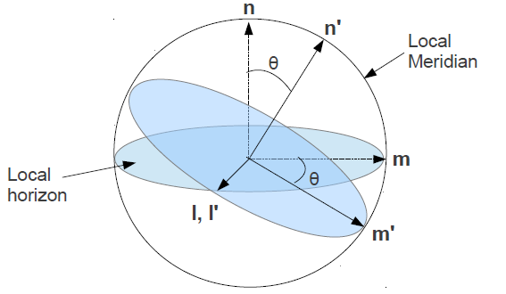
Figure 12: Illustration of new lmn coordinate system

Thus the new coordinates can be expressed as:

$$\begin{pmatrix}l^{\prime}\\ m^{\prime}\\ n^{\prime}\end{pmatrix}=\begin{pmatrix}1&0&0\\ 0&\cos\theta&\sin\theta\\ 0&-\sin\theta&\cos\theta\end{pmatrix}\begin{pmatrix}l\\ m\\ n\end{pmatrix}$$ (33)

Substituting l,m,n values from equation (27) we get:

$$l^{\prime} = \cos\delta\sin H$$

$$m^{\prime} = \cos\delta\cos H\sin(\theta+\phi)-\sin\delta\cos(\theta+\phi)$$

$$n^{\prime} = \cos\delta\cos H\cos(\theta+\phi)+\sin\delta\sin(\theta+\phi)$$ (34)

We illustrate the difference between the two coordinate systems with a set of point sources with given initial positions (hour angle and declination) and compute source trajectories in both lmn and l’m’n’ coordinates. The unprimed coordinates are for a zenith scan at the location of the observatory. The primed coordinates are for a phase center which is at equatorial position at the meridian. In this case, for on observer situated at latitude $\phi$, the angle of rotation $\theta=-\phi$. For instance for an observer at latitude $\phi=30^{\circ}$N, rotation angle is $\theta=-30^{\circ}$.

Ten sources are chosen randomly within declination ±$10^{\circ}$ of the center of the primary beam and all with initial hour angle -2h. The sources are allowed to drift past the primary beam for a total drift duration of 4 hours. The trajectories are shown figures 13 and 14. A contour plot of the primary beam is also included in each figure.

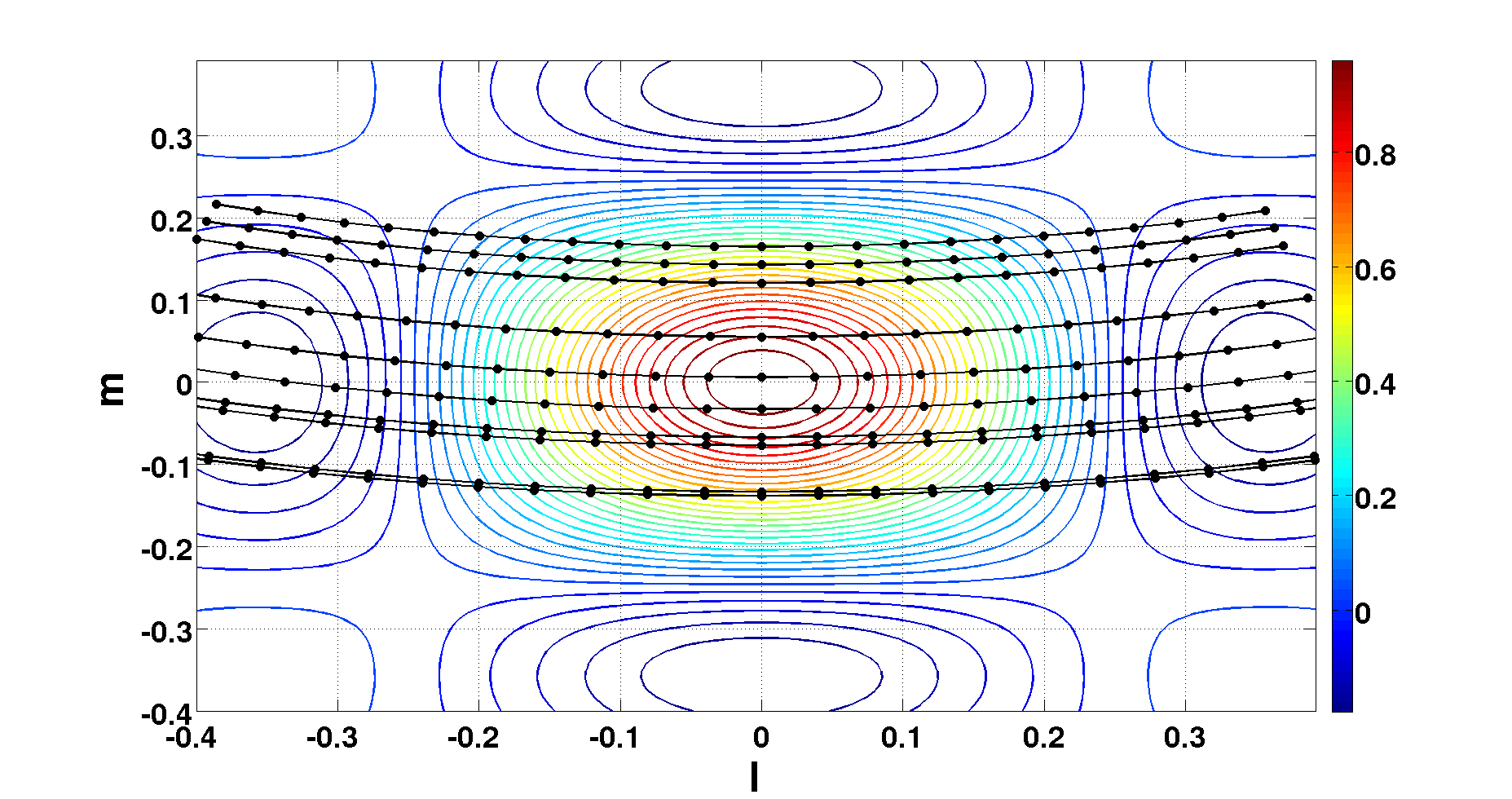
Figure 13: source trajectories in lmn coordinate system (phase center at zenith) for an observer at latitude $-30^{\circ}$

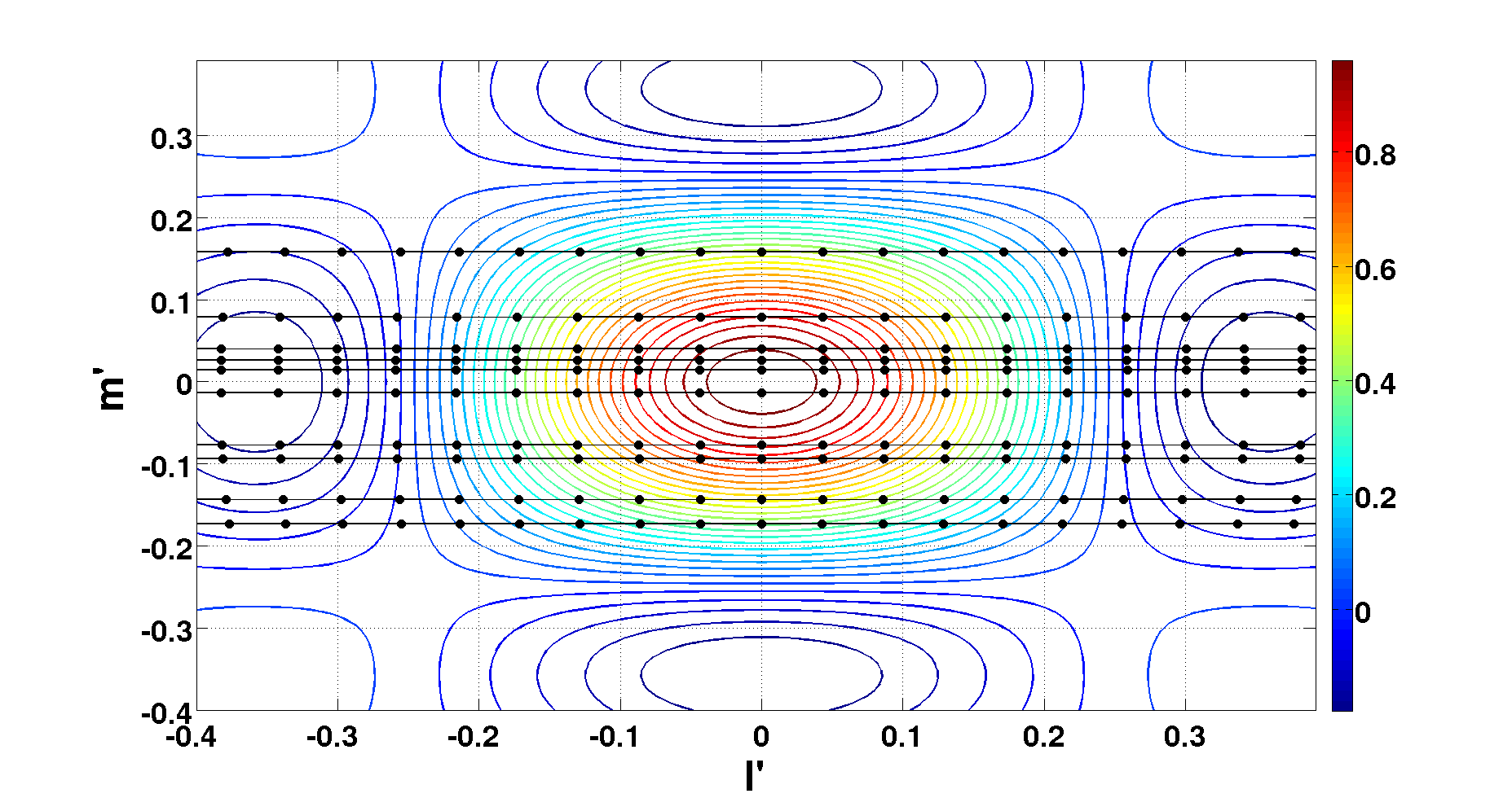
Figure 14: source trajectories in l’m’n’ coordinate system (phase center shifted to equator) for the same observer as in Figure 13

Using the new primed coordinate system instead of the previous one with phase center at zenith at the observatory, one obtains the expression for the visibility correlation function as:

$$\langle V_{\nu}({\bf U})V^{*}_{\nu^{\prime}}({\bf U^{\prime}},t)\rangle = \bar{I_{\nu}}^{2}\int\frac{d^{3}k}{(2\pi)^{3}}P_{HI}(k)e^{ik_{\parallel}\Delta r_{\nu}}\exp\left(-ir_{\nu^{\prime}}k_{\perp 1}\cos(\theta+\phi)dH\right)$$

$$\>a\left[\left(u-\frac{r_{\nu}k_{\perp 1}}{2\pi}\right),\left(v-\frac{r_{\nu}k_{\perp 2}}{2\pi}\right)\right]$$

$$\>a\left[\left(u^{\prime}-\frac{r_{\nu}}{2\pi}(k_{\perp 1}+k_{\perp 2}\sin(\theta+\phi)dH)\right)\right.,$$

$$\>\left.\left(v^{\prime}-\frac{r_{\nu}}{2\pi}(k_{\perp 2}-k_{\perp 1}\sin(\theta+\phi)dH)\right)\right]$$

Eqs (LABEL:vvlmn_prime) and (LABEL:vvlmn) are the main results of the paper.

Appendix B w-term and other assumptions

We have neglected the w-term in our formalism. In this section, we attempt to assess the possible impact of this term. The inclusion of w-term changes Eq (1) to:

$$V_{\nu}({\bf U})=\int A(\vec{\theta})I_{\nu}(\vec{\theta})e^{-i2\pi(ul+vm+w(1-n))}d\Omega$$ (36)

Here $n=(1-l^{2}-m^{2})^{1/2}$. The solid angle $d\Omega=dldm/(1-n)$. For MWA primary beam we can use the flat sky approximation $1/2(l^{2}+m^{2})\ll 1$ (Figure 13 and 14). As noted above this approximation might break down when regions close to horizon are tracked. However, it remains a good approximation for zenith drift scan. We also make the simplifying assumption that the primary beam is a Gaussian: $A(l,m)=\exp(-(l^{2}+m^{2})/\theta_{0}^{2})$; this allows us to make analytic estimates.

From Eq. (LABEL:vvlmn_prime), including the $w$ term, the visibility at any time $t$ can be written as (we assume $\theta=0$, or a zenith scan):

$$V_{\nu}(u,v,w;t) = \bar{I}_{\nu}\int\frac{d^{3}k}{(2\pi)^{3}}\Delta_{HI}({\bf k})e^{ir_{\nu}k_{\parallel}}\exp\left(-ir_{\nu}k_{\perp 1}\cos\phi dH\right)$$

$$\times \int dldmA(l,m)\exp\left[-2\pi i\left\{\left(u-\frac{r_{\nu}}{2\pi}(k_{\perp 1}+k_{\perp 2}\sin\phi dH)\right)l\right.\right.$$

$$+ \left.\left.\left(v-\frac{r_{\nu}}{2\pi}(k_{\perp 2}-k_{\perp 1}\sin\phi dH)\right)m-{1\over 2}w(l^{2}+m^{2})\right\}\right]$$

For a Gaussian primary beam, the integral over angles can be computed analytically by extending the integration limits from $-\infty$ to $\infty$ which is permissible as the primary beam has a narrow support. This gives us:

$$V_{\nu}(u,v,w;t) = \bar{I}_{\nu}\int\frac{d^{3}k}{(2\pi)^{3}}\Delta_{HI}({\bf k})e^{ir_{\nu}k_{\parallel}}\exp\left(-ir_{\nu}k_{\perp 1}\cos\phi dH\right)$$ (37)

$$\times \left({\pi\over q}\right)\exp\left(-a_{1}^{2}/(4q)\right)\exp\left(-a_{2}^{2}/(4q)\right)$$

Here, for an zenith scan, $a_{1}=[u-\frac{r_{\nu}}{2\pi}(k_{\perp 1}+k_{\perp 2}\sin\phi dH)]$ and $a_{2}=[v-\frac{r_{\nu}}{2\pi}(k_{\perp 2}-k_{\perp 1}\sin\phi dH]$ and $q=({1\over\theta_{0}^{2}}-iw\pi)$. Eq. (37) shows that the main impact of the w-term is to make the primary beam term complex. The w-term results in the information being distributed differently between the real and imaginary part of the visibility. If we consider just the real part of the visibility, the primary beam appears to shrink by a factor: $1/(1+\pi^{2}w^{2}\theta_{0}^{4})$, which is indicative of the well-known result that the presence of w-term decreases the angular area that can be imaged.

The visibility correlation is computed to be:

$$\langle V_{\nu}(u,v,w)V^{*}_{\nu^{\prime}}(u^{\prime},v^{\prime},w^{\prime};t)\rangle = \bar{I_{\nu}}^{2}\int\frac{d^{3}k}{(2\pi)^{3}}P_{HI}(k)e^{ik_{\parallel}\Delta r_{\nu}}\exp\left(-ir_{\nu^{\prime}}k_{\perp 1}\cos(\phi)dH\right)$$ (38)

$$\times \left({\pi\over p}\right)\left({\pi\over p^{\prime}}\right)\exp\left(-{a_{1}^{2}\over 4p}\right)\exp\left(-{a_{2}^{2}\over 4p}\right)$$

$$\times \exp\left(-{a_{3}^{2}\over 4p^{\prime}}\right)\exp\left(-{a_{4}^{2}\over 4p^{\prime}}\right)$$

Here $a_{3}=[u^{\prime}-\frac{r_{\nu}}{2\pi}k_{\perp 1}]$, $a_{4}=[v^{\prime}-\frac{r_{\nu}}{2\pi}k_{\perp 2}]$, $p=(1/\theta_{0}^{2}+\theta_{0}^{2}w^{2}\pi^{2})$, $p^{\prime}=(1/\theta_{0}^{2}+\theta_{0}^{2}w^{\prime 2}\pi^{2})$. For $w,w^{\prime}=0$, Eq. (38) reduces to Eq. (LABEL:viscorrfin1) for a Gaussian beam. One of the important conclusions of Eq. (38) is that the inclusion of w-term doesn’t alter the nature of coherence of visibilities over time. The main impact of the w-term is to effectively shrink the size of primary beam from $\theta_{0}^{2}$ to $1/p$. It can be shown that the visibility correlation scales as the primary beam (e.g. Eqs (11)–(13) of [2]), and therefore, for non-zero $w$, the correlation of raw visibilities results in a decrease in the signal. We note that for near coplanar array such as MWA, this effect is negligible for zenith drift scans.

An important application of Eq. (38) occurs in computing the sensitivity of the detection of the HI signal in the tracking mode ($dH=0$ for the tracking case). As described in section 4.1, we assume all the visibilities in a narrow range of baselines to be coherent. However, these visibilities are computed at different times while tracking a region and therefore correspond to different values of $w$. Eq. (38) allows us to compute the loss of this correlation.

The impact of w-term can be tackled using well-known algorithms based on facet imaging or w-projection (for details see e.g. [6]). In other words, if raw visibilities are correlated then we expect a small loss of signal. However, if the raw visibilities are first treated by facet imaging then the impact of w-term can be reduced for either drift scans and tracking. We hope to return to this issue in future work.

Throughout this paper we assume the primary beam to be given by Eq. (14). As noted above, this assumption is only valid for a phase center fixed to the zenith at the location of MWA. If the phase center is moved to a point on the sky that makes an angle $\delta$ with the zenith then the projected area in that direction scales as $\cos\delta$ and the primary beam scales as $1/cos\delta$. As noted above the HI signal scales as the primary beam. The antenna gain $K$ (Eq. (19)) scales as the effective area of the telescope or as the inverse of the primary beam. As the error on the HI visibility correlation scales as the square of the antenna gain (Eq. (19)), the signal-to-noise for the detection of the HI signal degrades as $\propto\cos\delta$. For instance, an equatorial drift scan would result in a loss of a factor of roughly 1.2 in signal-to-noise as compared to the zenith scan. This loss of sensitivity is severer for the tracking case if regions far away from the zenith are tracked. We note that our conclusions based on the cases considered in this paper are not altered by this loss.

References

- [1] Beardsley et al., 2013, MNRAS, 429, L5-L9
- [2] Bharadwaj, S., Sethi, S. K., 2001, JApA, 22, 293-307
- [3] Bowman et al., PASA, Volume 30, 2013
- [4] Bowman, J. D., Morales, M. F., & Hewitt, J. N., Astrophysical Journal, Volume 638, Issue 1, pp. 20-26, 2006
- [5] Christiansen, W. N., Hogbom, J. A., Radiotelescopes (Cambridge University Press)
- [6] Cornwell, T. J., Golap, K., & Bhatnagar, S. 2008, IEEE Journal of Selected Topics in Signal Processing, 2, 647
- [7] D. N. Spergel, et al., 2007, ApJS 170 377
- [8] Fan, X., Carilli, C.L., & Keating, B., 2006, ARA&A, 44, 415
- [9] Furlanetto, S. R., Oh, S. P., & Briggs, F. H. 2006, Phys.Rep., 433, 181-301
- [10] Komatsu, E., et al. 2010, arxiv:1001.4538
- [11] Lonsdale, C.J., et al., 2009, Proceedings of the IEEE, 97, 8, 1497-1506
- [12] McQuinn, Matthew; Zahn, Oliver; Zaldarriaga, Matias; Hernquist, Lars; Furlanetto, Steven R., Astrophysical Journal, Volume 653, Issue 2, pp. 815-834, 2006
- [13] Morales, M.F. & Hewitt, J. 2004, ApJ, 615,7
- [14] Morales, M. F., Astrophysical Journal, Volume 19, Issue 2, pp. 678-683, 2005
- [15] Parsons, A. R. et al. Preprint at http://arxiv.org/abs/1304.4991 (2013)
- [16] Planck Collaboration: Planck 2013 results. XVI. Cosmological parameters, 2013 (http://adsabs.harvard.edu/abs/2013arXiv1303.5076P)
- [17] S. R. Furlanetto, S.P. Oh, and F. H. Briggs, PhysRep, 433:181-301, October 2006.
- [18] Van Haarlem, M. P. et al. Astron. Astrophys. 556, A2 (2013)
- [19] Tingay, S. J. et al., 2013, PASA, 30.
- [20] Thompson, A. R., Moran, J. M. & Swenson, G. W. Jr. 1986, Interferometry and Synthesis in Radio Astronomy (New York: Wiley)
- [21] Trott CM, 2014, arxiv: 1405.0357 .
- [22] Zaldarriaga. M, Furlanetto. S. R, and Hernquist. L., 2004, Apj, 608:622-635.
- [23] Zaroubi, Saleem, 2013, Astrophysics and Space Science Library, 396, arxiv: 1206.0267