Properties of Star Clusters - II: Scale Height Evolution of Clusters

Abstract

Until now it has been impossible to observationally measure how star cluster scale height evolves beyond 1 Gyr as only small samples have been available. Here we establish a novel method to determine the scale height of a cluster sample using modelled distributions and Kolmogorov-Smirnov tests. This allows us to determine the scale height with a 25 % accuracy for samples of 38 clusters or more. We apply our method to investigate the temporal evolution of cluster scale height, using homogeneously selected sub-samples of Kharchenko et al. (MWSC), Dias et al. (DAML02), WEBDA, and Froebrich et al. (FSR).

We identify a linear relationship between scale height and $log(age/yr)$ of clusters, considerably different from field stars. The scale height increases from about 40 pc at 1 Myr to 75 pc at 1 Gyr, most likely due to internal evolution and external scattering events. After 1 Gyr, there is a marked change of the behaviour, with the scale height linearly increasing with $log(age/yr)$ to about 550 pc at 3.5 Gyr. The most likely interpretation is that the surviving clusters are only observable because they have been scattered away from the mid-plane in their past. A detailed understanding of this observational evidence can only be achieved with numerical simulations of the evolution of cluster samples in the Galactic Disk.

Furthermore, we find a weak trend of an age-independent increase in scale height with galactocentric distance. There are no significant temporal or spatial variations of the cluster distribution zero point. We determine the Sun’s vertical displacement from the Galactic Plane as $Z_{\odot}=18.5\pm 1.2$ pc.

1 Introduction

Star clusters act as tracers of stellar and Galactic evolution and are the building blocks of the Galaxy. The majority of stars in the Galaxy are formed in open clusters (Lada & Lada, 2003), and as such it is important to determine fundamental properties of both individual clusters (e.g. age, distance, reddening, metallicity), and large cluster samples (e.g. spatial distribution within and across the Galactic Plane, i.e. the scale height).

Open clusters are formed in Giant Molecular Clouds (GMCs) and can remain embedded for up to 10 Myrs. As an embedded cluster evolves, stellar feedback (i.e. stellar winds, jets, outflows, supernovae) influences the gas internal to the cluster. The resulting (radiative) pressure drives the gas outwards, it eventually disperses and a bound open cluster might emerge. During this phase the mass loss (from gas) will cause the majority of embedded clusters to be disrupted and dissolve into the field, with only about 5 % emerging and evolving to become bound open clusters (e.g. Lada & Lada (2003)). Once emerged, clusters face dissolution into the field via dynamical mass segregation, tidal stripping and disruption from gravitational interactions with e.g. GMCs. Estimated disruption time-scales are 10 – 40 Myr, correlating with the cluster’s distance from the Galactic Centre (e.g. Goodwin & Bastian (2006)). Few clusters survive to 1 Gyr which is highlighted by the lack of older clusters observed in the solar neighbourhood in comparison to younger clusters.

To fully understand open cluster behaviour on a Galactic scale, it is important to begin to build up an observational picture of the evolution of scale height with cluster age. Previous works have shown that older clusters (age above 1 Gyr) have a typical scale height of 375 pc (Froebrich et al., 2010), significantly larger than their younger counterparts. Unfortunately, methods to determine the scale height are only applicable to larger sample sizes and fail in the case of small samples of rare old clusters. Thus, it has been difficult, observationally, to investigate the evolution of cluster scale height in smaller age bins, especially for the rare old objects.

Additional difficulties lie in the nature of open cluster catalogues (e.g. WEBDA, or DAML02 (Dias et al., 2002)) as fundamental cluster parameters are often compiled from the literature and are hence not homogeneously determined. For example Froebrich et al. (2010) found that FSR 1716 has a distance of 7.0 kpc and an age of 2 Gyr, whereas Bonatto & Bica (2008) determined the cluster to have a distance/age of either 0.8 kpc$/$7 Gyr or 2.3 kpc$/$12 Gyr, respectively. Note that the differences in this case mainly arise from using different metallicities when estimating the parameters and interpreting features along the isochrone differently, or the whole cluster as a globular or open cluster. However, it serves as an example that homogeneously derived cluster lists, where any uncertainties in the determined values are systematic, are essential for a comprehensive analysis of large cluster samples.

In this series of papers we aim to homogeneously and statistically investigate the fundamental properties and large scale distribution of open clusters in the Galaxy. In Buckner & Froebrich (2013) (Paper I, hereafter) we established a foreground star counting technique as a distance measurement and presented an automatic calibration and optimisation method for use on large samples of clusters with Near-Infrared (NIR) photometric data only. We combined this method with colour excess calculations to determine distances and extinctions of objects in the FSR cluster sample from Froebrich et al. (2007) and investigated the H-band extinction per kpc distance in the Galactic Disk as a function of Galactic longitude. In total, we determined distance estimates to 771, and extinctions values for 775, open cluster candidates from the FSR list.

In this paper we investigate the relationship between scale height and cluster age. We will use our novel approach to calculate cluster scale heights, which can be applied to small sample sizes. We begin by building upon the work of Froebrich et al. (2010), who determined the ages of the ’old’ ($>$100 Myr) FSR cluster candidates, by homogeneously fitting isochrones to derive the ages of our FSR sub-sample and further refine their determined distance and extinction values. We follow this with a comprehensive analysis of the scale height of clusters in the homogeneous MWSC catalogue by Kharchenko et al. (2013), the DAML02 list by Dias et al. (2002) and the WEBDA database.

This paper is structured as follows. In Sec. 3 we present our cluster sample and subsequent age analysis. Section 4.2 introduces our novel scale height approach. The results of our scale height and age analyses are discussed in Sec. 5. Our conclusions are presented in Sec. 6.

2 Cluster Samples

In the latter part of this paper we aim to investigate the temporal and spatial scale height evolution of samples of clusters in detail. Ideally we require a variety of samples/catalogues to identify potential selection effects in them. Most importantly, however, we require a large number of clusters with a significant age spread and an extended distribution in the Galactic Plane to investigate positional variations of the scale height. There are four obvious choices of cluster samples (CS), each with its own advantages and disadvantages:

1. CS 1: The MWSC catalogue by Kharchenko et al. (2013). This catalogue was initially compiled from the literature (including many of the clusters in our other CSs) and contains 3006 real clusters with an additional few hundred that are flagged as either not real or duplicate entries. Using their data-processing pipeline, the authors homogeneously re$-/$determined distance, reddening, radii and age values for each object with isochrone fits and data from the PPMXL and 2MASS catalogues (see source paper for further details). Thus, any uncertainties in the cluster parameters are therefore systematic and not caused by inconsistencies in the sample. To date this is the most comprehensive, homogeneously derived star cluster catalogue available in the literature, which coupled with its extensive spread of cluster ages, makes it an invaluable resource.

   From the catalogue we select only the real objects and exclude all the globular clusters, associations and moving groups, as we are only interested in real bound open clusters. For the purpose of our analysis moving groups, although part of open cluster evolution, are considered no longer sufficiently bound to be included. Objects flagged as ’Remnants’ or ’Nebulous’ are retained as they are typically associated with very old and very young open clusters, respectively.

   We determine the completeness limit of the selected clusters by plotting the distribution of the surface density of clusters ($\sum_{XY}$) against the distance ($d_{XY}$) of the clusters from the Sun projected onto the Galactic plane. Note the authors of the MWSC catalogue find a deficit of old open clusters ($log(age/yr)>9.2$) in the catalogue within 1 kpc of Sun. The exact cause for this is unknown, but it is reasonable to assume that this is due to the natural evolution of clusters into a less-bound state, thus becoming too large on the sky at short distances to be detectable. Taking the old cluster deficit into account, CS 1 is complete (or has at least a constant completeness) at a distance range of 0.8 – 1.8 kpc from the Sun for $|b|\leq 90^{\circ}$, with an average surface density of 115 clusters / kpc² (see top left panel of Fig. 1). Thus we only select MWSC clusters in this distance range to avoid any bias in the scale height determination later on. This final selection leaves 960 clusters in the CS 1 sample.

   A recent study (Schmeja et al. 2014, MNRAS, accepted) based on 2MASS photometry has identified a further 139, preferentially old, open clusters in the solar neighbourhood at $|b|>20^{\circ}$. Including them into the CS 1 sample with the same selections applied to MWSC, would increase the CS 1 sample size by 79 objects. We refrain from doing this, since these new objects are exclusively at large distances from the Galactic Plane, and would hence introduce a bias into the sample.

2. CS 2: The current version of the DAML02 database by Dias et al. (2002). This online database is compiled from the literature and is regularly updated as new data becomes available. It contained 2174 objects at the time of writing. It is the largest open cluster database, with the exception of the MWSC catalogue (of which it formed the basis of). However, unlike the MWSC catalogue, the cluster parameters (distance, reddening, age, etc.) have not been redetermined and remain as derived by the respective authors of the literature. As such, the DAML02 database is inhomogeneous in nature. However the extent of this inhomogeneity is unknown as the authors of the parameters have analysed clusters on an individual basis i.e. extensively and not as a collective where misinterpretation of data can be made due to the systematic nature of the methods used to derive the parameters. For example, the cluster Stephenson 2 is a young massive cluster ($4\times 10^{4}M_{\odot}$) with 26 red supergiants at a distance of $5.8^{+1.9}_{-0.8}kpc$ and an age of 12 – 17 Myr (Davies et al., 2007), but is listed as having a distance of 1.1 kpc with an age of 1 Myr in MWSC . If the status of Stephenson 2 as being a young massive cluster is unknown (as was the case with MWSC in their blind-data-processing pipeline), its colour-magnitude diagram can be misinterpreted. Thus, for a comprehensive scale height evolution analysis it is of benefit to consider both cluster catalogues in order to compare the results and to evaluate if there are systematic differences.

   We select all clusters from the DAML02 database which have distance, reddening and age value. Duplicate entries are identified as entries which had a counterpart within 3.5^′ and removed accordingly. The selected clusters are determined to be complete, or have a homogeneous completeness, for up to a 1 kpc radius from the Sun for $|b|\leq 90^{\circ}$ (see top-right panel in Fig. 1). The surface density of 110 clusters / kpc² within the 1 kpc radius is comparable to the MWSC catalogue, i.e. CS 1. The selections leave 389 open clusters in the CS 2 sample.

3. CS 3: The WEBDA database based on Mermilliod (1995). This online interactive database of open clusters contains 1755 objects to date. WEBDA is compiled from the literature, however it generally only includes high accuracy measurements, compared to the more complete DAML02 database, thus making it a prudent choice to include in our analysis in addition to both the DAML02 and MWSC data.

   As for the first two cluster samples, we make a selection of objects which have distance, reddening and age values. The selected clusters are determined to be complete, have a homogeneous completeness, up to a 1 kpc radius from the Sun for $|b|\leq 90^{\circ}$ (see bottom left panel in Fig. 1), with a surface density of 98 clusters / kpc². This is slightly less than the values for CS 1 and 2, but still comparable. The selections leaves 358 open clusters in the CS 3 sample.

4. CS 4: The FSR List by Froebrich et al. (2007). The authors of this catalogue used 2MASS star density maps of the Milky Way across all Galactic longitudes and within a Galactic latitude range of $|b|\leq 20^{\circ}$ to identify 1788 objects, including 87 globular clusters and 1021 previously unknown open cluster candidates.

   In Paper I we presented and calibrated automated methods to determine the distances and extinctions to these star clusters using NIR photometry only and foreground star counts. Uncertainties of better than 40 % where achieved for the cluster distances , using a calibration sample with an intrinsic scatter of 30 %. We applied the method to the entire FSR list to determine distances and extinctions for a sub-sample of 775 open cluster candidates with enough members, of which 397 were new cluster candidates. Globular clusters were excluded as they are prone to additional intrinsic effects that affect photometric quality (e.g. central overcrowding) which could not be compensated for in our calibration procedure (for full details see Buckner & Froebrich (2013)).

   We aim to determine the ages of this FSR sub-sample using our data-processing pipeline (see Sect. 3.2.2). Clusters for which we were able to accurately determine all 3 parameter values (age, distance, reddening), are then selected and determined to have a homogeneous completeness at distances between 1.5 – 2.1 kpc from the Sun for $|b|\leq 20^{\circ}$, with a surface density of 15 clusters / kpc² (see bottom right panel of Fig. 1). The selections leave only 95 open clusters in the CS 4 sample.

   The above determined cluster surface density shows that this FSR catalogue sub-sample is only complete at the $\sim$ 13 % level. However, it extends the cluster sample towards slightly larger distances, and contains a larger fraction of older clusters, compared to the other samples. This is evident in Fig. 2 where we present the age distributions of all four cluster samples. There the CSs 1, 2, 3 show the normal trend that is expected for samples selected as having a homogeneous completeness limit, i.e. a steeply decreasing number of clusters with age. For CS 4, however, the histogram is more or less flat between 0.5 and 2.0 Gyr. Furthermore, Fig. 2 also shows that the MWSC sample is the only sample large enough to contain a sizable number of clusters older than 1 – 2 Gyr, or a large enough sample to potentially measure the age dependence of the scale height of these objects.

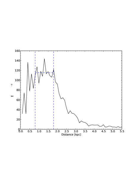
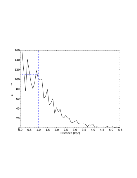
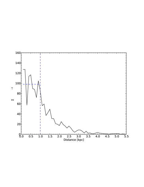
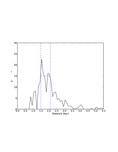
Figure 1: Surface density distribution of clusters as a function of distance in the samples investigated in our work (top-left: CS 1 – Kharchenko; top-right: CS 2 – Dias; bottom-left: CS 3 – WEBDA; bottom-right: CS 4 – FSR). In each panel the vertical dashed line(s) indicate the region where we consider the sample to have a homogeneous completeness and the horizontal dashed line indicates the surface density in this region.

.

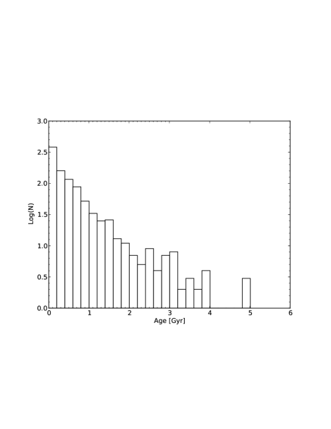
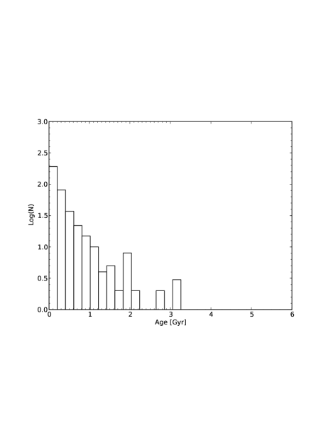
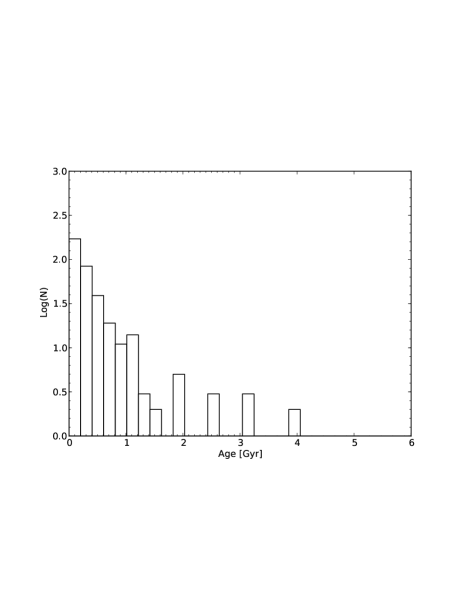
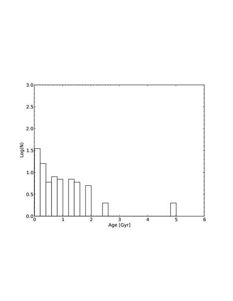
Figure 2: Age distribution of the homogeneously selected cluster sub-samples used in our work (top-left: CS 1 – Kharchenko; top-right: CS 2 – Dias; bottom-left: CS 3 – WEBDA; bottom-right: CS 4 – FSR).

.

3 Isochrone Fitting

For all of the above mentioned cluster samples, except the FSR clusters, there are ages available. To perform our analysis we hence need to determine ages for all the FSR objects. In the following section we detail our approach to fit isochrones with particular emphasis on performing these fits in an unbiased and homogeneous way and to obtain accurate ages.

For each FSR object the most likely cluster members are identified using the established photometric decontamination technique detailed in Paper I (Sect. 3.1). We then fit solar metallicity Geneva (Lejeune & Schaerer, 2001) or pre-main sequence (Siess et al., 2000) isochrones (where appropriate) to the near infrared 2MASS colour-magnitude data of the highest probability cluster members (Sect. 3.2). As starting point we utilise our homogeneously determined distance and extinction values from Paper I. All clusters are then fit three times blindly (without knowledge which cluster is fit) and in a random order. The three values for age, distance and reddening are averaged to obtain the final cluster parameters.

3.1 Cluster Membership Probabilities

To fit isochrones to NIR colour magnitude diagrams of clusters situated along the crowded Galactic Plane, the photometry needs to be decontaminated from foreground and background objects. Otherwise cluster features such as the main sequence and red giant branch are difficult to identify. We have detailed our approach to determine membership probabilities for individual stars in each cluster in Paper I. In the following we just provide a short overview of our method.

The photometric decontamination procedure was originally outlined in Bonatto & Bica (2007) and is based on earlier works by e.g. Bonatto et al. (2004). Froebrich et al. (2010) have slightly adapted the original method to identify cluster members and we have applied the same procedure in Paper I and for the work presented here.

JHK photometry from the 2MASS (Skrutskie et al., 2006) point source catalogue is utilised for all stars in a cluster with a photometry quality flag of Qflag=’AAA’. The radius of the circular cluster area ($A_{cl}$) around the cluster centre is chosen as one or two times the cluster core radius. The control area ($A_{con}$) is a ring with an inner radius of five core radii and an outer radius of $0.5^{\circ}$. We define the Colour-Colour-Magnitude distance, $r_{ccm}$, between the star, $i$, and every other star $j\neq i$ in the cluster area as:

$$r_{ccm}=\sqrt{\frac{1}{2}\left(J_{i}-J_{j}\right)^{2}+\left(JK_{i}-JK_{j}\right)^{2}+\left(JH_{i}-JH_{j}\right)^{2}},$$ (1)

where $JK=J-K$ and $JH=J-H$ are the 2MASS NIR colours. We then determine $r^{N}_{ccm}$ as the distance to the $N^{\rm th}$ nearest neighbour to star $i$ within the cluster area in this Colour-Colour-Magnitude space. As detailed in Paper I, the exact choice of the value for $N$ will not influence the results, i.e. the identification of the most likely cluster members. Thus, in accordance to our procedure in Paper I we set $N=25$. We then count the number of stars ($N^{con}_{ccm}$) in the control field that are closer to star $i$ in the Colour-Colour-Magnitude space than $r^{N}_{ccm}$. Normalising this number by the respective area allows us to determine the membership-likelihood index or cluster membership probability ($P^{i}_{cl}$) of star $i$ via:

$$P^{i}_{cl}=1.0-\frac{N^{con}_{ccm}}{N}\frac{A_{cl}}{A_{con}}.$$ (2)

Should statistical fluctuations lead to negative $P^{i}_{cl}$ values, then the membership probabilities for this particular star are set to zero. Note that we are only interested in the most likely cluster members, whose $P^{i}_{cl}$ values will not be influenced by this.

3.2 Isochrone fitting

Using the above determined cluster membership probabilities for stars in each cluster region, we utilise NIR colour-magnitude and colour-colour diagrams to fit isochrones to the data (see Fig. 3 for an example). Since we have no data available on the metallicities of the clusters, we homogeneously assume solar metal content. This could be not appropriate for particular clusters, whose [Fe/H] might range from -0.4 to +0.2, but statistically this assumption is justified. Furthermore, the median metallicity of all our clusters that have a WEBDA counterpart is $Z=0.02$ (i.e. solar). We also note that our statistical errors of the cluster parameters caused by the manual isochrone fits are typically of the order of, or larger than, the systematic uncertainties caused by using a slightly erroneous metallicity. Furthmore, the age binsize used in our analysis in Sect. 5.2.1 is also of the same size or larger than potential age variations due to variations in the metallicity. Hence, the clusters in each bin provide a statistically valid representation of the age.

As model isochrones we utilise the Geneva Isochrones (Lejeune & Schaerer, 2001) for intermediate age and old clusters. In some cases the clusters are obviously very young, i.e. contain Pre-Main Sequence (PMS) stars. For these objects we utilise the solar metallicity PMS isochrones from Siess et al. (2000) which cover the stellar mass range of ($0.1M_{\odot}<M<7.0M_{\odot}$).

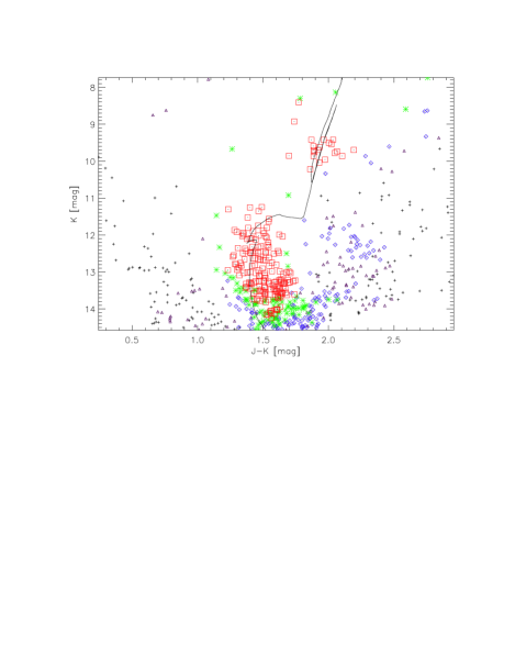
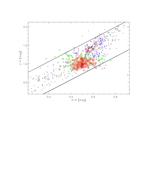
Figure 3: Isochrone fits for all stars within two cluster core radii for FSR 0233. Symbols represent the determined cluster membership probabilities:$P^{i}_{cl}>80$ % red squares; $60\%<P^{i}_{cl}<80$ % green stars; $40\%<P^{i}_{cl}<60$ % blue diamonds; $20\%<P^{i}_{cl}<40$ % purple triangles; $P^{i}_{cl}<20$ % black plus signs. The left panel, shows the isochrone fit in the $J-K/K$ colour magnitude space, the right panel shows the isochrone fit in the $H-K/J-H$ colour colour space. The overplotted isochrone (black solid line) has the parameters of $log(age/yr)=9$, distance of $d=1.6$ kpc and H-band extinction $A_{H}=1.3$ mag.

3.2.1 Unbiased isochrone fits

Our aim is to determine the cluster properties (age, distance, reddening) and uncertainties for all FSR clusters in a homogeneous way. In order to achieve this we set up a manual pipeline which will be described in the following.

We only select FSR cluster candidates for which we have been able to automatically measure distance and reddening in Paper I. These are 771 of the FSR objects. The remaining clusters and cluster candidates will have an insufficient number of high probability cluster members, and hence any attempt to fit an isochrone to these objects will most likely be impossible or result in very large uncertainties.

In the literature there are many examples of a single cluster having multiple determined age, distance and reddening values. One such example is FSR 1716 (as discussed in the introduction) for which Froebrich et al. (2010) determined a distance of 7.0 kpc and $\log(age/yr)$ = 9.3, whereas Bonatto & Bica (2008) determined the cluster to be either 0.8 kpc$/$7 Gyr or 2.3 kpc$/$12 Gyr. A similar case discussed in Sect. 2 is Stephenson 2 (or RSGC 2). This is a young embedded, red supergiant rich cluster at a distance of about 6 kpc (e.g. Davies et al. (2007); Froebrich & Scholz (2013)), while Kharchenko et al. (2013) lists a distance of only 1.13 kpc. Such inconsistencies can arise from different interpretations of which stars are potentially giants in the cluster. To account for these possibilities we decided to fit an isochrone to each cluster three times using a blind fit (the FSR number or previous fit results are unknown) and a randomised order.

Thus, one of us performed 2313 manual isochrone fits. In every case neither the FSR number nor the results from previous fits are known. We start each fit with plotting the NIR colour-magnitude and colour-colour diagrams (as shown in Fig. 3) where stars are coded based on their determined cluster membership probability. Overlayed on these plots are several Geneva isochrones of different ages ($\log(age/yr)$ = 7, 8, 9, 10) using the distances and extinction values for this cluster from Paper I.

The fitter then categorises the cluster in one of three types: i) unable to fit any kind of isochrone; no feature(s) resembling a star cluster is visible in the diagrams, hence the cluster is either not real or the object represents an overdensity that is too low to reliably identify the position of the most likely cluster members in the colour-magnitude diagrams; ii) cluster age identified as young; these objects are then fit by a pre-main sequence isochrone; iii) a clear intermediate age or old open cluster sequence is visible; for these objects the closest fit of the four isochrones is chosen and overlayed with a number of isochrones with steps in $\log(age/yr)=0.05$. The then closest fit is used as a starting point to freely vary all three isochrone parameters (age, distance, reddening) until a satisfactory fit is obtained. A similar procedure is performed for the pre-main sequence clusters.

3.2.2 Cluster characterisation and parameters

Once the entire sample of cluster candidates has been fitted by the above described method, i.e. there are three independent fits and classifications for each candidate, the results for each cluster are combined and objects are classified into the three categories discussed above.

i) A cluster candidate is considered not a cluster or a too low significant overdensity if it has been placed at least twice into this category, or if it has been placed in each of the three categories once.

ii) An object is considered a PMS cluster if it has been placed at least twice into this category.

iii) An object is considered an open cluster if it has been placed at least twice into this category.

For the latter two categories we determine the cluster parameters (distance, age, extinction) as averages from the respective isochrone fits (either three or two). The resulting values are listed in the Appendix in Table LABEL:app_table. The uncertainties listed in Table LABEL:app_table are then the mean absolute statistical variations of the individual parameter values for each cluster as obtained by the fitter. Note that they do not include any systematic uncertainties caused by using solar metallicity isochrones.

4 Scale Height determination

4.1 Cluster distribution functions

In order to analyse the distribution of star clusters perpendicular to the Galactic Plane, one can assume that the space density $N(Z)$ of clusters as a function of the height $Z$ above/below the plane follows a certain analytical function. This could be for example an exponential distribution of the form

$$N(Z)=N_{0}\cdot\exp\left(-\frac{\left|Z-Z_{0}\right|}{h_{0}}\right),$$ (3)

or

$$N(Z)=N_{0}\cdot sech^{2}\left(\frac{\left|Z-Z_{0}\right|}{2\cdot h_{0}}\right),$$ (4)

which is to be expected for a self-gravitating disk. In both equations $N_{0}$ gives the central space density of clusters at $Z=Z_{0}$, where $Z_{0}$ is the vertical centre (zero point) of the distribution and $h_{0}$ is the scale height. Both distributions are very similar within a few scale heights, and are in fact identical at $\left|Z-Z_{0}\right|=h_{0}$.

We plan to investigate the evolution of the scale height $h_{0}$ as a function of cluster age and also the distance of the clusters from the Galactic Centre. The cluster samples we can utilise usually only include objects at most a few scale heights from the mid-plane. It is hence not of relevance which parametrisation we utilise and we chose the exponential distribution for the purpose of this paper.

Furthermore, our sample sizes to determine the free parameters of this distribution ($N_{0},Z_{0},h_{0}$) are going to be small. Hence, any algorithm to determine these parameters needs to be robust for small samples and also allow us to estimate realistic uncertainties for each of the parameters in order to reliably infer trends or to identify differences in e.g. $h_{0}$ which are statistically significant. Note that a simple exponential fit to a histogram for the $Z$ distribution of clusters is not sufficient for this purpose, as it will break down easily even for sample sizes of the order of 100 clusters (see e.g. Bonatto et al. (2006), Piskunov et al. (2006)).

4.2 Parameter determination

In order to ensure reliable values for the parameters ($N_{0},Z_{0},h_{0}$) and accurate uncertainties even for small cluster samples ($N<100$), we compare the distribution of $Z$-values of our sample with model distributions via a two sample Kolmogorow-Smirnov (KS) test (Peacock, 1983). The model distributions are obtained for different scale heights and $Z_{0}$ values. The parameters of our cluster sample are taken as the values of the model distribution which shows the highest probability to be drawn from same parent distribution.

Model Distribution Size

The 2-sample KS-test uses a Cumulative Distribution Function (CDF) for the two samples of $Z$ values to estimate the probability $P_{KS}$ that both are drawn from the same parent distribution. Our model sample of clusters will have to have at least the same range of $Z$-values as the observed sample whose parameters we are trying to determine. With the known $Z_{min}$ and $Z_{max}$ values of the observed sample, in principle we can determine an analytical expression for the CDF of the model by integrating Eq. 3 along $Z$. However, we decided to obtain this CDF by generating a sample of $N_{M}$ $Z$-values randomly distributed according to Eq. 3.

The size of $N_{M}$ should be as small as possible to limit the computing time, but as large as required to remove any uncertainties due to the random nature of the sample. We hence determined $P_{KS}$ values of an observed cluster sample against model cluster samples with $N_{M}$ $Z$-values. The size $N_{M}$ of the model cluster sample was varied from 300 to 50.000 objects. For each $N_{M}$-value we repeated these tests multiple times with different random realisations of the distribution of $Z$-values. The size $N_{M}$ of the model sample was judged to be sufficient when for 9 out of 10 random realisations the $P_{KS}$ were identical. This occurred for model sizes of about $N_{M}=30,000$. Note that we have repeated these tests for multiple combinations of $h_{0}$ and $Z_{0}$ values in the model, with no changes to the results. Hence, all our model cluster samples contain 30,000 clusters.

Model Parameter Ranges

As mentioned above, all our model distributions will contain $Z$-values for 30,000 objects within the minimum and maximum $Z$-value of the observed distribution whose parameters we are trying to determine. We want to determine the parameters ($h_{0},Z_{0}$) of the observed distribution without any prior assumptions. Thus, we generated model distributions where the parameters $h_{0}$ and $Z_{0}$ did span the entire possible parameter space. In other words we varied $h_{0}$ between 20 pc and 1000 pc, while $Z_{0}$ had values between -160 pc and +100 pc. In both cases 5 pc increments where chosen for both parameters. This resulted in 197 x 53 = 10,441 different model distributions for each of the observed cluster samples.

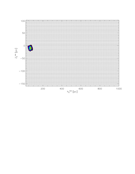
Figure 4: Plot of the $P_{KS}$ values for an observed cluster distribution for the entire modelled $h_{0}$ vs $Z_{0}$ parameter space. Crosses indicate the positions for which we performed a KS-test. The colours/contours indicate the probabilities that the modelled and observed distributions are drawn from the same parent sample. Most of the $P_{KS}$ values are almost zero (white, lowest contours), and the highest non-zero values (red, highest contours) are only found in a small area of the parameter space. The sample contains all clusters from the MWSC catalogue (CS 1) within our chosen distance range in the 4th Galactic quadrant. There are 313 clusters in this sample and we find a best fit for the scale height of 68.1 pc and the vertical zero point of -9.9 pc.

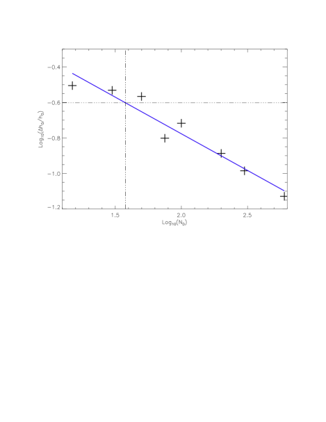
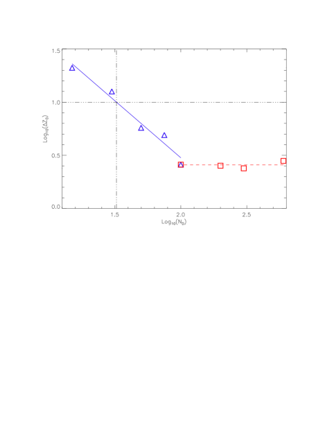
Figure 5: Left: Plot of scale height relative error against sample size. Black crosses represent the mean values for the modelled distributions. The solid line represents our fitted power law, and the dot-dash lines a 25 % error on the scale height, which is achieved for a sample size of 38 clusters or above. Right: Plot of vertical zero point absolute error against sample size. Blue triangles and red squares represent the mean values obtained for the modelled distribution. The blue solid line and red dashed line represent the respective linear fits to sample sizes below and above 100 clusters. The dot-dash lines identifies an error of 10 pc for $Z_{0}$ which is achieved for a sample size of 32 clusters or larger.

Best Fit Parameters

We now perform a 2-sample KS-test of the observed sample against all the 10,441 model distributions to determine the probabilities $P_{KS}$ that the two samples are drawn from the same parent distribution. In Fig. 4 we show the distribution of $P_{KS}$-values for one example of an observed cluster distribution (all selected clusters from CS 1 in the 4th Galactic Quadrant) over the entire modelled $h_{0}$–$Z_{0}$ parameter space, i.e. the figure shows $P_{KS}(h_{0},Z_{0})$. As one can see, for vast regions of the parameter space, the $P_{KS}$-values are almost zero. Only for a limited area the the values are non-zero.

In order to find the best fitting parameters for the observed distribution we do not chose the set of parameters that leads to the highest probabilities $P_{KS}$. Instead we fit a 2-dimensional Gaussian distribution to the $P_{KS}(h_{0},Z_{0})$ values, where the centre and width are free parameters. The central coordinates of this Gaussian are then taken as the best fit parameters for the observed distribution.

4.3 Parameter Uncertainties

Our above described approach generates two best-fit parameters for each observed cluster distribution. Since we plan to investigate potential changes with age or Galactocentric distance of the scale height of our observed cluster distributions, we require to know the uncertainties of our method in order to judge if any trends in the data are significant. In other words we need to estimate how large the uncertainties $\Delta h_{0}$ and $\Delta Z_{0}$ are and if/how these uncertainties depend on the value of the parameters and the size of the cluster sample.

In order to estimate these uncertainties we simulated $Z$-distributions for small cluster samples with various $h_{0}$ and $Z_{0}$ values and processed them with our above described procedure to determine their scale height and vertical zero point. Since we know the input parameters for each simulated distribution, we can evaluate the uncertainty for both parameters by repeating the process with 50 different random realisations of the simulated $Z$-distributions. The uncertainties $\Delta h_{0}$ and $\Delta Z_{0}$ are estimated as the $rms$ of the individual measurements $h_{0,i}$ and $Z_{0,i}$ compared to the input values.

To test any dependencies of the uncertainties on the parameter values of $h_{0}$ and $Z_{0}$ we did two tests: i) we kept $Z_{0}$ = -30 pc and varied $h_{0}$ between 100 pc and 350 pc, which covers the potential range of scale heights for most of our observed samples; ii) we fixed the scale height to $h_{0}$ = 200 pc and varied the vertical zero point of the distribution from -40 pc to +40 pc. In both cases no significant or systematic dependence of the uncertainties on the parameter values is found.

More importantly, we also need to test how the uncertainties depend on the sample size $N_{D}$. We hence repeated all the above tests for simulated cluster samples with $N_{D}$ = 15, 30, 50, 75, 100, 200, 300 and 600 clusters. We find that the sample size $N_{D}$ has a systematic and significant influence on the uncertainties of both parameters $h_{0}$ and $Z_{0}$. In particular we find that the relative uncertainty of the scale height scales with the sample size $N_{D}$ approximately as a power law. Also the absolute uncertainty of the vertical zero point of the distribution scales as an approximate powerlaw with the sample size, but only for small samples. Above a sample size of about 100 clusters, the absolute uncertainty of $Z_{0}$ remains constant. This is shown in Fig. 5.

From our powerlaw fits we can hence calculate the uncertainties from our method solely from the knowledge of the sample size $N_{D}$ using the following equations:

$$\frac{\Delta h_{0}}{h_{0}}=1.12\cdot\left(N_{D}\right)^{-0.41}$$ (5)

$$\Delta Z_{0}=\left\{\begin{array}[]{l l}419\,\text{pc}\cdot\left(N_{D}\right)^{-1.07}&\quad\text{if $N_{D}<115$}\\ 2.6\,\text{pc}&\quad\text{if $N_{D}>115$}\end{array}\right.$$ (6)

In other words, the relative uncertainty of the scale height scales roughly with the inverse of the square root of the sample size, while the absolute uncertainty of the zero point scales as the inverse of the sample size. We believe that the constant uncertainty of the zero point $Z_{0}$ above a sample size of about 100 clusters is caused by our step size of 5 pc in the model distributions. For such large samples the uncertainty becomes smaller than half of our step size, which then becomes the limiting factor compared to the sample size. Should higher accuracies for $Z_{0}$ be required, the step size can be decreased. We refrain from this in this paper, since we judge 2.6 pc as uncertainty for $Z_{0}$ for large samples sufficient.

5 Results and Discussion

5.1 FSR cluster characterisation and parameters

Our data-processing pipeline was applied to the sub-sample of 775 FSR List clusters which had a distance and extinction values determined in Paper I. Here we successfully determine the ages of 298 clusters. All their parameters and respective uncertainties are listed in the Appendix in Table LABEL:app_table. Hence, only about 40 % of the investigated FSR clusters passed our stringent criteria for a successful isochrone fit. Of those, 216 are flagged as previously ’known’, and 82 as ’new’ in the FSR catalogue. Note, that ’new’ stands for clusters that are new discoveries in (Froebrich et al., 2007). Thus, we confirm here that these 82 previously unknown objects are in fact real clusters and determine their parameters.

The low percentage of these ’new’ clusters in the entire sample can be interpreted in two ways: (i) A large fraction of these clusters are overdensities but not in fact real clusters, i.e. no isochrone could be fitted; (ii) It is significantly more difficult to fit isochrones to these clusters since they are less significant overdensities.

Froebrich et al. (2007) showed that about half of the entire FSR list of ’new’ objects might in fact be not real clusters but overdensities, which was confirmed through spatial analysis by Bica et al. (2008) and Camargo et al. (2010). However, as discussed in Paper I, the contamination of the cluster sub-sample of 775 objects used here is less than 25 %, thus at least 75 % of the clusters are potentially real. During the isochrone fits for the clusters in our FSR sub-sample, it was noted that a large proportion of clusters had a poorly defined main sequence; in many cases only the top was visible within the 2MASS magnitude limit and thus an isochrone fit was not possible under the constraints of our data-processing pipeline. On completion of the pipeline, we found that a large proportion of the known objects had a clear and well defined main sequence and$/$or red giants, whereas the unknown objects had fewer members (hence they remained undetected) whose main sequences were not as well defined, and in many cases fell below the magnitude limit of 2MASS. We would argue, therefore, that the low number of confirmed new clusters in our sample is a reflection of the difficulty involved in fitting isochrones to the new objects, rather than the majority being over-densities.

We make a comparison of the distance and H-band reddening values determined in Paper I using our novel photometric method ($D^{PI},A_{H}^{PI}$), and those from our data-processing pipeline described in Sect 3.2.2 of this paper ($D^{P2},A_{H}^{P2}$). The two distance values depend linearly on one another, with $D^{P1}\approx 25\%$ larger than $D^{P2}$, with a scatter of 65 % and Pearson correlation coefficient of 0.89. The primary source of the large scatter are clusters concentrated at small distances, i.e. $D^{P2}\leq 3kpc$. The scatter decreases with increasing $D^{P2}$. This can be explained since our photometric distance measurement method in Paper I works by measuring the density of stars foreground to a cluster which is more accurate for larger, more extincted objects.

The two reddening values also depend linearly on one another, agreeing within $5\%$ with a scatter of $9\%$ and Pearson correlation coefficient of $0.95$. Unlike $D^{P1}$, the determination $A_{H}^{P1}$ depends only on the ability to accurately determine a clusters median colour, and hence is independent of individual cluster reddening values.

Furthermore, we have compared our ages to the ages in MWSC, for the clusters which are in both lists. There are a few obvious outliers, where ages differ by a factor of 10 or more. However, after removing those, both ages show a correlation coefficient of 0.73, with a rms scatter of 0.19 for log(age/yr). The latter can be interpreted as a more realistic uncertainty of the ages determined for the FSR clusters, compared to the pure statistical estimates quoted in Table LABEL:app_table.

As already stated in Sect. 2, the resulting FSR sub sample after the age determination is only very small. If we further require a homogeneous completeness for the scale height analysis, the sample size becomes even smaller. Hence we have not included the FSR-subsample in the scale height analysis performed in the remainder of the paper. However, as is evident in the radial distribution (lower right panel of Fig. 1) and the age distribution (lower tight panel of Fig. 2) sample is dominated by rather old, and distant clusters. They are hence in itself an important addition to the existing large cluster samples, potentially enlarging their current radius of completeness.

5.2 Cluster Scale Height and Zero Point

Our novel method is designed to determine a cluster sample’s scale height $h_{0}$ and zero point $Z_{0}$, whilst significantly reducing the restraint on sample size. The approach to utilise modelled distributions in conjunction with KS-tests allows us to determine $h_{0}$ with a better than 25 % accuracy for a sample of 38 clusters or larger. For the same sample size we can determine $Z_{0}$ within 8.5 pc. In the following we hence investigate sub-samples of CS 1, 2, 3 with roughly this size, in order to establish if there are systematic and/or significant evolutionary or positional trends in the cluster distribution within the plane of the Galaxy. We investigate each of the three cluster samples to find out if there are differences between them that might be caused by potential biases in the samples.

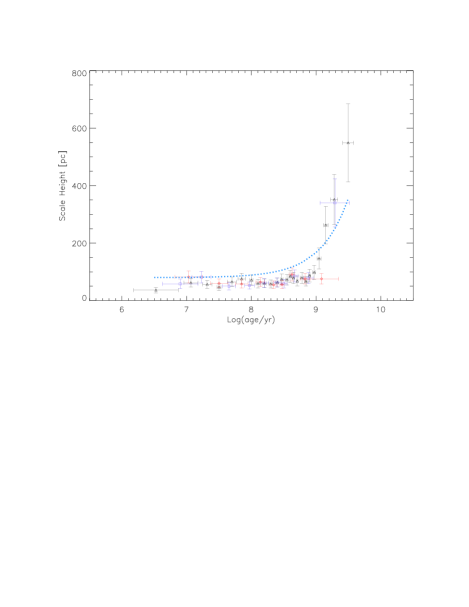
Figure 6: Evolution of the cluster scale height $h_{0}$ with age for the 3 investigated samples. Black triangles indicate CS 1 (MWSC), blue squares indicate CS 2 (DAML02) and red diamonds CS 3 (WEBDA). The horizontal ’age’ error bars indicate the typical rms of log(age/yr) from the median age in each bin. The dashed line is the approximate scale height – age relation for field stars (see text for details).

5.2.1 $h_{0}$ Evolution with Age

We investigate how scale height changes with cluster age. In Fig 6 we show the scale height values we derived using our method over a range of age bins. The age ranges for each bin and the number of clusters in them for every CS are listed in Table 1. There is a general trend of increasing scale height with cluster age. Most notably there is an apparent marked increase in the gradient at $log(age/yr)=9$ or a cluster age of about 1 Gyr. We perform a linear fit of the scale height against $log(age/yr)$ and find that the observational trend in Fig. 6 can be characterised by:

$$h_{0}\propto\left\{\begin{array}[]{rl}11.0\,\text{pc}\cdot log(age/yr)&\quad\text{if age $\leq$ 1\,Gyr}\\ 880\,\text{pc}\cdot log(age/yr)&\quad\text{if age $\geq$ 1\,Gyr}\end{array}\right.$$ (7)

where $h_{0}$ is the scale height and $log(age/yr)$ is the cluster age. Note that at an age of 10 Myr, the time when gas expulsion has typically finished, the scale height of the clusters is about 50 pc. Please note that the above given values for the changes of scale height with cluster age are independent of the actual choice of the borders for our age bins. The only sample where the marked change in behaviour at 1 Gyr is not evident is CS 3 – WEBDA. The reason is that in our homogeneously selected sub-sample there are simply not enough old clusters to trace $h_{0}$. In particular the oldest age bin spans a factor of 14 in age (see Table 1), but is dominated by clusters of an age of 1 Gyr. CS 1 and CS 2 show essentially the same behaviour for older objects (see Fig. 6), even if there is just one ’old’ age bin for CS 2.

Table 1: Age bins (minimum and maximum ages) and respective number of clusters in them for the clusters samples, used in the investigation of scale height with cluster age. We also list the determined scale height and zero point with their respective uncertainties.

CS	Agemin	Agemax	Ncl	$Z_{0}$	$\Delta Z_{0}$	$h_{0}$	$\Delta h_{0}$
	[log(age/yr)]			[pc]		[pc]
MWSC	6.000	6.850	40	-2	8	36	9
MWSC	6.850	7.200	40	9	8	62	15
MWSC	7.200	7.420	40	6	8	56	14
MWSC	7.420	7.550	40	-20	8	47	12
MWSC	7.550	7.755	40	-10	8	65	16
MWSC	7.760	7.950	40	-6	8	76	19
MWSC	7.950	8.060	40	-20	8	72	18
MWSC	8.060	8.150	40	-3	8	59	15
MWSC	8.150	8.255	40	-1	8	60	15
MWSC	8.255	8.350	40	-9	8	58	14
MWSC	8.350	8.445	40	-13	8	63	16
MWSC	8.445	8.505	40	-22	8	74	18
MWSC	8.505	8.580	40	-9	8	73	18
MWSC	8.585	8.632	40	-24	8	85	21
MWSC	8.635	8.690	40	-29	8	79	20
MWSC	8.695	8.735	40	-8	8	68	17
MWSC	8.735	8.800	40	-25	8	79	20
MWSC	8.800	8.865	40	-12	8	67	16
MWSC	8.870	8.930	40	-9	8	87	21
MWSC	8.935	9.005	40	-23	8	98	24
MWSC	9.005	9.100	40	-39	8	146	36
MWSC	9.100	9.200	40	8	8	263	65
MWSC	9.200	9.400	40	-109	8	352	87
MWSC	9.400	9.700	40	-56	8	549	135
DAML02	6.00	7.02	29	-35	11	58	16
DAML02	7.03	7.50	40	-41	8	82	20
DAML02	7.50	7.83	40	-25	8	50	12
DAML02	7.84	8.09	40	-13	8	53	13
DAML02	8.09	8.30	40	-16	8	61	15
DAML02	8.30	8.45	40	-13	8	63	16
DAML02	8.45	8.60	40	11	8	59	15
DAML02	8.60	8.78	40	-23	8	86	21
DAML02	8.78	9.01	40	-13	8	78	19
DAML02	9.03	9.90	40	-20	8	340	84
WEBDA	6.00	7.17	38	-51	9	82	21
WEBDA	7.20	7.66	40	-25	8	60	15
WEBDA	7.68	8.00	40	-23	8	58	14
WEBDA	8.00	8.23	40	-4	8	64	16
WEBDA	8.23	8.42	40	-26	8	55	14
WEBDA	8.42	8.54	40	5	8	56	14
WEBDA	8.55	8.69	40	-21	8	91	22
WEBDA	8.69	8.95	40	-34	8	76	19
WEBDA	8.96	10.12	40	-9	8	76	19

Previous efforts to determine the $h_{0}$ of older clusters as a function of age have had limited success. Restrictions on sample size caused by the small size of the older cluster sample and the spread of their distributions with increasing age, has until now prevented a detailed analysis of evolution of the scale height of old clusters. Attempts to place a value on the scale height have yielded a value of $h_{0}=375pc$ for clusters older than 1 Gyr (e.g. Froebrich et al. (2010)). From Eq. 7 and Fig. 6, this value corresponds to an age of about 2.2 Gyr i.e. in the middle of the ’old’ cluster age bin. Hence this literature value is an average scale height for clusters older than 1 Gyr. Figure 6 also demonstrates the superiority of the MWSC list in combination with our novel approach to determine the scale height, as the larger sample size of CS 1 allows us to clearly trace the scale height evolution for objects older than 1 Gyr in several bins and to show that there is a systematic significant observational trend in the cluster scale height with age for objects up to 5 Gyr.

To the best of our knowledge there are currently no numerical investigations of the scale height of stellar clusters as a function of age in the Galactic Plane. This is most likely due to the complexity of the problem which requires following the evolution of individual stars in clusters of varying mass to account for the cluster dissolution over time, as well as the cluster as a whole in the gravitational potential of the Galactic Disk. However, we can try to compare the scale heights of objects of different ages with the here determined evolution of $h_{0}$ for clusters to infer the basic physical reasons for the evolution, and in particular the marked change in behaviour after about 1 Gyr.

The dust in the Galactic Plane has a scale height of about 125 pc (Drimmel et al., 2003; Marshall et al., 2006) in the vicinity of the Sun. At an age of 1 Myr, Fig. 6 and Eq. 7 show that young star clusters have a scale height of 40 pc. This is right in the middle of the range of scale heights estimated for massive OB-stars (30 – 50 pc; (Reed, 2000; Elias et al., 2006)). Since the formation of these massive stars is inextricably linked to clustered star formation, this is expected. Thus, the formation of massive stars and clusters is only possible within the densest part of the ISM (within one third of the dust scale height), and no significant fraction of locally observable clusters (without OB-stars) forms in lower density environments, further away from the disk midplane.

The number of clusters declines over time (see Fig. 2) which is well known and understood from numerical models (e.g. Gieles et al. (2008); Gieles (2009); Lamers & Gieles (2006); Lamers et al. (2005)). Causes of disruption timescales depend on both internal and external processes such as e.g. stellar evolution, tidal stripping and relaxation, shocking by spiral arms and encounters with giant molecular clouds. A consensus in the literature has not yet been reached on the role that cluster mass plays in disruption (for a discussion see e.g. Bastian (2011)). The dominant disruption process at a few 100 Myr is stellar evolution through member loss. In combination with external processes, clusters may gain enough energy from the ejection of low mass members to cause the observed moderate changes in scale height during that phase. We find a 10 pc increase in $h_{0}$ per $dex$ in cluster age from the formation to 1 Gyr, but the correlation coefficient is only 0.5, and as low as 0.1 when only considering the first 300 Myr of evolution. Thus for the first few 100 Myr the data suggest no evolution in $h_{0}$, but the scale height at an age of about 1 Gyr reaches about 75 pc. This is comparable or smaller than the scale height of other young objects in the disk (e.g. 130 pc for bipolar PNs (Corradi & Schwarz, 1995); 55 – 120 pc for young WDs (Wegg & Phinney, 2012))

After the surviving clusters reach an age of about 1 Gyr, or a scale height of 75 pc, there is an apparent sudden increase in $h_{0}$ corresponding to a change in the evolutionary behaviour. The increase in scale height is about 880 pc/$dex$ in age. It has been shown that, assuming mass dependent disruption, clusters with a mass of less than $10^{4}M_{\odot}$ and within 1 kpc of the Sun are disrupted after 1 Gyr (Boutloukos & Lamers, 2003). Hence, we expect the cluster sub-samples after 1 Gyr to be dominated by initially massive clusters. Thus, if clusters have survived for this duration, they must have been scattered into an orbit which places them preferentially far away from the Galactic mid-plane. This enables them to spend much less time in the denser parts of the Galactic Disk, decreasing their probability for disruption via external process (spiral arms, encounters with GMCs) and increasing their chances of prolonged survival. In other words, the increase in scale height also implies that the population of old clusters is dominated by objects that have undergone at least one violent interaction event in their past that has moved them into an orbit inclined to the Galactic Plane. This observational evidence should hence be able to put tighter constraints onto comprehensive numerical models of cluster evolution and disruption in the context of the entire Galactic Disk.

Note that the behaviour of the scale height for clusters is markedly different to estimates for field stars. To illustrate this we have overplotted the principle trend observed for main sequence field stars of varying ages in Fig. 6. This qualitative trend has been obtained by utilising colour dependent velocity dispersions for main sequence stars presented in Dehnen & Binney (1998). As one can see in Fig. 6, the heating of the stellar compontent of the disk occurs gradually, while for the cluster component there is a discontinuity around 1 Gyr. This demonstrates the difference of the underlying physical mechanisms for the increase in scale height. While the stellar component is heated via N-body interactions, the tidal field and GMCs, the clusters have a much stronger rate of disappearing from the observational sample with increasing age, and are only moved to large scale heights (and thus able to survive) via interactions with massive objects such as GMCs.

5.2.2 $h_{0}$ Dependence on Galactic Position

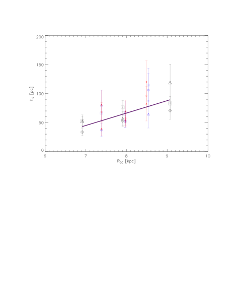
Figure 7: Cluster scale height as a function of galactocentric distance. The symbols indicate different age ranges. Diamonds indicate clusters younger than 80 Myr, triangles indicate clusters with ages between 80 Myr and 200 Myr and squares indicate clusters with ages between 200 Myr and 1 Gyr. Furthermore, the different CSs are indicated by different colours and symbol sizes; large black, medium blue, small red for CS 1, 2, 3, respectively.

Table 2: Age and galactocentric distance ranges used in the investigation of the dependence of scale height on the galactocentric distance. We list the cluster sample, age range, $R_{GC}$ range as well as the determined scale height and zero point with their respective uncertainties. Age bin 1 corresponds to ages less than 80 Myr, age bin 2 corresponds to ages between 80 Myr and 200 Myr and age bin 3 corresponds to ages between 200 Myr and 1 Gyr. Older clusters are not included due to the paucity of these objects.

CS	Age bin	$R_{GC}$	Ncl	$h_{0}$	$\Delta h_{0}$	$Z_{0}$	$\Delta Z_{0}$
		[kpc]		[pc]		[pc]
MWSC	1	6.9 $\pm$ 0.6	90	34	6	-13	3.4
MWSC	1	7.9 $\pm$ 0.7	82	53	10	13	3.8
MWSC	1	9.1 $\pm$ 0.7	60	71	15	-9	5.2
MWSC	2	6.9 $\pm$ 0.6	60	52	11	-4	5.2
MWSC	2	7.9 $\pm$ 0.7	57	57	12	-4	5.5
MWSC	2	9.1 $\pm$ 0.7	33	119	32	2	9.9
MWSC	3	6.9 $\pm$ 0.6	121	53	8	-8	2.6
MWSC	3	7.9 $\pm$ 0.7	134	76	11	-17	2.6
MWSC	3	9.1 $\pm$ 0.7	151	83	12	-23	2.6
DAML02	1	7.4 $\pm$ 0.4	23	37	12	-37	15
DAML02	1	8.0 $\pm$ 0.3	66	52	11	-13	4.7
DAML02	1	8.6 $\pm$ 0.3	33	106	28	-49	9.9
DAML02	2	7.4 $\pm$ 0.4	21	80	26	-4	16
DAML02	2	8.0 $\pm$ 0.3	32	69	19	-21	10
DAML02	2	8.5 $\pm$ 0.3	15	64	24	-26	23
DAML02	3	7.4 $\pm$ 0.4	45	66	16	-14	7.1
DAML02	3	8.0 $\pm$ 0.3	68	52	10	-4	4.6
DAML02	3	8.5 $\pm$ 0.3	38	115	29	-17	8.5
WEBDA	1	7.4 $\pm$ 0.4	23	39	12	-41	15
WEBDA	1	8.0 $\pm$ 0.3	59	54	11	-21	5.3
WEBDA	1	8.5 $\pm$ 0.3	24	120	37	-72	14
WEBDA	2	7.4 $\pm$ 0.4	21	80	26	-5	16
WEBDA	2	8.0 $\pm$ 0.3	28	69	20	-13	12
WEBDA	2	8.5 $\pm$ 0.3	16	82	30	-36	22
WEBDA	3	7.4 $\pm$ 0.4	44	68	16	-14	7.3
WEBDA	3	8.0 $\pm$ 0.3	64	57	12	-17	4.9
WEBDA	3	8.5 $\pm$ 0.3	42	96	23	-10	7.7

We investigate if the cluster scale height changes with Galactocentric radius, $R_{GC}$. To eliminate the apparent age effects discussed in Sect. 5.2.1, we determine $h_{0}$ for 4 age bins. These are: bin 1 – age less than 80 Myr; bin 2 – age between 80 Myr and 200 Myr; bin 3 – age between 200 Myr and 1 Gyr; bin 4 – age above 1 Gyr. Each of these age bins is separated into 3 ranges for the $R_{GC}$ values per cluster sample. See Table 2 for details of each bin. Note that this table does not contain the details for the oldest age bin 4, as the paucity of old clusters did not allow to split them into several $R_{GC}$ bins and still being able to determine scale height and zero point with sufficient accuracy to draw any meaningful conclusions. In Fig. 7 we show that there is a positive trend between $h_{0}$ and $R_{GC}$ for clusters younger than 1 Gyr, which can be expressed as:

$$h_{0}[pc]\propto 0.02\cdot R_{GC}[pc]$$ (8)

where $h_{0}$ is scale height and $R_{gc}$ is the median Galactocentric distance of a cluster sample. There is considerable scatter, but the Pearson Correlation Coefficient for the data points, determined including the uncertainties, ranges from 0.75 to 0.85 for the age bins 1 – 3. It has a value of 0.80 for the combined sample of all three age bins shown in Fig. 7. The trend of increasing scale height with $R_{gc}$ is virtually identical for the age bins 2 and 3, and only slightly stronger for the youngest clusters in bin 1. Note that at the solar distance to the Galactic Centre (assumed to be 8 kpc) the clusters have a scale height of about 65 pc.

For some of the above not considered $R_{GC}$ bins of the old clusters (age above 1 Gyr), we where able to determine the scale height. The values for $h_{0}$ are dominated by the younger clusters in the age bin, and all scale heights are between 200 pc and 400 pc. However, no correlation of the scale height with $R_{GC}$ is evident for these older clusters. This is expected from our findings in the last section, which indicated that the old objects are dominated by clusters scattered away from the plane in the past.

As for the age evolution of the scale height, there are to the best of our knowledge no numerical simulations to investigate this. Hence, our data should proof vital to constrain potential large scale numerical simulations of cluster evolution in the Galactic Disk. However, we can try to understand this weak observed trend to infer its cause. Since we have eliminated the effect of cluster age, by considering the different age bins, and have found that there is almost no evolution of $h_{0}$ for the first few 100 Myr, any trend in the scale height of the cluster sample has to be imprinted on it during the formation. Indeed there seems to be a moderate flaring of the molecular (star forming) material in the disk (e.g. Sanders et al. (1984); Wouterloot et al. (1990)). More massive clusters (which include OB-stars) should also form closer to the mid-plane. These are the objects which are more likely to survive for a given time. Thus, potentially the observed effect could be caused by the fact that at smaller $R_{GC}$ values there are more massive clusters formed, originally closer to the mid-plane, than further out at larger $R_{GC}$. Hence the scale height is dominated by originally higher mass clusters towards low $R_{GC}$ and by less massive clusters at higher $R_{GC}$. However, only detailed numerical simulations of cluster populations in the Milky Way in combination with accurate cluster mass estimates, both outside the scope of this work, can investigate this properly. Note that this weak trend could in part also be explained by a systematic metallicity gradient in the Galactic Disk.

5.2.3 Vertical Displacement $Z_{0}$

We also investigate how $Z_{0}$ changes with cluster age and $R_{GC}$. We find that there is no dependency of $Z_{0}$ with any of the parameters for our samples. This is an expected result as the spatial distribution of clusters should follow the symmetrical distribution function for vertical displacement above/below the Galactic plane (Eq. 3, 4), such that cluster interactions and disruptions are also symmetrical. Thus, as $h_{0}$ increases with cluster age, $Z_{0}$ will remain constant and only depend on the position of the Sun with respect o the plane.

We have used this to average all the $Z_{0}$ values in our samples to obtain the mean vertical displacement of the Sun with respect to the Galactic Plane based on the local distribution of stellar clusters. We find a mean value of $Z_{0}=-18.5\pm 1.2pc$, and thus $Z_{\odot}=18.5\pm 1.2pc$ (which is in agreement with accepted literature values based on other objects, see e.g. Reed (2006), Humphreys & Larsen (1995)).

6 Conclusions

We aim to study the temporal and spatial evolution of the scale height of star clusters in the Galactic Plane.

In a first step we successfully determined ages of 298 clusters from the FSR list by (Froebrich et al., 2007) by fitting isochrones. We used our automatically determined distances and reddening values from Buckner & Froebrich (2013) as starting points. Our FSR sub-sample is dominated by old objects (age $>$ 500 Myr) with distances between 1.5 kpc and 2 kpc. The distances and extinction values obtained by the isochrone fitting and our purely automatic method based on NIR photometry (Buckner & Froebrich, 2013) show a good correlation with Pearson Correlation Coefficients of 0.89 and 0.95, respectively.

We have developed a novel method to determine the scale height and vertical zero point of cluster distributions using models and Kolmogorow-Smirnov tests. This significantly lessens the restraint on the sample size and allows us to measure scale heights with 25 % accuracy for cluster samples as small as 38 objects. At the same time we are able to infer the sample zero point within 8.5 pc. For larger samples these errors can be significantly reduced.

To investigate the temporal evolution of cluster scale height we investigated homogeneously selected sub-samples of star clusters from four large star cluster catalogues (MWSC (Kharchenko et al., 2013), DAML02 (Dias et al., 2002), WEBDA, FSR (Froebrich et al., 2007)). The selected sub-sample of the FSR list is too small to be included in our subsequent analysis. We find that most of our results are independent of the cluster catalogue, despite their very different criteria for cluster inclusion and parameter estimation. As expected, the MWSC catalogue in combination with our novel scale height determination method, provides the best ’time resolution’ for our investigation.

We find that star clusters are formed (age 1 Myr) with a scale height of 40 pc. This is the same as what has been found for OB-stars (Reed, 2000; Elias et al., 2006), demonstrating the link of massive and clustered star formation. For the next 1 Gyr the scale height of the surviving clusters only marginally increases by about 10 pc per $dex$ in age until it reaches about 75 pc. The data are in agreement with no evolution of $h_{0}$ for the first few 100 Myr.

Fom 1 Gyr onwards the scale height of the surviving cluster population increases significantly faster with about 880 pc per $dex$ in age. The reason for this is most likely that the old cluster sample is dominated by objects which have been scattered by one or more interactions with Giant Molecular Clouds into orbits away from the Galactic Plane. Clusters that do not undergo such a violent event will stay close to the plane, and not survive to ages of several Gyr. This is markedly different to the behaviour of the stellar component in the Galactic Disk.

We further find a weak age-independent trend of cluster scale height with distance from the Galactic Centre. This might be caused by the mass dependence of the formation of stellar clusters in the disk or a metallicity gradient. No significant temporal or spatial variations of the zero point of the cluster distribution have been found. Based on the cluster distribution we estimate that the Sun has a position of 18.5 $\pm$ 1.2 pc above the Galactic Plane, in agreement with past measurements using different tracers.

A detailed understanding of the here presented observational evidence can however only be achieved with numerical simulations of the evolution of cluster samples in the Galactic Disk. Furthermore, more accurate observational cluster parameters, such as distances from GAIA, larger complete samples of clusters, as well as accurate mass estimates for them will certainly aid our understanding of how the dissolution of clusters over time contributes to the stellar content of the thin and thick disk of the Galaxy.

Appendix A FSR Cluster Property Table

Table 3: Summary table of the FSR cluster properties determined with our isochrone-fitting pipeline (the full table will be published online only). The table lists the FSR ID number, the cluster type (known open cluster or new cluster candidate), cluster class (PMS or OC), the distance in kiloparsec determined using our photometric method in Paper I ($D^{P1}$), our pipeline ($D^{P2}$) and uncertainty ($\Delta D^{P2}$); the $H$-band extinction values calculated from $H-K$ excess using our photometric method in Paper I ($A_{H}^{P1}$), our pipeline ($A_{H}^{P2}$) and uncertainty ($\Delta A_{H}^{P2}$); the age in $\log(age/yr)$ and uncertainty ($\Delta\log(age/yr)$). Note that $\Delta A_{H}^{P2}$ and $\Delta\log(age/yr)$ are only the statistical variations of the three isochrone fits and do not account for systematical uncertainties due to the use of solar metallicity isochrones.

FSR	Type	Class	l	b	$D^{P1}$	$D^{P2}$	$\Delta D^{P2}$	$A_{H}^{P1}$	$A_{H}^{P2}$	$\Delta A_{H}^{P2}$	Age	$\Delta$Age
ID			[deg]	[deg]	[kpc]	[kpc]	[kpc]	[mag]	[mag]	[mag]	[$\log(age/yr)$]	[$\log(age/yr)$]
0032	Known	OC	9.28	-2.53	2.8	1.70	0.00	0.21	0.22	0.00	9.10	0.00
0045	Known	OC	12.87	-1.32	2.2	2.60	0.00	0.20	0.32	0.00	8.50	0.00
0071	Known	OC	23.89	-2.91	1.9	2.00	0.21	0.21	0.29	0.02	7.60	0.17
0074	Known	OC	25.36	-4.31	3.5	5.30	0.00	0.18	0.02	0.00	9.50	0.00
0082	Known	OC	27.31	-2.77	1.1	1.60	0.07	0.09	0.14	0.03	8.60	0.09
0089	New	OC	29.49	-0.98	4.5	6.50	0.07	1.53	1.50	0.00	8.50	0.03
0101	New	OC	35.15	1.75	3.2	1.60	0.00	1.07	1.05	0.00	9.20	0.00
0109	Known	OC	37.17	2.62	1.7	1.50	0.03	0.52	0.59	0.01	9.00	0.00
0111	Known	OC	38.66	-1.64	2.0	1.80	0.00	0.19	0.30	0.00	8.80	0.00
0113	Known	OC	39.10	-1.68	1.6	2.10	0.07	0.29	0.39	0.04	8.60	0.18
0115	Known	OC	40.35	-0.70	2.4	2.20	0.00	0.80	1.10	0.00	7.10	0.00
0122	Known	OC	45.70	-0.12	2.1	2.30	0.30	0.64	0.74	0.02	8.60	0.12
0124	New	OC	46.48	2.65	3.7	1.10	0.00	0.48	0.45	0.00	9.30	0.00
0127	Known	OC	48.89	-0.94	2.6	2.90	0.18	0.60	0.64	0.01	8.20	0.02
0133	New	OC	51.12	-1.17	4.2	2.40	0.18	0.87	0.99	0.03	8.70	0.09
0138	Known	OC	53.22	3.34	2.5	3.10	0.07	0.36	0.41	0.01	9.10	0.09
0144	Known	OC	56.34	-4.69	1.9	1.70	0.20	0.02	0.05	0.03	7.80	0.10
0154	New	OC	60.00	-1.08	3.2	3.90	0.00	0.54	0.55	0.00	8.60	0.13
0157	New	OC	62.02	-0.70	2.2	1.10	0.00	0.58	0.65	0.00	6.80	0.00
0167	New	OC	65.16	-2.41	2.4	1.60	0.15	0.42	0.43	0.03	8.70	0.12
0168	Known	OC	65.53	-3.97	1.4	1.00	0.05	0.09	0.09	0.00	8.60	0.03
0169	Known	PMS	65.69	1.18	2.5	2.40	0.00	0.08	0.36	0.00	7.60	0.00
0177	Known	OC	67.64	0.85	3.1	2.80	0.00	0.15	0.30	0.00	9.20	0.00
0186	Known	OC	69.97	10.91	2.0	4.10	0.00	0.25	0.12	0.00	9.50	0.00
0187	Known	OC	70.31	1.76	4.5	5.20	0.00	0.34	0.29	0.00	8.70	0.00
0188	New	OC	70.65	1.74	8.3	10.50	1.00	0.69	0.62	0.02	8.60	0.05
0190	New	OC	70.73	0.96	10.2	11.60	0.00	1.31	1.26	0.00	8.80	0.00
0191	New	OC	70.99	2.58	3.8	2.40	0.37	0.56	0.59	0.04	8.50	0.18
0195	New	PMS	72.07	-0.99	4.1	1.90	0.00	0.99	1.15	0.00	7.60	0.00
0197	New	OC	72.16	0.30	3.7	1.80	0.00	0.62	0.70	0.00	8.90	0.00
0202	Known	OC	73.99	8.49	1.5	1.80	0.10	0.02	0.07	0.00	9.20	0.05
0205	Known	OC	75.24	-0.67	6.9	7.60	0.00	1.45	1.40	0.00	8.50	0.00
0207	Known	PMS	75.38	1.30	2.0	1.40	0.00	0.03	0.30	0.00	7.00	0.00
0208	Known	OC	75.70	0.99	3.2	3.40	0.20	0.42	0.56	0.02	8.20	0.12
0214	New	OC	77.71	4.18	5.8	6.50	0.00	0.29	0.23	0.01	8.90	0.05
0216	Known	OC	78.01	-3.36	1.7	1.40	0.06	0.10	0.16	0.02	8.90	0.08
0218	Known	OC	78.10	2.79	2.7	1.00	0.00	0.37	0.38	0.00	7.40	0.00
0231	Known	OC	79.57	6.83	1.3	1.30	0.06	-0.00	0.05	0.02	8.80	0.03
0233	Known	OC	79.87	-0.93	3.4	1.60	0.10	1.23	1.30	0.00	9.00	0.05
0257	New	OC	83.13	4.84	2.8	2.30	0.00	0.26	0.24	0.00	9.50	0.00
0267	Known	OC	85.68	-1.52	2.0	2.10	0.00	0.36	0.38	0.03	8.80	0.10
0268	Known	OC	85.90	-4.14	3.6	3.10	0.40	0.43	0.37	0.01	9.10	0.15
0275	New	OC	87.20	0.97	5.1	2.40	0.00	0.52	0.40	0.00	9.30	0.00
0276	New	OC	87.32	5.75	7.4	7.10	0.00	0.62	0.75	0.00	8.60	0.00
0280	Known	OC	88.24	0.26	4.5	4.10	0.00	0.43	0.49	0.00	9.00	0.00
0282	New	OC	88.75	1.05	2.6	2.70	0.00	0.45	0.56	0.02	8.80	0.09
0285	Known	OC	89.62	-0.39	2.4	2.50	0.00	0.22	0.31	0.02	8.50	0.06
0286	Known	OC	89.98	-2.73	1.8	1.80	0.06	0.09	0.18	0.01	8.90	0.06
0293	New	OC	91.03	-2.75	2.3	1.40	0.00	0.06	0.15	0.00	8.30	0.00
0294	New	OC	91.27	2.34	2.7	1.60	0.24	0.48	0.49	0.06	7.60	0.32
0301	Known	PMS	93.04	1.80	4.0	2.00	0.00	0.71	1.00	0.00	7.50	0.00
0309	Known	OC	94.42	0.19	1.7	1.60	0.09	0.18	0.30	0.02	8.20	0.06
0320	New	OC	96.38	1.24	2.3	1.40	0.15	0.15	0.16	0.03	7.40	0.20
0327	Known	OC	97.34	0.45	3.1	1.90	0.00	0.43	0.42	0.00	7.90	0.00
0336	New	OC	99.09	0.96	2.5	2.30	0.12	0.37	0.52	0.02	7.30	0.38
0342	New	OC	99.76	-2.21	2.5	2.50	0.23	0.22	0.18	0.02	8.90	0.03
0343	Known	OC	99.96	-2.69	2.1	2.30	0.10	0.04	0.07	0.01	8.80	0.06
0348	Known	OC	101.37	-1.86	2.0	2.10	0.00	-0.01	0.01	0.01	9.00	0.03
0349	Known	OC	101.41	-0.60	3.2	3.20	0.00	0.20	0.19	0.02	8.80	0.03
0352	Known	OC	102.69	0.80	2.7	1.80	0.15	0.06	0.35	0.03	7.60	0.19
0358	New	OC	103.35	2.21	9.9	10.60	0.12	1.08	1.00	0.03	8.70	0.02
0363	Known	OC	104.05	0.92	2.9	2.90	0.00	0.23	0.18	0.00	9.10	0.00
0373	Known	OC	105.35	9.50	2.2	2.20	0.00	0.15	0.13	0.01	9.50	0.00
0375	Known	OC	105.47	1.20	2.6	2.60	0.00	0.40	0.70	0.00	7.60	0.00
0381	New	OC	106.64	-0.39	2.3	2.20	0.00	0.16	0.16	0.03	8.80	0.06
0382	Known	OC	106.64	0.36	2.8	2.40	0.25	0.34	0.32	0.03	8.60	0.10
0384	New	OC	106.75	-2.95	2.1	1.20	0.00	0.03	0.05	0.00	7.60	0.00
0385	New	OC	106.96	0.12	3.0	1.90	0.00	0.40	0.35	0.00	9.00	0.00
0388	New	OC	107.32	5.13	4.9	5.00	0.23	0.89	0.85	0.01	8.90	0.03
0392	Known	OC	107.79	-1.02	2.6	2.10	0.20	0.19	0.21	0.01	8.70	0.03
0395	Known	OC	108.49	-2.79	3.0	2.50	0.21	0.20	0.26	0.01	7.70	0.13
0396	Known	OC	108.51	-0.38	3.0	2.50	0.09	0.40	0.58	0.01	7.80	0.03
0400	Known	OC	109.13	1.12	4.1	2.00	0.00	0.65	1.00	0.00	7.30	0.00
0411	Known	OC	110.58	0.14	2.9	2.10	0.00	0.31	0.26	0.00	9.00	0.00
0412	Known	OC	110.70	0.48	6.8	6.60	0.00	0.84	0.78	0.01	8.90	0.00
0415	Known	OC	110.92	0.07	2.0	1.80	0.10	0.18	0.43	0.00	7.40	0.05
0423	New	OC	111.48	5.19	3.2	3.10	0.12	0.42	0.43	0.03	9.20	0.03
0430	New	OC	112.71	3.22	2.3	1.50	0.00	0.30	0.25	0.00	8.70	0.00
0433	Known	OC	112.86	0.17	2.3	1.80	0.00	0.09	0.25	0.00	8.10	0.00
0434	Known	OC	112.86	-2.86	2.2	2.10	0.00	0.23	0.25	0.00	8.40	0.03
0444	New	OC	114.51	2.63	2.4	2.20	0.00	0.35	0.40	0.01	8.80	0.07
0457	Known	OC	116.13	-0.14	1.9	1.60	0.12	0.04	0.09	0.02	8.40	0.09
0458	Known	OC	116.44	-0.78	2.2	1.80	0.06	0.07	0.14	0.01	8.00	0.08
0461	Known	OC	116.60	-1.01	2.7	2.60	0.12	0.16	0.16	0.04	8.40	0.23
0467	Known	OC	117.15	6.49	3.2	3.10	0.00	0.40	0.39	0.02	9.40	0.10
0468	Known	OC	117.22	5.86	1.8	0.80	0.00	0.23	0.32	0.00	9.00	0.00
0475	Known	OC	117.99	-1.30	2.7	2.70	0.17	0.20	0.23	0.02	9.10	0.00
0480	New	OC	118.59	-1.09	6.0	5.60	0.00	0.65	0.56	0.01	8.80	0.03
0490	Known	OC	119.78	1.70	3.6	1.50	0.00	0.38	0.40	0.01	9.10	0.00
0491	Known	OC	119.80	-1.38	2.0	2.00	0.10	0.12	0.11	0.03	8.80	0.07
0493	Known	OC	119.93	-0.09	2.6	2.20	0.15	0.05	0.06	0.02	8.30	0.09
0494	New	OC	120.07	1.03	3.2	2.90	0.00	0.21	0.25	0.02	9.40	0.07
0496	New	OC	120.26	1.29	3.4	1.30	0.20	0.36	0.35	0.00	9.10	0.05
0502	Known	OC	120.88	0.51	2.2	2.10	0.00	-0.00	0.17	0.00	8.00	0.00
0512	Known	OC	122.09	1.33	2.6	2.20	0.12	0.11	0.21	0.03	8.80	0.06
0519	New	OC	123.05	1.78	3.2	3.30	0.00	0.27	0.30	0.00	8.30	0.00
0523	New	OC	123.59	5.60	2.2	2.10	0.00	0.22	0.22	0.03	9.20	0.14
0525	Known	OC	124.01	1.07	2.3	2.00	0.06	0.14	0.23	0.02	7.90	0.10
0528	Known	OC	124.69	-0.60	2.7	2.40	0.12	0.38	0.57	0.01	7.50	0.15
0529	Known	OC	124.95	-1.21	2.4	1.10	0.07	0.08	0.16	0.01	8.50	0.06
0536	New	OC	126.13	0.37	3.0	2.20	0.27	0.45	0.52	0.04	8.50	0.13
0540	Known	OC	126.64	-4.38	1.6	1.60	0.13	-0.01	0.02	0.01	8.20	0.03
0542	New	OC	126.83	0.38	4.7	4.40	0.00	0.52	0.55	0.01	9.10	0.09
0543	Known	OC	127.20	0.76	2.7	2.40	0.00	0.24	0.24	0.03	8.90	0.12
0548	Known	OC	127.75	2.09	3.5	3.20	0.03	0.29	0.32	0.00	9.00	0.00
0550	Known	OC	128.03	-1.80	1.8	1.70	0.00	-0.02	0.01	0.01	8.10	0.19
0552	Known	OC	128.22	-1.11	2.4	2.00	0.00	0.08	0.17	0.00	7.80	0.00
0554	Known	PMS	128.56	1.74	2.8	2.00	0.00	0.03	0.28	0.00	8.00	0.00
0556	Known	OC	129.08	-0.35	1.8	1.60	0.00	0.10	0.23	0.02	8.30	0.09
0557	Known	OC	129.38	-1.53	2.5	2.00	0.15	0.11	0.18	0.01	8.40	0.08
0559	Known	OC	129.51	-0.96	2.1	2.40	0.27	0.15	0.32	0.02	7.20	0.15
0563	Known	OC	130.05	-0.16	4.6	5.10	0.45	0.50	0.41	0.02	8.90	0.06
0567	Known	PMS	130.13	0.38	3.2	2.20	0.00	0.24	0.35	0.00	7.70	0.00
0574	Known	OC	132.42	-6.14	2.5	1.20	0.06	0.10	0.13	0.00	8.50	0.00
0585	Known	OC	134.21	1.07	4.2	3.60	0.18	0.57	0.55	0.04	8.80	0.19
0592	Known	OC	135.34	-0.37	2.8	1.10	0.00	0.27	0.22	0.00	6.70	0.00
0594	Known	OC	135.44	-0.49	2.8	2.20	0.17	0.25	0.36	0.02	9.00	0.03
0598	Known	PMS	135.85	0.27	1.9	2.20	0.00	0.36	0.60	0.00	7.30	0.00
0599	Known	OC	136.05	-1.15	2.3	1.90	0.12	0.21	0.24	0.06	8.70	0.26
0603	Known	OC	136.31	-2.63	1.9	1.50	0.12	0.10	0.18	0.03	8.10	0.24
0615	Known	PMS	137.82	-1.75	2.6	1.90	0.00	0.29	0.40	0.00	7.70	0.00
0619	Known	OC	138.10	-4.75	2.5	1.40	0.00	0.11	0.10	0.00	9.20	0.00
0623	New	OC	138.62	8.90	2.4	1.80	0.00	0.32	0.26	0.00	9.10	0.00
0624	Known	OC	139.42	0.18	5.9	5.60	0.10	0.71	0.60	0.00	9.10	0.03
0636	Known	PMS	143.34	-0.13	1.8	0.80	0.00	0.25	0.35	0.00	7.70	0.00
0639	Known	OC	143.78	-4.27	2.4	2.10	0.07	0.26	0.35	0.01	8.80	0.00
0641	Known	OC	143.94	3.60	2.5	1.60	0.05	0.23	0.35	0.01	8.40	0.05
0644	Known	OC	145.11	-3.99	2.5	2.00	0.09	0.24	0.21	0.02	8.30	0.03
0645	Known	OC	145.92	-2.99	3.2	1.60	0.00	0.38	0.33	0.00	7.60	0.00
0648	Known	OC	146.67	-8.92	1.9	2.50	0.00	0.03	0.08	0.00	8.90	0.00
0651	Known	OC	147.08	-0.50	3.9	3.50	0.00	0.68	0.75	0.00	9.20	0.00
0652	Known	OC	147.52	5.66	3.3	3.20	0.35	0.31	0.25	0.00	9.10	0.06
0658	Known	OC	149.81	-1.01	3.6	3.20	0.00	0.57	0.71	0.04	8.10	0.05
0659	Known	OC	149.85	0.19	2.7	1.40	0.00	0.23	0.28	0.03	8.60	0.10
0677	Known	OC	154.84	2.49	3.0	2.10	0.20	0.31	0.39	0.01	9.10	0.03
0679	Known	OC	155.01	-15.32	1.8	0.60	0.00	0.18	0.20	0.00	8.60	0.00
0694	Known	OC	158.59	-1.57	2.7	2.60	0.13	0.23	0.29	0.03	8.80	0.07
0705	New	OC	160.71	4.86	4.8	4.60	0.35	0.31	0.20	0.02	8.90	0.10
0710	Known	OC	161.65	-2.01	4.0	3.10	0.05	0.44	0.45	0.01	9.00	0.00
0713	Known	OC	162.02	-2.39	3.1	2.70	0.00	0.27	0.30	0.00	9.10	0.00
0718	Known	PMS	162.27	1.62	2.9	2.70	0.00	0.23	0.55	0.00	7.30	0.00
0726	Known	OC	162.81	0.66	5.4	5.00	0.00	0.37	0.30	0.00	8.80	0.00
0727	New	OC	162.91	4.31	2.9	1.70	0.19	0.16	0.21	0.02	8.80	0.09
0728	New	OC	162.92	-6.88	2.3	1.30	0.00	0.25	0.20	0.00	9.00	0.00
0731	Known	OC	163.58	5.05	5.1	4.20	0.00	0.36	0.30	0.00	9.30	0.00
0755	Known	OC	168.44	1.22	3.3	2.80	0.18	0.13	0.20	0.01	8.50	0.03
0769	Known	OC	171.90	0.45	5.8	4.40	0.00	0.48	0.42	0.00	9.10	0.00
0774	Known	OC	172.64	0.33	2.5	1.50	0.03	0.11	0.22	0.01	8.70	0.03
0790	New	OC	173.75	-5.87	3.4	3.20	0.00	0.26	0.18	0.00	9.20	0.00
0792	Known	OC	174.10	-8.85	2.4	1.90	0.10	0.14	0.18	0.02	8.60	0.06
0793	New	OC	174.44	-1.86	4.3	4.00	0.00	0.39	0.34	0.00	8.80	0.00
0794	Known	PMS	174.54	1.08	2.0	1.20	0.00	0.06	0.20	0.00	7.30	0.00
0802	New	OC	176.17	6.02	2.6	2.00	0.00	0.17	0.24	0.00	8.70	0.00
0814	New	OC	177.06	-0.41	3.1	1.60	0.20	0.35	0.45	0.03	8.00	0.15
0822	Known	OC	179.11	-10.46	1.8	0.80	0.03	0.10	0.18	0.02	8.60	0.12
0825	New	OC	179.32	1.26	3.0	2.90	0.00	0.14	0.21	0.00	8.80	0.00
0828	New	OC	179.92	1.75	5.7	5.00	0.00	0.44	0.28	0.00	8.90	0.00
0829	Known	OC	179.96	-0.29	2.8	2.10	0.00	0.27	0.21	0.00	9.20	0.00
0847	Known	OC	182.74	0.48	4.1	4.00	0.00	0.48	0.54	0.01	9.00	0.03
0854	Known	OC	184.77	-13.51	1.7	1.70	0.00	0.06	0.06	0.03	9.30	0.12
0866	New	OC	186.33	13.84	2.1	1.30	0.00	0.01	0.05	0.00	9.10	0.00
0867	Known	OC	186.37	1.26	2.5	1.60	0.07	0.11	0.13	0.03	8.40	0.16
0870	Known	PMS	186.61	0.15	2.6	1.60	0.00	0.19	0.40	0.00	7.30	0.00
0872	Known	OC	186.64	1.80	4.4	3.10	0.00	0.25	0.19	0.00	9.40	0.00
0881	New	OC	188.06	-2.22	4.6	4.20	0.00	0.40	0.35	0.00	8.90	0.00
0883	New	OC	188.11	0.15	2.7	2.50	0.00	0.18	0.26	0.03	8.60	0.10
0904	New	PMS	191.03	-0.78	3.1	2.00	0.00	0.34	0.43	0.00	7.30	0.00
0942	New	OC	195.58	-3.59	2.9	2.80	0.05	0.29	0.36	0.03	8.90	0.10
0959	Known	OC	197.21	8.92	2.0	4.10	0.00	-0.02	0.03	0.00	8.80	0.00
0961	Known	OC	197.24	-2.34	3.0	2.90	0.00	0.13	0.17	0.01	8.80	0.03
0971	Known	OC	198.04	-5.80	3.1	3.00	0.00	0.25	0.19	0.00	9.40	0.00
0972	Known	OC	198.11	19.65	1.7	1.50	0.00	-0.01	0.02	0.00	9.40	0.00
0973	Known	OC	199.03	-10.38	2.3	1.70	0.00	0.17	0.15	0.00	8.50	0.00
0982	Known	OC	201.79	2.11	2.6	2.50	0.00	0.18	0.22	0.01	9.00	0.05
0987	New	OC	202.42	-5.12	3.2	2.00	0.17	0.21	0.31	0.02	8.10	0.18
0995	Known	OC	203.38	11.82	1.8	1.80	0.07	-0.02	0.03	0.01	9.00	0.07
1002	Known	OC	204.37	-1.69	2.9	2.60	0.24	0.13	0.16	0.02	9.00	0.12
1037	Known	OC	207.91	0.30	2.7	1.70	0.03	0.08	0.10	0.01	8.60	0.03
1042	Known	OC	208.57	-1.78	2.5	1.20	0.10	0.24	0.26	0.02	8.20	0.12
1055	Known	OC	210.57	-2.10	3.2	3.10	0.00	0.24	0.26	0.01	9.00	0.03
1059	Known	OC	210.81	-0.24	2.5	1.60	0.09	0.03	0.09	0.03	8.40	0.19
1063	New	OC	211.25	-3.86	2.9	1.80	0.00	0.15	0.18	0.00	9.10	0.00
1070	Known	OC	212.16	-3.43	5.5	5.30	0.00	0.39	0.30	0.02	9.00	0.09
1089	Known	OC	213.46	3.30	2.5	2.60	0.18	-0.07	0.00	0.00	9.00	0.03
1101	Known	OC	214.54	-0.85	3.1	2.00	0.00	0.07	0.06	0.00	9.30	0.00
1104	Known	OC	215.31	-2.27	2.8	2.00	0.17	0.11	0.12	0.02	8.60	0.09
1127	Known	OC	217.76	-0.69	2.6	1.80	0.17	0.10	0.12	0.02	8.70	0.00
1148	Known	OC	219.85	-2.23	2.7	2.40	0.13	0.08	0.20	0.01	8.20	0.12
1165	Known	OC	222.04	-5.31	3.1	3.00	0.00	0.18	0.14	0.01	9.10	0.03
1173	New	OC	223.29	-0.48	3.3	2.10	0.30	0.17	0.16	0.04	8.70	0.05
1174	Known	OC	223.54	10.09	2.9	2.80	0.00	0.15	0.10	0.00	10.00	0.03
1189	Known	PMS	224.67	0.40	2.0	1.20	0.00	-0.01	0.10	0.00	8.00	0.00
1206	Known	OC	226.59	-2.30	2.8	2.70	0.00	0.12	0.30	0.01	7.70	0.10
1214	Known	OC	227.49	-0.56	5.7	4.10	0.00	0.47	0.36	0.00	9.40	0.00
1215	Known	OC	227.87	5.38	2.0	2.00	0.00	-0.06	0.00	0.00	9.10	0.03
1222	Known	OC	228.95	4.51	2.2	1.60	0.05	-0.01	0.01	0.01	9.20	0.00
1230	Known	OC	230.58	9.95	1.7	2.50	0.00	0.00	0.02	0.00	9.20	0.00
1231	Known	OC	230.80	1.01	4.9	1.70	0.00	0.39	0.28	0.00	9.50	0.00
1240	Known	OC	231.80	-0.59	3.0	2.50	0.45	0.19	0.29	0.05	8.40	0.20
1246	Known	OC	232.35	-7.30	2.1	2.10	0.03	0.10	0.17	0.01	8.80	0.00
1267	New	OC	235.48	1.80	2.4	1.90	0.20	-0.01	0.05	0.01	8.90	0.00
1271	Known	OC	235.99	5.38	2.5	1.70	0.12	0.12	0.10	0.02	8.80	0.03
1272	Known	OC	236.06	-4.62	3.2	1.60	0.00	0.04	0.06	0.00	9.20	0.00
1274	Known	OC	236.28	0.07	2.2	2.20	0.00	-0.00	0.09	0.02	8.30	0.12
1284	New	OC	237.94	-5.08	2.8	2.20	0.20	0.11	0.18	0.03	8.40	0.20
1288	Known	OC	238.22	-3.34	2.9	1.40	0.12	0.02	0.08	0.01	8.10	0.10
1291	Known	OC	238.40	-6.78	2.1	1.00	0.00	-0.01	0.05	0.00	9.00	0.00
1299	Known	OC	239.93	-4.94	3.3	1.70	0.15	0.24	0.34	0.00	8.30	0.06
1305	New	OC	241.57	-2.51	2.9	2.10	0.03	0.02	0.17	0.01	8.50	0.07
1323	Known	OC	245.67	-4.31	4.2	4.20	0.00	0.18	0.13	0.00	9.00	0.00
1325	Known	OC	245.91	-1.74	5.2	2.90	0.00	0.49	0.40	0.00	9.20	0.00
1328	Known	OC	246.45	-4.46	2.2	2.20	0.00	0.04	0.04	0.01	8.30	0.00
1330	Known	OC	246.72	-0.77	2.2	1.60	0.06	0.12	0.20	0.01	8.60	0.03
1333	Known	OC	246.79	3.37	2.4	2.20	0.00	0.09	0.08	0.00	9.10	0.00
1337	Known	OC	247.71	-2.52	2.9	1.50	0.00	0.27	0.33	0.00	9.10	0.00
1338	Known	OC	247.81	1.31	2.4	2.50	0.07	0.08	0.09	0.04	8.80	0.07
1340	Known	OC	247.95	-4.15	3.1	1.90	0.09	0.27	0.32	0.01	8.60	0.03
1347	New	OC	248.97	-4.12	3.0	1.40	0.00	0.28	0.23	0.00	9.00	0.00
1354	Known	OC	249.83	2.97	2.2	1.60	0.03	-0.02	0.05	0.01	8.60	0.03
1358	Known	OC	250.44	1.60	2.1	2.10	0.00	-0.05	0.01	0.00	8.60	0.00
1361	New	OC	251.56	-5.00	2.8	1.80	0.15	0.18	0.23	0.00	9.00	0.05
1362	Known	OC	251.60	6.65	1.9	1.70	0.00	0.01	0.05	0.00	9.00	0.00
1373	Known	OC	254.57	6.08	1.3	2.80	0.09	-0.01	0.02	0.01	8.90	0.03
1375	Known	OC	255.61	3.98	2.3	2.30	0.00	0.15	0.09	0.00	9.10	0.00
1384	Known	OC	257.27	4.27	2.0	2.10	0.13	0.15	0.16	0.01	9.20	0.03
1386	Known	OC	257.99	-1.00	5.5	5.70	0.00	0.78	0.69	0.03	8.90	0.07
1387	New	OC	258.12	-1.33	4.6	4.70	0.00	0.69	0.63	0.00	8.80	0.00
1388	Known	OC	258.50	2.30	3.0	3.20	0.13	0.29	0.23	0.01	9.20	0.06
1392	Known	OC	258.87	-3.33	6.3	2.90	0.00	0.72	0.57	0.00	9.20	0.00
1393	Known	OC	259.06	2.00	3.5	3.80	0.00	0.38	0.27	0.00	8.90	0.00
1399	New	OC	259.95	2.06	2.1	2.60	0.00	0.33	0.33	0.00	9.30	0.00
1404	Known	OC	261.53	3.76	2.6	2.70	0.00	0.26	0.22	0.01	9.20	0.00
1415	New	OC	263.74	-1.81	9.1	9.30	0.00	0.84	0.78	0.01	9.10	0.07
1420	Known	OC	264.09	-5.51	2.4	3.10	0.00	0.14	0.15	0.00	9.10	0.00
1424	New	PMS	264.19	0.18	2.8	1.10	0.00	0.48	0.47	0.00	7.30	0.00
1430	New	OC	264.65	0.08	7.0	7.10	0.00	1.32	1.30	0.01	8.50	0.00
1433	Known	PMS	264.81	-2.91	3.0	1.30	0.00	0.10	0.20	0.00	7.50	0.00
1436	New	PMS	264.91	-2.87	3.4	2.00	0.00	0.18	0.30	0.00	7.00	0.00
1444	Known	OC	265.80	-5.01	3.4	2.40	0.00	0.17	0.12	0.00	9.00	0.00
1450	New	OC	266.94	-0.37	5.8	5.90	0.00	1.00	0.95	0.00	8.80	0.00
1452	New	OC	267.60	-2.09	3.0	2.10	0.20	0.21	0.27	0.03	8.50	0.15
1458	Known	OC	268.65	3.21	2.1	1.50	0.00	0.16	0.19	0.00	9.20	0.00
1460	New	OC	269.13	-0.19	3.7	3.50	0.15	0.83	0.94	0.01	9.00	0.00
1472	Known	OC	270.76	3.22	2.4	2.50	0.00	0.37	0.37	0.00	8.90	0.00
1480	Known	OC	272.50	2.87	2.1	2.00	0.00	0.13	0.15	0.00	9.30	0.00
1482	Known	OC	273.13	-0.77	2.3	2.20	0.07	0.20	0.27	0.01	8.10	0.07
1487	Known	OC	273.82	-15.89	1.2	0.40	0.00	0.01	0.06	0.01	7.90	0.06
1502	Known	OC	277.11	-0.81	2.3	1.50	0.00	0.09	0.12	0.00	9.00	0.00
1508	New	OC	278.51	-0.61	2.9	2.70	0.09	0.27	0.41	0.02	7.90	0.09
1515	Known	OC	279.48	0.15	2.6	2.80	0.07	0.12	0.14	0.01	9.20	0.00
1520	New	OC	280.21	0.07	2.4	1.70	0.00	0.16	0.13	0.00	9.40	0.00
1521	New	OC	280.44	-1.62	5.8	5.90	0.00	0.53	0.47	0.00	9.20	0.00
1522	New	OC	280.71	0.12	2.4	1.80	0.00	0.26	0.25	0.00	8.80	0.00
1526	Known	OC	282.06	-2.40	2.5	2.10	0.32	0.09	0.04	0.00	9.00	0.03
1530	New	OC	282.34	-1.07	6.5	6.60	0.00	1.00	1.30	0.00	6.80	0.00
1533	Known	OC	283.01	0.44	2.1	2.10	0.10	0.18	0.16	0.03	8.50	0.15
1534	Known	OC	283.14	-1.46	2.7	2.30	0.26	0.10	0.25	0.02	8.30	0.04
1537	Known	OC	283.85	-3.69	2.7	2.70	0.00	0.01	0.02	0.01	9.00	0.00
1540	Known	OC	284.62	0.04	1.9	1.70	0.15	-0.00	0.10	0.01	8.20	0.08
1544	Known	OC	285.34	-8.82	1.4	1.30	0.06	-0.01	0.03	0.02	8.70	0.06
1545	Known	OC	285.87	0.08	1.4	1.50	0.07	-0.12	0.01	0.01	7.50	0.07
1551	Known	PMS	287.40	-0.34	1.8	1.30	0.00	0.02	0.30	0.00	7.30	0.00
1558	Known	OC	288.69	0.43	2.2	2.10	0.06	0.20	0.19	0.01	8.00	0.07
1559	Known	OC	289.16	0.31	5.6	3.30	0.00	0.54	0.40	0.00	9.40	0.00
1562	Known	OC	289.52	-0.40	2.3	2.20	0.10	0.20	0.25	0.00	8.60	0.00
1564	Known	OC	289.90	-5.57	2.1	1.70	0.03	0.03	0.12	0.03	8.60	0.13
1565	Known	OC	290.19	2.88	1.9	2.00	0.00	-0.02	0.00	0.00	9.70	0.03
1575	Known	OC	291.21	-0.16	2.0	1.80	0.19	0.04	0.09	0.02	7.90	0.09
1576	Known	PMS	291.64	-0.51	3.5	1.00	0.00	0.66	0.90	0.00	7.70	0.00
1582	New	OC	292.38	-1.82	2.0	1.80	0.15	0.15	0.26	0.03	7.90	0.20
1586	New	OC	292.84	-1.20	4.4	4.10	0.25	0.61	0.64	0.02	8.90	0.10
1587	Known	OC	292.92	-2.41	1.5	2.00	0.25	0.08	0.19	0.03	8.30	0.10
1588	Known	OC	293.21	0.58	3.8	4.00	0.20	0.25	0.17	0.01	8.90	0.07
1589	Known	OC	294.11	-0.03	1.1	1.60	0.17	-0.10	0.04	0.03	7.70	0.20
1590	Known	OC	294.38	6.18	1.8	1.70	0.03	-0.05	0.04	0.01	9.20	0.02
1591	New	OC	294.52	-1.09	5.6	5.80	0.10	0.86	0.85	0.00	8.70	0.00
1596	Known	OC	295.79	-0.21	3.2	2.20	0.00	0.46	0.47	0.00	8.90	0.00
1600	Known	OC	297.52	-1.76	3.8	3.30	0.07	0.48	0.40	0.01	9.00	0.07
1603	New	OC	298.22	-0.51	2.2	2.40	0.25	0.25	0.21	0.01	9.20	0.06
1611	Known	OC	299.32	4.56	1.8	1.90	0.07	0.11	0.13	0.02	9.30	0.07
1614	Known	OC	299.76	0.86	1.9	1.60	0.30	-0.05	0.14	0.01	8.30	0.10
1615	Known	OC	300.11	-0.67	3.5	3.50	0.00	0.58	0.60	0.02	9.20	0.03
1624	Known	OC	301.50	2.20	2.9	3.40	0.00	0.27	0.18	0.00	9.00	0.00
1627	Known	OC	301.71	-5.53	3.5	1.50	0.00	0.32	0.26	0.00	9.70	0.00
1633	Known	OC	303.22	2.47	1.4	1.40	0.00	-0.00	0.10	0.01	7.50	0.03
1637	Known	OC	303.63	-2.08	2.4	2.30	0.03	0.31	0.30	0.02	8.90	0.07
1644	New	OC	305.51	-4.32	2.2	1.70	0.05	0.19	0.19	0.03	8.50	0.25
1655	Known	OC	307.74	1.56	2.0	1.60	0.15	0.12	0.14	0.01	8.40	0.07
1670	Known	OC	310.84	0.16	5.1	2.50	0.00	1.11	1.19	0.00	8.50	0.00
1679	Known	OC	314.72	-0.30	4.2	3.40	0.40	0.53	0.60	0.05	8.80	0.05
1686	New	OC	316.00	-0.29	5.0	1.70	0.00	0.97	0.97	0.00	9.30	0.00
1704	Known	OC	325.80	-2.97	2.7	2.00	0.18	0.22	0.21	0.01	9.10	0.06
1706	Known	OC	326.01	-1.93	1.5	1.30	0.00	0.08	0.07	0.02	8.90	0.07
1716	New	OC	329.79	-1.59	6.4	5.40	0.00	0.89	0.79	0.03	9.10	0.07
1723	New	OC	333.03	5.85	1.1	1.10	0.03	-0.02	0.00	0.00	8.80	0.03
1726	Known	OC	334.55	1.09	3.0	2.30	0.00	0.37	0.38	0.00	9.10	0.03
1730	Known	OC	335.47	-6.24	1.4	0.90	0.00	0.05	0.08	0.00	10.00	0.00
1738	Known	OC	340.11	-7.88	1.4	1.00	0.06	0.12	0.15	0.00	9.00	0.03

References

- Bastian (2011) Bastian N., 2011, in Stellar Clusters and Associations: A RIA Workshop on Gaia Cluster Disruption: From Infant Mortality to Long Term Survival. pp 85–97
- Bica et al. (2008) Bica E., Bonatto C., Camargo D., 2008, Monthly Notices of the RAS, 385, 349
- Bonatto & Bica (2007) Bonatto C., Bica E., 2007, Monthly Notices of the RAS, 377, 1301
- Bonatto & Bica (2008) Bonatto C., Bica E., 2008, Astronomy and Astrophysics, 491, 767
- Bonatto et al. (2004) Bonatto C., Bica E., Girardi L., 2004, Astronomy and Astrophysics, 415, 571
- Bonatto et al. (2006) Bonatto C., Kerber L. O., Bica E., Santiago B. X., 2006, Astronomy and Astrophysics, 446, 121
- Boutloukos & Lamers (2003) Boutloukos S. G., Lamers H. J. G. L. M., 2003, Monthly Notices of the RAS, 338, 717
- Buckner & Froebrich (2013) Buckner A. S. M., Froebrich D., 2013, Monthly Notices of the RAS, 436, 1465
- Camargo et al. (2010) Camargo D., Bonatto C., Bica E., 2010, Astronomy and Astrophysics, 521, A42
- Corradi & Schwarz (1995) Corradi R. L. M., Schwarz H. E., 1995, Astronomy and Astrophysics, 293, 871
- Davies et al. (2007) Davies B., Figer D. F., Kudritzki R.-P., MacKenty J., Najarro F., Herrero A., 2007, Astrophysical Journal, 671, 781
- Dehnen & Binney (1998) Dehnen W., Binney J. J., 1998, Monthly Notices of the RAS, 298, 387
- Dias et al. (2002) Dias W. S., Alessi B. S., Moitinho A., Lépine J. R. D., 2002, Astronomy and Astrophysics, 389, 871
- Drimmel et al. (2003) Drimmel R., Cabrera-Lavers A., López-Corredoira M., 2003, Astronomy and Astrophysics, 409, 205
- Elias et al. (2006) Elias F., Alfaro E. J., Cabrera-Caño J., 2006, Astronomical Journal, 132, 1052
- Froebrich et al. (2010) Froebrich D., Schmeja S., Samuel D., Lucas P. W., 2010, Monthly Notices of the RAS, 409, 1281
- Froebrich & Scholz (2013) Froebrich D., Scholz A., 2013, Monthly Notices of the RAS, 436, 1116
- Froebrich et al. (2007) Froebrich D., Scholz A., Raftery C. L., 2007, Monthly Notices of the RAS, 374, 399
- Gieles (2009) Gieles M., 2009, in Star clusters: basic galactic building blocks throughout time and space Vol. 5 of Proceedings of the International Astronomical Union, Star cluster disruption. pp 69–80
- Gieles et al. (2008) Gieles M., Lamers H. J. G. L. M., Baumgardt H., 2008, in Vesperini E., Giersz M., Sills A., eds, IAU Symposium Vol. 246 of IAU Symposium, Star Cluster Life-times: Dependence on Mass, Radius and Environment. pp 171–175
- Goodwin & Bastian (2006) Goodwin S. P., Bastian N., 2006, Monthly Notices of the RAS, 373, 752
- Humphreys & Larsen (1995) Humphreys R. M., Larsen J. A., 1995, Astronomical Journal, 110, 2183
- Kharchenko et al. (2013) Kharchenko N. V., Piskunov A. E., Schilbach E., Röser S., Scholz R.-D., 2013, Astronomy and Astrophysics, 558, A53
- Lada & Lada (2003) Lada C. J., Lada E. A., 2003, Annual Review of Astron and Astrophysics, 41, 57
- Lamers & Gieles (2006) Lamers H. J. G. L. M., Gieles M., 2006, Astronomy and Astrophysics, 455, L17
- Lamers et al. (2005) Lamers H. J. G. L. M., Gieles M., Bastian N., Baumgardt H., Kharchenko N. V., Portegies Zwart S., 2005, Astronomy and Astrophysics, 441, 117
- Lejeune & Schaerer (2001) Lejeune T., Schaerer D., 2001, Astronomy and Astrophysics, 366, 538
- Marshall et al. (2006) Marshall D. J., Robin A. C., Reylé C., Schultheis M., Picaud S., 2006, Astronomy and Astrophysics, 453, 635
- Mermilliod (1995) Mermilliod J.-C., 1995, in Egret D., Albrecht M. A., eds, Information and On-Line Data in Astronomy Vol. 203 of Astrophysics and Space Science Library, The database for galactic open clusters (BDA).. pp 127–138
- Peacock (1983) Peacock J. A., 1983, Monthly Notices of the RAS, 202, 615
- Piskunov et al. (2006) Piskunov A. E., Kharchenko N. V., Röser S., Schilbach E., Scholz R.-D., 2006, Astronomy and Astrophysics, 445, 545
- Reed (2000) Reed B. C., 2000, Astronomical Journal, 120, 314
- Reed (2006) Reed B. C., 2006, Journal of the Royal Astronomical Society of Canada, 100, 146
- Sanders et al. (1984) Sanders D. B., Solomon P. M., Scoville N. Z., 1984, Astrophysical Journal, 276, 182
- Siess et al. (2000) Siess L., Dufour E., Forestini M., 2000, Astronomy and Astrophysics, 358, 593
- Skrutskie et al. (2006) Skrutskie M. F., Cutri R. M., Stiening R., Weinberg M. D., Schneider S., Carpenter J. M., Beichman C., Capps R., 2006, Astronomical Journal, 131, 1163
- Wegg & Phinney (2012) Wegg C., Phinney E. S., 2012, Monthly Notices of the RAS, 426, 427
- Wouterloot et al. (1990) Wouterloot J. G. A., Brand J., Burton W. B., Kwee K. K., 1990, Astronomy and Astrophysics, 230, 21