Phase diagram of the alternating-spin Heisenberg chain with extra isotropic three-body exchange interactions

Abstract

For the time being isotropic three-body exchange interactions are scarcely explored and mostly used as a tool for constructing various exactly solvable one-dimensional models, although, generally speaking, such competing terms in generic Heisenberg spin systems can be expected to support specific quantum effects and phases. The Heisenberg chain constructed from alternating $S=1$ and $\sigma=\frac{1}{2}$ site spins defines a realistic prototype model admitting extra three-body exchange terms. Based on numerical density-matrix renormalization group (DMRG) and exact diagonalization (ED) calculations, we demonstrate that the additional isotropic three-body terms stabilize a variety of partially-polarized states as well as two specific non-magnetic states including a critical spin-liquid phase controlled by two Gaussinal conformal theories as well as a critical nematic-like phase characterized by dominant quadrupolar $S$-spin fluctuations. Most of the established effects are related to some specific features of the three-body interaction such as the promotion of local collinear spin configurations and the enhanced tendency towards nearest-neighbor clustering of the spins. It may be expected that most of the predicted effects of the isotropic three-body interaction persist in higher space dimensions.

1 Introduction

For the past two decades, it has been demonstrated that the frustrated magnetic systems host a rich variety of new macroscopic states. In addition to various geometrically frustrated (triangular type) lattices, competing interactions in the Heisenberg spin models–such as longer-range bilinear exchange terms, the Dzyaloshinskii-Moria interaction, as well as different ring and biquadratic exchange couplings–have been widely discussed as sources of exotic non-magnetic quantum states, including different spin-liquid, nematic, and topological phases frustration . Heisenberg spin models with two-site biquadratic terms, $\left(\boldsymbol{S}_{i}\cdot\boldsymbol{S}_{j}\right)^{2}$, are among the most-often studied spin systems with higher-order exchange interactions. Typical examples with rich phase diagrams are the spin-1 bilinear-biquadratic (BBQ) chain spin_1_chain and its higher-dimensional counterparts on square harada ; spin_1_2D , triangular momoi ; smerald , and cubic harada lattices. The phase diagram of the BBQ chain contains two gapped (one Haldane and one dimerized) states and an exotic critical phase characterized by nematic spin-spin correlations with the dominant momenta $k=\pm\frac{3\pi}{4}$, whereas the 2D square-lattice analogues support a number of exotic nematic phases.

In contrast to the pronounced interest in biquadratic couplings, by now the role of the isotropic three-site exchange $\left(\boldsymbol{S}_{i}\cdot\boldsymbol{S}_{j}\right)\left(\boldsymbol{S}_{i}\cdot\boldsymbol{S}_{k}\right)+h.c.$ ($|\boldsymbol{S}_{i}|>\frac{1}{2}$, $i\neq j,k$, $j\neq k$) remains scarcely explored. Although the two-body interactions play a fundamental role, the search of systems described by effective many-body Hamiltonians can be motivated by the expected specific effects and exotic phases is such systems. In principle, it is difficult to identify real physical systems exhibiting properties related to such models. To the best of our knowledge, the only more convincing experimental evidence for effects related to three-body spin interactions comes from inelastic neutron scattering results for the low-lying excitations in the magnetic material CsMn_xMg_1-xBr₃ ($x=0.28$) falk1 , CsMnBr₃ being known as a nearly ideal isotropic 1D Heisenberg antiferromagnet with site spins $S=\frac{5}{2}$. These experimental results predicted almost identical strengths of both the biquadratic and three-site interactions, which are about two orders of magnitude weaker than the principal Heisenberg coupling. The higher-order spin-spin interactions in CsMn_xMg_1-xBr₃ appear as a result of magenetoelastic forces falk2 . Similar magnetostriction effects – earlier discussed for polynuclear complexes of iron-group ions iwashita – were predicted for some single-molecular magnets furrer . Both types of higher-oder exchange interactions also naturally appear in the fourth order of the strong-coupling expansion of the two-orbital Hubbard model michaud1 . However, in both models the strengths of these interactions are controlled by one and the same model parameter, so that it might be difficult to isolate the effects related to different higher-order terms in the Hamiltonian. Therefore, another challenge in the field is to identify experimentally accessible systems where the effects of higher-order interactions can be definitely isolated. Cold atoms in optical lattices open a promising route in this direction. It has been demonstrated pachos that with the two-species Bose-Hubbard model in a triangular configuration a wide range of Hamiltonian operators could be generated that include effective three-spin interactions. The latter result from the possibility of atomic tunneling through different paths from one vertex to another one, and can be extended to 1D spin models with three-spin interactions. Another intriguing system in optical lattices – opening a route for experimental studies of the three-body interactions – concerns polar molecules driven by microwave fields, naturally giving rise to Hubbard models with strong nearest-neighbor three-body interactions buchler .

For the time being isotropic three-body exchange interactions are mostly used as a tool for constructing various exactly solvable one-dimensional (1D) models andrej ; devega_woynar ; aladim ; devega ; bytsko ; ribeiro . Only recently some specific features of the three-body exchange interaction in generic spin-S Heisenberg models in space dimensions D=1 and 2 have been discussed in the literature michaud1 ; michaud2 ; michaud3 ; wang . In particular, it has been argued that for some strengths of this interaction the spin-S Heisenberg chain exhibits an exact fully-dimerized (Majumdar-Ghosh type) ground state (GS) michaud1 ; wang . The numerical results for $S=1$, $\frac{3}{2}$, and $2$ support the suggestion that the related dimerization transition in this system is described by the $SU(2)_{k}$ Wess-Zumino-Witten model with the central charge $c=3k/(2+k)$, where $k=2S$ michaud2 . In addition, another recent work of these authors demonstrated a rich variety of phases in the phase diagram of the spin-1 Heisenberg model on a square lattice with extra isotropic three-body exchange interactions michaud3 .

In the framework of spin systems on conventional lattices, some systems described by Heisenberg alternating-spin models seem to suggest another realistic onset for observing and separating the effects of higher-order exchange interactions. The Heisenberg chain with alternating $S$ and $\sigma=\frac{1}{2}$ spins ($S>\frac{1}{2}$) provides a simple example of this kind. Indeed, according to the operator identity $\left(\boldsymbol{S}_{i}\cdot\sigma_{j}\right)^{2}\equiv-\boldsymbol{S}_{i}\cdot\sigma_{j}/2+S(S+1)/4$, the biquadratic terms in this system reduce to bilinear forms. In view of the numerous experimentally accessible quasi-1D spin systems described by the Heisenberg model with alternating spins furrer ; landee , in this work we concentrate on a generic 1D model of this class defined by the following Hamiltonian

$${\cal H}_{\sigma S} = \sum_{n=1}^{L}h_{n}\equiv\sum_{n=1}^{L}J_{1}\boldsymbol{S}_{2n}\!\cdot\!\left(\boldsymbol{\sigma}_{2n-1}\!+\!\boldsymbol{\sigma}_{2n+1}\right)$$ (1)

$$+ J_{2}\left[\left(\boldsymbol{S}_{2n}\!\cdot\!\boldsymbol{\sigma}_{2n-1}\right)\left(\boldsymbol{S}_{2n}\!\cdot\!\boldsymbol{\sigma}_{2n+1}\right)\!+\!h.c.\right].$$

Here $L$ stands for the number of elementary cells, each containing two different spins ($S>\sigma$). We shall use the standard parameterization of the coupling constants $J_{1}=\cos(t)$ and $J_{2}=\sin(t)$ ($0\leq t<2\pi$). Since the effective strength of the extra term is controlled by the parameter $S\sigma J_{2}$, it is reasonable to expect that this interaction could play an important role especially in $(S,\frac{1}{2})$ chains and rings with large $S$ spins ($S\gg\frac{1}{2}$). In the extreme quantum case $(S,\sigma)=(1,\frac{1}{2})$, ${\cal H}_{\sigma S}$ reproduces (up to irrelevant constants) the effective Hamiltonian of the isotropic spin-$\frac{1}{2}$ diamond chain (with an additional ring exchange in the plaquettes) in the Hilbert subspace where the pairs of ”up” and ”down” plaquette spins form triplet states ivanov1 .

The paper is organized as follows. In Sec. 2 we discuss the classical phase diagram of the model, whereas Section 3 contains some exact analytical results concerning the three-site cluster, as well as the one-magnon excited states and phase boundaries of the FM phase. In Sec. 4 we present the quantum phase diagram of the model for the extreme quantum case ($S=1$ and $\sigma=\frac{1}{2}$), based on numerical DMRG as well as exact-diagonalization (ED) simulations, and discuss different properties of the phases. The last Section contains a summary of the results. If not specially mentioned, the results in the following Sections concern the extreme quantum case $S=1$ and $\sigma=\frac{1}{2}$.

2 Classical phase diagram

To establish the classical phase diagram related to Eq. (1), it is instructive to start with an analysis of the classical states of the local Hamiltonian $h_{1}$ sketched in Fig. 1(a). Fixing the direction of $\boldsymbol{S}_{2}$, one finds four different cluster spin configurations [denoted by $FF$, $AA$, $FA$, and $AF$ in Figs. 1(b) and (c)] by minimizing the cluster energy in the parameter regions $\frac{3\pi}{4}\leq t\leq\frac{3\pi}{2}$ ($FF$), $-\frac{\pi}{2}\leq t\leq\frac{\pi}{4}$ ($AA$), and $\frac{\pi}{4}\leq t\leq\frac{3\pi}{4}$ ($FA$ and $AF$). Here F and A mean, respectively, FM and antiferromagnetic (AFM) orientations of the nearest-neighbor spins on a bond. Apart from an arbitrary global rotation of cluster spins, the lowest-energy state in the last sector is doubly degenerate, Fig. 1(c).

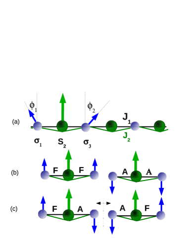
Figure 1: (Color online) (a) Sketch of the mixed-spin chain, Eq. (1), and the three-spin cluster used to construct the classical phase diagram. $\Phi_{1}$ and $\Phi_{2}$ are the variational parameters fixing the directions of the $\sigma$ spins. (b,c) Four cluster ground-state configurations used as building blocks for construction of the classical phases. The doubly degenerate cluster state (c) suggests a $2^{L}$-fold degeneracy of the classical D phase. F an A stand, respectively, for FM and AFM orientations of both classical spins on a bond.

The established cluster states may be used as building blocks to construct optimal $L$-cell spin configurations, by fitting the directions of the sharing $\sigma$ spins of neighboring blocks. By construction, such states correspond to local minima of the classical energy. Clearly, there are unique global spin configurations constructed only from $FF$ or $AA$ three-spin blocks representing, respectively, the classical FM and (Néel-type) FiM phases. On the other hand, to construct the manifold of GS’s realized in the parameter region $\frac{\pi}{4}\leq t\leq\frac{3\pi}{4}$ (sector D on the phase diagram in Fig. 3), we have to find all possible configurations by using the building blocks $FA$ and $AF$ and their counterparts with opposite spin directions. As the number of possible ways to attach a new block to a given global configuration is two, the degeneracy of the classical ground state in this region is exponentially large ($2^{L}$). The established classical phase diagram was additionally confirmed by classical Monte Carlo simulations.

Generally speaking, quantum fluctuations may be expected to reduce the classical degeneracy of the D phase and to favor some subset of classical states. A peculiarity of the three-site interaction in Eq. (1) is that even at a classical level it promotes only collinear spin configurations. As zero-point fluctuations as a rule exhibit the same tendency, it may be speculated that in the quantum case the stabilized phases will inherit this peculiarity of the classical model. In fact, the following analysis of the quantum model confirms the above suggestion. Another special property of the classical three-site interaction is the obvious tendency (for $J_{2}>0$) towards local symmetry breaking of the nearest-neighbor spin correlations. This leads in the quantum system (see below) to a specific clustering and the formation of local nearest-neighbor composite-spin states. Finally, the systems with integer and half-integer cell spins $S+\sigma$ may be expected to exhibit different quantum phases in the $D$ sector. Indeed, according to the generalized Lieb-Schultz-Mattis theorem affleck1 (applicable to systems with half-integer cell spins $S+\sigma$), such systems can have either non-degenerate gapless GS’s or gapped degenerate GS’s with a broken lattice symmetry.

3 Some exact results

3.1 One-magnon states of the FM phase

In the alternating-spin $(S,\sigma)$ chain, there are two types of one-spin-flip excitations above the fully polarized FM state $|F\rangle=|\sigma_{1}S_{2}\sigma_{3}S_{4}\ldots\sigma_{2L-1}S_{2L}\rangle$, which can be written as $|2m\rangle=S_{2m}^{-}|F\rangle$ and $|2m-1\rangle=\sigma_{2m-1}^{-}|F\rangle$, where $S_{2m}^{-}=S_{2m}^{x}-\imath S_{2m}^{y}$ and $\sigma_{2m-1}^{-}=\sigma_{2m-1}^{x}-\imath\sigma_{2m-1}^{y}$ ($m=1,2,\ldots,L$). A simple inspection of the action of the Hamiltonian $\cal{H}_{\sigma S}$ on these states gives the following exact dispersion relations for the one-magnon excited states above the FM state

$$E^{(\pm)}_{k}=a_{k}\pm\sqrt{b_{k}^{2}+c_{k}^{2}},$$ (2)

where $a_{k}=-(S+\sigma)\,\kappa-2\sigma S\sin t\,\sin^{2}(ka_{0})$, $b_{k}=(S-\sigma)\,\kappa+2\sigma S\sin t\,\sin^{2}(ka_{0})$, $c_{k}=2\sqrt{S\sigma}\,\kappa\,\cos(ka_{0})$, $\kappa=\cos t+\sigma\left(2S-1\right)\sin t$, and $a_{0}$ is the lattice spacing.

As may be expected, there are two different types of one-magnon excitations belonging to the gapless $E_{k}^{(-)}$ and optical $E_{k}^{(+)}$ branches. It is easy to check that the expressions for the instability points $t_{F}$ and $t_{F}^{{}^{\prime}}$ ($t_{F}<t^{{}^{\prime}}_{F}$) of the one-magnon excitations, entirely determined by the gapless branch $E_{k}^{(-)}$, read

$$\cos t_{F}+2\sigma S\left(1+\frac{1}{2S}\right)\sin t_{F}=0$$

$$\cos t_{F}^{{}^{\prime}}+2\sigma S\left(1-\frac{1}{2S}\right)\sin t_{F}^{{}^{\prime}}=0.$$

In the case $(S,\sigma)=(1,\frac{1}{2})$, $t_{F}=\pi-\arctan\left(\frac{2}{3}\right)$ and $t_{F}^{{}^{\prime}}=2\pi-\arctan(2)$. At both instability points, $E_{k}^{(-)}$ softens in the whole Brillouin zone, whereas $E_{k}^{(+)}$ keeps its gap structure at $t=t_{F}$, but reduces to the gapless form $E_{k}^{+}=-4\sigma S\sin t_{F}^{{}^{\prime}}\sin^{2}(ka_{0})$ at $t_{F}^{{}^{\prime}}$. As proved below, the instability point $t_{F}$ coincides with one of the exact quantum boundaries of the FM phase in Fig. 3, whereas $t_{F}^{{}^{\prime}}$ is not related to the phase boundaries.

3.2 Three-spin cluster model

Some valuable information concerning the quantum phase diagram of Eq. (1) can be extracted already from the three-site cluster model defined by one of the local Hamiltonians in Eq. (1), say, $h_{1}$. For $\sigma=\frac{1}{2}$, it is instructive to recast $h_{1}$ in the form

$$h_{1}=J_{1}^{{}^{\prime}}\boldsymbol{S}_{2}\cdot\boldsymbol{\sigma}_{13}+J_{2}\,\left(\boldsymbol{S}_{2}\cdot\boldsymbol{\sigma}_{13}\right)^{2}-\frac{J_{2}}{2}S(S+1),$$ (3)

where $J_{1}^{{}^{\prime}}=J_{1}+J_{2}/2$ and $\boldsymbol{\sigma}_{13}=\boldsymbol{\sigma}_{1}+\boldsymbol{\sigma}_{3}$. The spin operators $\boldsymbol{\sigma}_{13}$ and $\boldsymbol{S}_{T}=\boldsymbol{S}_{2}+\boldsymbol{\sigma}_{13}$ define the good quantum numbers $\sigma_{13}=0,1$ and $S_{T}=S\pm\frac{1}{2}$, which are used to classify the eigenvalues and eigenstates of $h_{1}$ (for $S=1$, see Table 1).

$S_{T}$	$\sigma_{13}$	$\hskip 28.45274pt\varepsilon$	Eigenstates
0	1	$-2\cos t+2\sin t$	$|S\rangle=\frac{1}{\sqrt{3}}(\xi^{+}\eta^{-}\!+\!\xi^{-}\eta^{+}$
			$|S\rangle=$ $-\xi^{0}\eta^{0})$
1	1	$-\cos t-\frac{1}{2}\sin t$	$|T_{1}^{0}\rangle=\frac{1}{\sqrt{2}}(\xi^{+}\eta^{-}\!-\!\xi^{-}\eta^{+})$
1	0	$-\sin t$	$|T_{2}^{0}\rangle=\xi^{0}\eta^{s}$
2	1	$\cos t+\frac{1}{2}\sin t$	$|Q^{0}\rangle=\frac{1}{\sqrt{6}}(\xi^{+}\eta^{-}\!+\!\xi^{-}\eta^{+}$
			$|Q^{0}\rangle=$ $+2\xi^{0}\eta^{0})$

Table 1: The eigenvalues $\varepsilon$ and eigenstates of the cluster Hamiltonian $h_{1}$ for $S=1$ and $\sigma=\frac{1}{2}$ in terms of the good quantum numbers $\sigma_{13}$ and $S_{T}$. $\xi^{\mu}$ and $\eta^{\mu}$ ($\mu=0,\pm 1$) are, respectively, the canonical basis states of $\boldsymbol{S}_{2}$ and the composite operator $\boldsymbol{\sigma}_{13}=\boldsymbol{\sigma}_{1}+\boldsymbol{\sigma}_{3}$ in the triplet $\sigma_{13}=1$ state. $\eta^{s}=\frac{1}{\sqrt{2}}(\uparrow_{1}\downarrow_{3}-\downarrow_{1}\uparrow_{3})$ is the singlet ($\sigma_{13}=0$) eigenstate of $\boldsymbol{\sigma}_{13}$. For brevity, only the $0$ components of the triplet and quintet states are presented.

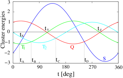
Figure 2: (Color online) Energy levels of the 3-site cluster vs. $t$. $S$, $T_{i}$ ($i=1,2$), and $Q$ are shortcuts of the singlet, triplet, and quintet states in Table 1. $t_{A}=\arctan\left(\frac{2}{5}\right)\approx 21.80^{\circ}$, $t_{X}=\arctan\left(\frac{2}{3}\right)\approx 33.69^{\circ}$, $t_{B}=\arctan\left(2\right)\approx 63.43^{\circ}$, $t_{Y}=\pi-\arctan\left(2\right)\approx 116.57^{\circ}$, $t_{C}=\pi-\arctan\left(\frac{2}{3}\right)\approx 146.31^{\circ}$, $t_{D}=\pi+\arctan(2)\approx 243.43^{\circ}$, and $t_{Z}=2\pi-\arctan\left(2\right)\approx 296.57^{\circ}$. Some special properties of the crossing points are discussed in the text.

In what follows we prove that $t_{F}$ is an exact phase boundary of the FM phase. To this end, let us firstly discuss the structure of the energy levels of $h_{1}$ presented in Table 1 and Fig. 2 for different values of the parameter $t$. There are four regions in the whole parameter space (separated by the crossing points $t_{A}$, $t_{B}$, $t_{C}$, and $t_{D}$), where the cluster system exhibits different GS’s. Denoting by $\varepsilon_{g}=\varepsilon_{g}(t)$ the GS energy of $h_{1}$, the cluster theorem implies that $\varepsilon_{g}$ serves as an exact lower bound for the GS energy per cell $E_{0}/L$ of the quantum Hamiltonian $\cal{H}_{\sigma S}$. Since the energy of the quintet state $|Q^{0}\rangle$ coincides with the energy per site of the FM phase (see Table 1), we conclude that the FM state is the GS of Eq. (1) in the region $t_{C}\leq t\leq t_{D}$, where $|Q^{0}\rangle$ is a cluster GS. Moreover, since the FM phase is gapless, the generalized Lieb-Schultz-Mattis theorem implies that there are no other GS’s. Finally, since $t_{C}$ coincides with the one-magnon instability point $t_{F}$ of the FM phase, we conclude that $t_{F}$ is also an exact quantum phase boundary of the FM phase. Notice that the other boundary $t_{D}$ of the quintet state can not be directly related to the other $FM$ phase boundary $t_{3}$ in Fig. 3 because the one-magnon instability point $t_{F}^{{}^{\prime}}$ lies beyond the region $t_{C}<t<t_{D}$. As a matter of fact, the DMRG estimate $t_{3}\approx 253.08^{\circ}$ implies that $t_{D}<t_{3}<t_{Z}$, whereas the instability point $t_{F}^{{}^{\prime}}$ coincides with the crossing point $t_{Z}$.

The established connection between crossing points in Fig. 2 and some special points on the quantum phase diagram, Fig. 3, can be further extended as follows.
(i) $t_{X}$: At this point, $h_{1}$ is recast to the form $h_{1}=J_{2}\bar{h_{1}}-J_{2}-J_{2}S(S+1)/2$, where $\bar{h_{1}}=\left(1+\boldsymbol{S}_{2}\cdot\boldsymbol{\sigma}_{13}\right)^{2}$ and $J_{2}>0$. Since $\bar{h_{1}}|T_{1}^{\mu}\rangle=0$, the numerical DMRG estimate for the GS matrix element $\langle\bar{h_{1}}\rangle\approx 0.006$ implies that the GS at $t=t_{X}$ is predominantly constructed from local spin configurations related to the triplet cluster states $|T_{1}^{\mu}\rangle$.
(ii) $t_{B}$ ($J_{1}^{{}^{\prime}}=J_{2}>0$): This point appears in the middle of the non-magnetic region in Fig. 3. At $t=t_{B}$, the cluster Hamiltonian $h_{1}$ is proportional to the projector operator ${\cal P}_{1}=1-\frac{1}{2}\boldsymbol{S}_{2}\cdot\boldsymbol{\sigma}_{13}-\frac{1}{2}\left(\boldsymbol{S}_{2}\cdot\boldsymbol{\sigma}_{13}\right)^{2}$ projecting onto the subspace spanned by the triplet states $|T_{1}^{\mu}\rangle$ and $|T_{2}^{\mu}\rangle$. In terms of the projectors ${\cal Q}_{n}=1-{\cal P}_{n}$,

$${\cal H}_{\sigma S}=2J_{2}\sum_{n=1}^{L}{\cal Q}_{n}-J_{2}L,\hskip 5.69046ptJ_{2}>0.$$

This means that at $t=t_{B}$ the GS of ${\cal H}_{\sigma S}$ may be sought as an optimal product state composed of local triplet states ($|T_{1}^{\mu}\rangle$ and $|T_{2}^{\mu}\rangle$).
(iii) $t_{Y}$ ($J_{1}^{{}^{\prime}}=0$, $J_{2}>0$): Relatively close to this point (around $t=t_{2}$) there are pronounced changes of the short-ranged (SR) correlator $\langle\boldsymbol{S}_{2n}\cdot\boldsymbol{S}_{2n+2}\rangle$, indicating a quantum phase transition between the magnetic PP and non-magnetic N phases in Fig. 3.

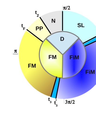
Figure 3: (Color online) Classical (inner circle) and quantum (outer circle) phase diagrams of the (1,$\frac{1}{2}$) model, Eq. (1) vs $t$ ($0\leq t<360^{\circ}$). FM and FiM denote classical ferromagnetic and Néel-type ferrimagnetic phases, respectively, whereas D stands for the classical $2^{L}$-fold degenerate phase. SL, N, and PP stand, respectively, for the the spin-liquid, nematic-like and partially polarized phases. The sectors $t_{1}^{{}^{\prime}}<t<t_{1}$ and $t_{3}<t<t_{3}^{{}^{\prime}}$ are occupied by intermediate partially-polarized phases described in text. $t_{F}=\pi-\arctan\left(\frac{2}{3}\right)$ ($\approx 146.31^{\circ}$) is an exact FM phase boundary. The DMRG estimates for the other phase boundaries read as follows. $t_{1}^{{}^{\prime}}=25.03^{\circ}$, $t_{1}\simeq 30^{\circ}$, $t_{2}\simeq 120^{\circ}$, $t_{3}=253.08^{\circ}$, and $t_{3}^{{}^{\prime}}=264.0^{\circ}$.

4 Quantum phase diagram

Most of the the numerical results in this Section are obtained by DMRG simulations and concern properties of the quantum phase diagram of model (1) in the extreme quantum case $(S,\sigma)=(1,\frac{1}{2})$, Fig. 3 (outer circle). As a rule, there have been performed 7 DMRG sweeps, keeping up to 500 states in the last sweep. The above conditions ensure a good convergence up to 256 unit cells, with a discarded weight of the order of $10^{-8}$ or better.

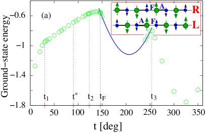
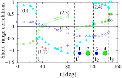
Figure 4: (Color online) (a) DMRG results (OBC, $L=100$) for the GS energy per cell of the $(1,\frac{1}{2})$ chain as function of $t$. The line shows the exact GS energy of the FM state. $t_{1}$, $t^{*}\simeq\frac{\pi}{2}$, $t_{2}$, $t_{F}$, and $t_{3}$ are the phase transition points displayed in Fig. 3. Inset: The cluster configurations $|\Psi_{L}\rangle$ and $|\Psi_{R}\rangle$ selected by the two types of OBC. (b) DMRG results for some SR spin-spin correlators of the $(1,\frac{1}{2})$ chain as a function of $t$. The symbols $(i,j)$ are shortcuts of the isotropic spin-spin correlators between the spins at sites $i$ and $j$ (OBC, $L=100$).

To begin with, let us discuss the general structure and some peculiarities of the quantum phase diagram, Fig. 3, related to the three-body exchange interaction. Some features of the diagram are encoded in the behavior of the SR correlators presented in Fig. 4. As may be expected, the most complex behavior (with abrupt changes of the SR correlators) appears in the region characterized by a manifold of degenerate classical GS configurations (D sector in Fig. 3). As argued below, the abrupt changes of the SR correlator $\langle\boldsymbol{S}_{2n}\cdot\boldsymbol{S}_{2n+2}\rangle$ around the points $t_{F}$ and $t_{2}$ are related with the emergence of partially-polarized states mediating the transition from the FM to a non-magnetic (N) state. In fact, it occurred that the destruction of both classical magnetic phases (FM and FiM) takes place only through intermediate (partially-polarized) states, located in the sectors $(t_{1}^{{}^{\prime}},t_{1})$, $(t_{2},t_{F})$ and $(t_{3},t_{3}^{{}^{\prime}})$ in Fig. 3.

The mentioned clustering effect of the three-body interaction is characteristic for the (non-magnetic) SL sector in Fig. 3 and suggests an establishment of the alternating-bond GS structure $uvuv\ldots$ with $u\neq v$, where $u=\langle\boldsymbol{S}_{2n}\cdot\boldsymbol{\sigma}_{2n-1}\rangle$ and $v=\langle\boldsymbol{S}_{2n}\cdot\boldsymbol{\sigma}_{2n+1}\rangle$ ($n=1,\ldots,L$). Clearly, in the periodic chain there are two equivalent types of ”dimerized” states [denoted by $|\Psi_{L}\rangle$ and $|\Psi_{R}\rangle$ in the Inset of Fig. 4(a)], which correspond to both types of clustering ($uv$ and $vu$) of the local Hamiltonians $h_{n}$ in Eq. (1). The clustering effect is strongly pronounced especially in the middle of the SL region (i.e., close to the point $t_{B}\approx 63.43^{o}$, Fig. 2), where the values $(u,v)\approx(-1,\frac{1}{3})$, red crosses and green squares in Fig. 4 (b), indicate the formation of almost pure spin-$\frac{1}{2}$ states of the composite cell spin $\boldsymbol{S}_{2s}+\boldsymbol{\sigma}_{2n-1}$. $|\Psi_{L}\rangle$ and $|\Psi_{R}\rangle$ are related by the site parity operation ${\cal P}|\Psi_{L,R}\rangle=|\Psi_{R,L}\rangle$. It is important to emphasize that the established clustering does not violate the original translation symmetry by two lattice sites of the Hamiltonian (1). As demonstrated in the Inset of Fig. 4(a), the two types of cluster states can be stabilized by using two different types of open boundary conditions (OBC).

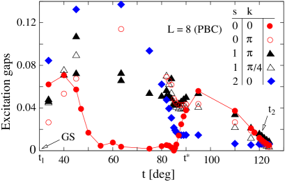
Figure 5: (Color online) Numerical exact diagonalization (ED) results for the low-lying excitation gaps in the periodic $L=8$ $(1,\frac{1}{2})$ system, Eq. (1), as functions of the parameter $t$. Inset: spins ($s$) and wave vectors ($k$) of the excitations. In the region $t_{1}\lesssim t\lesssim t^{*}$, the lowest excited state is a singlet, which scales exponentially with $L$ to the GS. Close to $t=t^{*}\approx\frac{\pi}{2}$ the quintet excitation ($s=2$) is soften and becomes the lowest excitation for $t>t^{*}$.

In finite periodic chains, the symmetry $\cal P$ is not violated, so that we can expect two lowest quasi-degenerate states related to the symmetric (antisymmetric) combinations $|\Psi_{\pm}\rangle=\frac{1}{\sqrt{2}}\left(|\Psi_{L}\rangle\pm|\Psi_{R}\rangle\right)$. As seen in Fig. 5, the expected structure of the spectrum with a singlet lowest-lying excitation is revealed even in small rings. In fact, the performed finite-scaling scaling (FSS) analysis – using additional DMRG results for larger periodic systems – implies that in the SL region the lowest singlet excitation scales exponentially fast with $L$ to the singlet GS, the characteristic length being strongly dependent on the parameter $t$. As discussed below, such a doubling of the spectrum can be identified as well for triplet lowest-lying states. Finally, the numerical ED results presented in Fig. 5 imply a different structure of the states in the non-magnetic region $t^{*}<t<t_{2}$ which is characterized by a quintet ($s=2$) lowest-lying excited state.

4.1 Intermediate magnetic states

In this Subsection, we discuss properties of the intermediate partially-polarized magnetic states identified close to the boundaries of the classical FM and FiM phases in the sectors PP, $t_{1}^{{}^{\prime}}<t<t_{1}$, and $t_{3}<t<t_{3}^{{}^{\prime}}$ (see Fig. 3). These states do not appear in the classical phase diagram.

(i) Magnetic states in the the sector $t_{1}^{{}^{\prime}}<t<t_{1}$:

Denoting by $E(M)$ the lowest-energy eigenvalue in the subspace defined by the z component of the total spin $M$, the gap of the one-magnon AFM branch of excitations in the FiM phase reads $\Delta_{A}=E(M+1)-E(M)$. Here $M=(S-\sigma)L=L/2$ defines the GS sector of the Lieb-Mattis-type FiM phase characterized by the cell magnetic moment $m_{0}\equiv M/L=\frac{1}{2}$. A major effect of the competing three-body interaction in Eq. (1) is the monotonic reduction of the gap with $t$ in the whole $t>0$ region, up to the point $t_{1}^{{}^{\prime}}=25.03^{\circ}$ where $\Delta_{A}$ vanishes, Fig. 6. In the same interval, the local magnetic moments $m_{S}=\langle S_{2n}^{z}\rangle$ and $m_{\sigma}=\langle\sigma_{2n-1}^{z}\rangle$ exhibit non-monotonic behavior. In particular, they reach their extremal values (maximum and minimum, respectively) around one of the crossing points of the cluster model, namely, $t_{A}=\arctan(\frac{2}{5})\approx 21.8^{\circ}$ AKLT . The magnetic moments remain finite at the critical point $t_{1}^{{}^{\prime}}$ ($m_{S}=0.78$ and $m_{\sigma}=0.28$). As may be expected, the quantized magnetization $m_{0}=\frac{1}{2}$ – а characteristic property of the Lieb-Mattis type phases – remains unchanged in the whole FiM region in Fig. 3, up to the transition point $t_{1}^{{}^{\prime}}$.

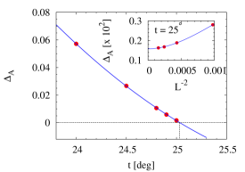
Figure 6: (Color online) DMRG results (red filled circles: $L=64$, PBC) for the AFM gap $\Delta_{A}$ vs $t$ of the FiM phase close to the point $t_{1}^{{}^{\prime}}$ where $\Delta_{A}(t_{1}^{{}^{\prime}})=0$. The solid line represents the fit to the data obtained by the three-parameter ansatz $\Delta_{A}(t)=b_{0}+b_{1}t+b_{2}t^{2}$. The Inset shows the FSS data for $\Delta_{A}(L)$ at $t=25^{\circ}$ (red filled circles) and the fit (solid line) obtained by the ansatz $\Delta_{A}(L)=\Delta_{A}(\infty)+a_{1}/L^{4}+a_{2}/L^{6}$ (solid line), where $\Delta_{A}(\infty)=0.00158$.

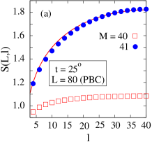
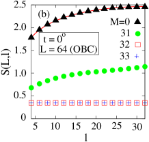
Figure 7: (Color online) DMRG results for the entanglement entropy of different states of the $(1,\frac{1}{2})$ system [(a) $t=25^{\circ}$ and (b) $t=0^{\circ}$] as function of the number of subblock cells $l$. The solid lines represent the analytical result, Eq. (4), for $(\eta,c)=(1,1)$ and $(\eta,c)=(2,2.5)$ in the first and second plots, respectively. The lowest-energy ($M=\frac{L}{2}$) state corresponds to the GS of a Lieb-Mattis-type FiM phase. The lowest-energy ($M=\frac{L}{2}+1$) excited states, corresponding to one-magnon AFM excitations, show different entropy behaviors, approximately corresponding to central charges $c=0$ and $1$ of the system at $t=0^{\circ}$ and $25^{\circ}$, respectively.

The effect of the three-body interaction is reminiscent of the effect of an applied magnetic field in Heisenberg ferrimagnets. A strong magnetic field closes the gap $\Delta_{A}$ and drives the system into a Luttinger-liquid-type magnetic state, which is characterized by a critical AFM mode and a gapped low-lying FM branch of excitations. However, since the three-body interaction does not violate spin rotation symmetries of the Hamiltonian, both interactions might produce different states. An interesting example is the spontaneously magnetized Luttinger-liquid state with gapless AFM and FM branches of excitations predicted for a number of frustrated 1D ferrimagnetic systems smtll .

In Fig. 7, we present DMRG results for the entanglement entropies $S(L,l)$ of different low-lying states at $t=0^{\circ}$ and $25^{\circ}$. The well-known analytical result for the GS entanglement entropy in critical conformally-invariant 1D systems reads holzhey

$$S(L,l)=\frac{c}{3\eta}\ln\left[\frac{\eta L}{\pi}\sin\left(\frac{\pi l}{L}\right)\right]+\mathrm{const}.$$ (4)

Here $l$ is the number of unit cells in the subblock ($l=1,\ldots,L$), $c$ is the central charge, and $\eta=1,2$ for PBC and OBC, respectively. A remarkable fact is that the above analytical expression is also applicable in the case of some pure excited states that correspond to primary fields in conformal field theory alcaraz . Figure 7(a) demonstrates that the entanglement entropy of the lowest-energy state in the $M+1$ sector closely follows the analytical expression for $c=1$. Thus, it can be suggested that at the critical point $t_{1}^{{}^{\prime}}$ the system is spontaneously driven into a gapless Luttinger-liquid-type magnetic state. For comparison, the same excited state in the unfrustrated model ($J_{2}=0$) exhibits a constant entropy corresponding to the central charge $c=0$, Fig. 7(b). Note also the curious observation that the entanglement entropy of the lowest-energy $M=0$ state of the unfrustrated ferrimagnet perfectly reproduces the analytical result in Eq. (4) for $c=\frac{5}{2}$.

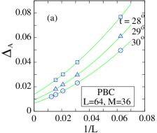
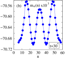
Figure 8: (Color online) (a) DMRG results for the finite-size scaling of the AFM gaps $\Delta_{A}=E(M+1)-E(M)$ in the plateaux state with magnetization $m_{0}=\frac{9}{16}$. The solid lines represent the optimized least-squares fitting functions $\Delta_{A}=c_{0}+c_{1}/L+c_{2}/L^{2}$. The extrapolated gap for $t=30^{\circ}$ is $\Delta_{A}=0.0066$; (b) The local magnetic moment $m_{\sigma}(n)=\langle\sigma_{2n-1}^{z}\rangle$ vs the cell index $n$ in the plateaux phase $m_{0}=\frac{9}{16}$ ($t=30^{\circ}$, $L=64$, PBC). The extremal values of $m_{\sigma}(n)$ correspond to the period $q=16$.

A detailed description of the magnetic phase(s) in the whole interval $t_{1}^{{}^{\prime}}<t<t_{1}$ requires more extensive calculations. For instance, to obtain the GS magnetic moment $M$ – defined as the largest $M$ number with the property $E(M)=E(0)$ – we need a series of lowest-energy eigenvalues $E(M)$ with increasing $M$. In fact, such DMRG calculations were performed for a few points in the above interval, including the boundary point $t=30^{\circ}$ which is supposed to lie close to the phase transition point. The numerical results (up to $L=64$, PBC) imply a very slight monotonic increase of the GS magnetization $m_{0}$ from $\frac{1}{2}$ ($t=t_{1}^{{}^{\prime}}$) approximately up to the value $\frac{9}{16}$ at $t=30^{\circ}$. The increase of $m_{0}$ results from a reduction of the (averaged over cells) magnetic moment $\langle m_{S}(n)\rangle$ from $0.79$ ($t=25^{\circ}$) down to $0.63$ ($t=30^{\circ}$). In the same interval, the magnetic moment $\langle m_{\sigma}(n)\rangle$ increases from $-0.29$ up to the value $-0.07$. The abrupt change of the correlations $\langle\boldsymbol{S}_{2n}\cdot\boldsymbol{S}_{2n+2}\rangle$ in the vicinity of $t=30^{\circ}$, Fig. 4(b), suggests a sharp transition to the non-magnetic state. According to the general rule oshikawa

$$q\left(S+\sigma-m_{0}\right)=\mathrm{integer},$$ (5)

the magnetization $m_{0}=\frac{9}{16}$ may be related to a gapped plateau phase characterized by a periodic magnetic structure with a period $q=16$ unit cells. As a matter of fact, the numerical results for $m_{\sigma}(n)$, Fig. 8(b), reveal such a periodic structure, albeit with extremely small amplitudes of magnetic oscillations. DMRG estimates for the AFM gap $\Delta_{A}$ of the $m_{0}=\frac{9}{16}$ state, Fig. 8(a), imply a smooth reduction of $\Delta_{A}$ with $t$ from $0.0160$ ($t=28^{\circ}$) down to the value $0.0066$ ($t=30^{\circ}$). Unfortunately, due to strong boundary effects – resulting from the extreme smallness of the local magnetic moments $m_{\sigma}(n)$ – the suggested plateau state can not be definitely established by larger-scale DMRG calculations under OBC. Thus, it may be speculated that the spontaneously magnetized Luttinger-liquid state established at $t=25.03^{\circ}$ survives up to the transition point about $t\approx 30^{\circ}$, although the numerical results can not definitely exclude the scenario with some intermediate plateaux states in the region $t_{1}^{{}^{\prime}}<t<t_{1}$.

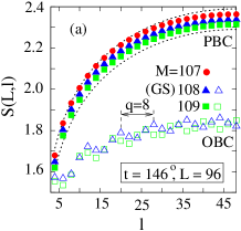
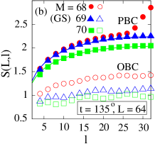
Figure 9: (Color online) DMRG results [filled (PBC) and open (OBC) symbols] for the entanglement entropies $S(L,l)$ vs $l$ of some low-lying states of the $(1,\frac{1}{2})$ model at (a) $t=146^{\circ}$ and (b) $t=135^{\circ}$. Lines: the theoretical result for $S(L,l)$, Eq. (4), with central charge $c=1$. DMRG results imply the GS magnetizations $m_{0}=\frac{9}{8}=1.125$ and $\frac{69}{64}\approx 1.078$ at $t=146^{\circ}$ and $135^{\circ}$, respectively. Under OBC, the function $S(L,l)$ exhibits periodic structures ($q=8$ and $10$) at $t=146^{\circ}$ and $135^{\circ}$, respectively.

(ii) Magnetic states in the PP sector:
As argued above, the exact phase boundary $t_{F}$ coincides with one of the instability points of the one-magnon AFM excitations and is characterized by a complete softening of the dispersion function $E_{k}^{(-)}$, Eq. (2), in the whole Brillouin zone. The transition at $t_{F}$ is signaled by sharp reconstructions of the SR correlations, the jump (with a change of sign) of the correlator $\langle\boldsymbol{\sigma}_{2n-1}\cdot\boldsymbol{\sigma}_{2n+1}\rangle$ being the most important. On the contrary, the nearest-neighbor correlator $\langle\boldsymbol{S}_{2n}\cdot\boldsymbol{S}_{2n+2}\rangle$ remains positive and signals a FM ordering of the spin-$S$ subsystem in the entire PP sector in Fig. 3. Close to the other boundary $t_{2}$ ($\simeq\frac{2\pi}{3}$), the behavior of the nearest-neighbor spin correlations is reversed, namely, the transition to a non-magnetic state is accompanied by an abrupt change of sign of the correlator $\langle\boldsymbol{S}_{2n}\cdot\boldsymbol{S}_{2n+2}\rangle$, whereas the nearest-neighbor $\sigma$-spin correlations remain almost untouched. In fact, the numerical DMRG analysis implies finite sublattice magnetizations [$m_{S}(n),m_{\sigma}(n)>0$] all over the region $t_{2}<t<t_{F}$. Moreover, while the average of $m_{\sigma}(n)$ monotonically decreases from $0.221$ at $t=146^{\circ}$ down to $\approx 0.06$ at $t=123^{\circ}$, the average of $m_{S}(n)$ increases from $0.903$ (at $t=146^{\circ}$) almost to its saturation value $1$ in a vicinity of $t_{2}$, where the correlations between $S$ and $\sigma$ sublattice spins become extremely weak (see Fig. 4) and then sharply drop to zero.

We show in Fig. 9 DMRG results for the entanglement entropies of a few low-lying states at two points ($t=146^{\circ}$ and $135^{\circ}$) corresponding to the GS magnetizations $m_{0}=\frac{9}{8}$ and $m_{0}\approx 1.07$, respectively. The GS entropies at both points approximately follow the theoretical curves corresponding to the central charge $c=1$. The same is true for the lowest-energy states in the neighbor sectors $M\pm 1$ ($M=108$) at $t=146^{\circ}$, whereas at $t=135^{\circ}$ the lowest-energy states in the neighbor $M$ sectors apparently deviate from the theoretical $c=1$ curve. Since an analysis based alone on the entanglement entropy can not definitely exclude the scenario with extremely small gaps, we have performed a separate DMRG test of the AFM gaps $\Delta_{A}$ at both points. The numerical data for $\Delta_{A}(L)$ at fixed GS magnetizations $m_{0}$, Fig. 10, implies extremely small (but finite) extrapolated gaps at both points: $\Delta_{A}=1.7$ x $10^{-4}$ ($6.9$ x $10^{-4}$) at $t=146^{\circ}$ ($135^{\circ}$). These observations resemble the established picture of magnetic states close to the transition point $t_{1}$. As before, it may be suggested that close to $t_{F}$ a plateau $m_{0}=\frac{9}{8}$ state with the period $q=8$ is established. Unlike the state around $t_{1}$, the plateau GS with $m_{0}=\frac{9}{8}$ around $t_{F}$ is additionally supported by larger-scale DMRG results under OBC (up to $L=512$). Notice that the observed critical behavior of some excited states in Fig. 9(a) close to the transition point $t_{F}$ is compatible with the established complete softening of the dispersion function $E_{k}^{(-)}$ at $t=t_{F}$.

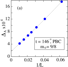
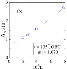
Figure 10: (Color online) Finite-size scaling of the lowest excitation gaps in the states with GS magnetizations (a) $m_{0}=\frac{9}{8}$ ($t=146^{\circ}$) and (b) $m_{0}=1.070$ ($t=135^{\circ}$). The respective $L=\infty$ gaps $\Delta_{A}=1.7$ x $10^{-4}$ and $6.9$ x $10^{-4}$ are extracted from the fitting ansatz $\Delta_{A}(L)=\Delta_{A}+a_{1}/L+a_{2}/L^{2}$ (dot lines).

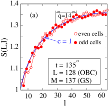
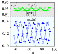
Figure 11: (Color online) (a) DMRG results for the GS entanglement entropies vs $l$ for even- (open circles) and odd-cell (filled circles) subblocks $l$ at $t=135^{\circ}$ (OBC), exhibiting oscillation periods $q=14$. The line shows the theoretical result, Eq. (4), with $c=1$. (b) The local magnetic moments [$m_{S}(n)$ and $m_{\sigma}(n)$] of the same system for even- (open circles) and odd-cell (filled circles) indeces $n$ exhibit the same oscillation periods ($q=14$).

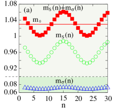
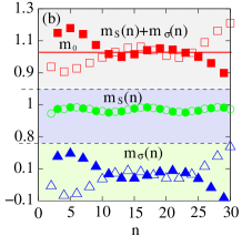
Figure 12: (Color online) DMRG results for the local magnetizations $m_{S}(n)=\langle S_{2n}^{z}\rangle$, $m_{\sigma}(n)=\langle\sigma_{2n+1}^{z}\rangle$ and $m_{0}(n)=m_{S}(n)+m_{\sigma}(n)$ vs cell index $n$ for (a) periodic and (b) open $(1,\frac{1}{2})$ chains ($t=123^{\circ}$, $L=32$, $M=33$). $m_{0}=M/L$ is the GS magnetization. The open/filled symbols in (b) correspond to even/odd $n$. The magnetization profiles in (b) suggest a R-type OBC (i.e., $\sigma$ spin on the right end). Note the different scales of $y$ axes of both plots.

Another intriguing feature of the entanglement entropies under OBC shown in Figs. 9 and 11(a) is their periodic structure. At $t=146^{\circ}$, the period $q=8$ of $S(L,l)$ coincides with the expected period of the plateau state with magnetization $m_{0}=\frac{9}{8}$ [see Eq. (5)]. The common origin of both periods is further supported by the numerical results for the entropy $S(L,l)$ and corresponding magnetization profiles of an open chain at $t=135^{\circ}$, Fig. 11(a). Using these results, it may be speculated that the actual GS at $t=135^{\circ}$ is the plateau $m_{0}=\frac{15}{14}$ state, since the other possible values of $m_{0}$, admitted by Eq. (5), deviate significantly from the DMRG estimate $m_{0}\approx 1.07$. The periodic magnetic patterns in Fig. 11(b), corresponding to even and odd elementary cells, are shifted by a half period. Another obvious effect of the boundaries is the enhancement of the amplitudes of oscillations, especially those related to the magnetic moment $m_{\sigma}(n)$. Actually, the absence of visible periodic structures in the DMRG data for $S(L,l)$ in periodic chains, Fig. 9, is probably due to the extreme smallness of the oscillation amplitudes under PBC.

On approaching the transition point $t_{2}$, the boundary effects in open chains become stronger. A comparison between the established magnetic structures in periodic and open chains at $t=123^{\circ}$ is presented in Fig. 12. An important observation in the case of periodic chains, Fig. 12(a), is the strongly enhanced amplitude of the $m_{S}(n)$ oscillations, which dominates by an order of magnitude the amplitude related to the $\sigma$ spins. Note that the amplitude and the profile of $m_{S}(n)$ remain almost unchanged in both cases, apart from a phase shift and some modifications close to the end spins. On the contrary, as seen in Fig. 12(b), the OBC notably modifies the magnetic structure related with the $\sigma$ spins, the most impressive being the strong enhancement of the local magnetizations $m_{\sigma}(n)$ spreading deep in the bulk.

In conclusion, we find a convincing numerical support for a plateau $m_{0}=\frac{9}{8}$ state close to the FM phase boundary $t=t_{F}$. Due to strong FSS effects, it is difficult to track the development of this magnetic state as $t$ is changed down to $t=t_{2}$, where the phase transition to a non-magnetic state takes place. As in the case of $t_{1}^{{}^{\prime}}<t<t_{1}$, we may speculated that the region is occupied by an incommensurate Luttinger-liquid magnetic state. However, as seen from the DMRG data at $t=135^{\circ}$, the scenario with some intermediate plateau states can not be definitely excluded.

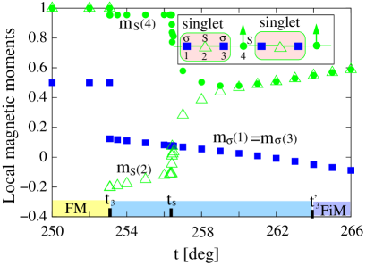
Figure 13: (Color online) DMRG results ($L=32,PBC$) for the local magnetic moments vs $t$ of the doubly degenerate FiM state appearing between the FM and FiM phases. The Inset shows a cartoon of the state in the region $t_{3}<t<t_{s}$. $t_{3}=253.08^{\circ}$, $t_{3}^{{}^{\prime}}=264.0^{\circ}$, and $t_{s}=256.4^{\circ}$.

(iii) Degenerate FiM phase in the sector $t_{3}<T<t_{3}^{{}^{\prime}}$:

Apart from the shift $\frac{3\pi}{2}\rightarrow t_{3}$ of the FM boundary (see Fig. 3), quantum fluctuations also stabilize a new doubly degenerate FiM phase in the vicinity of $t_{3}$ ( $t_{3}<t<t_{3}^{{}^{\prime}}$). Here $t_{3}^{{}^{\prime}}=264.0^{\circ}$ is the new boundary of the FiM phase. In Fig. 13, we show DMRG results for the local magnetic moments $m_{S}(n)$ and $m_{\sigma}(n)$ in two neighboring cells ($n=1,2$). Unlike the standard FiM phase, where the magnetic moment is uniformly distributed between the lattice cells [i.e., $m_{0}(n)=\frac{1}{2}$], the period of the discussed degenerate FiM state includes two lattice cells, where $m_{0}(n)+m_{0}(n+1)=1$, $m_{\sigma}(n)=m_{\sigma}(n+1)$, and $m_{S}(n)\neq m_{S}(n+1)$. The transition to the FM phase at $t_{3}$, a result of level crossing, takes place through abrupt changes of the local magnetic moments. On the contrary, the transition to the FiM phase at $t_{3}^{{}^{\prime}}$ is preceded by a smooth decrease to zero of the order parameter $\delta m=|m_{S}(n+1)-m_{S}(n)|$, $\delta m(t_{3}^{{}^{\prime}})=0$. The gap $\Delta(t)$ between the FiM GS and the excited degenerate state vanishes at the critical point $t_{3}^{{}^{\prime}}$. At $t=t_{3}^{{}^{\prime}}$, the gap scales to zero as $\Delta_{L}(t_{3}^{{}^{\prime}})\propto 1/L$.

The special point $t_{s}$ (where the sign of the correlator $\langle\boldsymbol{S}_{2n}\cdot\boldsymbol{\sigma}_{2n\pm 1}\rangle$ is changed) divides the interval $t_{3}<t<t_{3}^{{}^{\prime}}$ into two regions with different behaviors of the local magnetic moments. Although degenerate, for $t>t_{s}$ the magnetic structure resembles the classical Néel phase. In the Inset of Fig. 13, we show a cartoon of the state in the region $t_{3}<t<t_{s}$ implied by an analysis of the SR correlations close to $t_{s}$. Due to the extreme weakness of the nearest-neighbor correlators $\langle\boldsymbol{S}_{2n}\cdot\boldsymbol{\sigma}_{2n\pm 1}\rangle$ ($n=2,4,\ldots$), one half of the $S$ spins forms an almost saturated magnetic state. On the other hand, the rest of the spins is divided into three-spin clusters, which exhibit SR correlations typical for the cluster singlet state in Table 1.

4.2 The critical spin-liquid phase (SL)

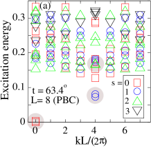
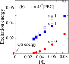
Figure 14: (Color online) (a) Numerical ED results for the low-lying (spin $s=0,1,2$, and $3$) excitation energies of the periodic $L=8$ chain at $t=63.4^{\circ}$. The shaded symbols correspond to the lowest pairs of singlet, triplet and quintet excitations. (b) DMRG results for the finite-size scaling of the lowest singlet and triplet modes at $t=45^{\circ}$.

As noticed above, the $uv$ clustering of the GS in the SL region in Fig. 3 – a special effect of the three-body interaction – presumably results in a double degeneracy of the singlet GS in the large-$L$ limit. As indicated in Fig. 14(a), some low-lying larger-spin states in the ring spectrum also exhibit a tendency towards formation of quasi-degenerate pairs. In fact, even in the region around $t=45^{\circ}$, where the singlet gap in the $L=8$ ring is relatively large, the performed FSS analysis for larger-$L$ rings supports the suggested picture and, in particular, implies an exponentially fast (with $L$) doubling of the lowest singlet and triplet states [see Fig. 14(b)]. Due to strong boundary effects, the discussed doubling in the lowest part of the spectrum remains invisible in open chains up to the largest ($L=256$) simulated system.

Assuming conformal invariance, additional properties of the non-magnetic SL phase can be extracted from the FSS behavior of the GS and the lowest excited states. Since the numerical simulations for periodic chains are hampered by the quasi-degeneracy of the GS, the following analysis is performed under OBC. The expected large-$L$ behavior of the GS energy reads bloete

$$\frac{E_{0}(L)}{L}=e_{\infty}+\frac{f_{s}}{L}-\frac{v_{s}\pi c}{6\gamma L^{2}}+o(L^{-2}),$$ (6)

where $e_{\infty}$ is the bulk GS energy per unit cell, $f_{s}$ is the surface free energy ($f_{s}=0$ under PBC), $v_{s}$ is the spin velocity, $c$ is the central charge, and $\gamma=1,4$ for PBC and OBC, respectively. For OBC, the expected tower of excited states related to some primary operator is defined by cardy

$$\Delta_{n}(L)\equiv E_{n}(L)-E_{0}(L)=\frac{\pi v_{s}}{L}\left(x_{s}+n\right)+o(L^{-1}),$$ (7)

where $n=0,1,2,\ldots$ and $x_{s}$ is the universal surface exponent related to the same operator. The exponent $x_{s}$ is known, in particular, for the energy states of the isotropic spin-$\frac{1}{2}$ Heisenberg chain in the $m$ sectors ($x_{s}^{(m)}=m^{2}$, $m=1,2,\ldots$), where $m$ is the $z$ component of the total spin alcaraz . The Hamiltonian (1) respects the spin-rotation symmetry, so that the above asymptotic expression, when used as a fitting ansatz, have to be supplemented by appropriate logarithmic terms hallberg .

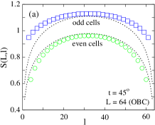
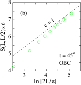
Figure 15: (Color online) (a) Numerical DMRG results for the even- and odd-cells entanglement entropy of the SL state ($t=45^{\circ}$) vs the number of subblock cells $l$. The dot lines represent the theoretical result in Eq. (4) with $c=1$. (b) Extrapolation of the numerical results for the $l=L/2$ entanglement entropy $S(L,L/2)$ vs $\ln(2L/\pi)$ at $t=45^{\circ}$. The dot line corresponds to $S(L,L/2)$ with the central charge $c=1$.

Since the central charge $c$ can be independently obtained from a fit of Eq. (4) to the DMRG data, the asymptotic expression for $E_{0}(L)$ can, in principle, be used to find the non-universal parameters $e_{\infty}$, $f_{s}$ and $v_{s}$. Thus, the surface exponents $x_{s}$ of different primary operators can be extracted by fitting Eq. (7) to the numerical data. However, due to logarithmic corrections, the precise estimate of $v_{s}$ from Eq. (6) for isotropic systems may require numerical simulations of extremely large systems.

In Fig. 15(a), we show DMRG results for the GS entanglement entropy $S(L,l)$ of the open alternating-spin chain at $t=45^{\circ}$ ($L=64$). We observe two different branches of $S(L,l)$ corresponding to even and odd subblock lengths $l$. Similar even-odd oscillations in the entanglement entropy have been firstly reported in open spin-$\frac{1}{2}$ XXZ chains, including the isotropic limit lafforencie . In this work, it was clarified that the alternating part of $S(L,l)$, decaying away from the boundary with a universal power law, appears as a result of oscillations of the energy density. Further, the latter oscillations were related with the tendency of the critical system towards formation of local singlet bonds, combined with the strong tendency of the end spins to form local singlets. As the extrapolation of the numerical data for $S(L,L/2)$ vs $\ln\left(2L/\pi\right)$ up to $L=256$ suggests a critical behavior with central charge $c=1$ [see Fig. 15(b)], to understand the even-odd effect in the alternating spin chain one may suggest a scenario similar. However, the picture looks more complex as the formation of local singlet states in the alternating spin model includes at least four neighboring spins.

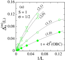
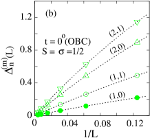
Figure 16: (Color online) (a) Scaling of the lowest triplet [$(m,n)=(1,0)$ and $(1,1)$] and quintet [$(m,n)=(2,0)$ and $(2,1)$] excitation gaps in (a) the alternating spin $S=1$ and $\sigma=\frac{1}{2})$ open chain (DMRG, OBC, $t=45^{\circ}$). (b) Scaling of the related gaps in the uniform spin ($S=\sigma=\frac{1}{2}$) model without three-body terms (DMRG, OBC, $t=0^{\circ}$). The dashed lines show the best fits of $\Delta_{n}^{(m)}(L)=E_{n}^{(m)}(L)-E_{0}(L)$ to the DMRG data (symbols) obtained by Eq. (8.

In Fig. 16, we compare FSS results for the lowest two excitations in the triplet ($m=1$) and quintet ($m=2$) towers of states of the Hamiltonian ${\cal H}_{\sigma S}$, Eq. (1), for two cases: (i) $(S,\sigma)=(1,\frac{1}{2})$ at $t=45^{\circ}$ and (ii) $(S,\sigma)=(\frac{1}{2},\frac{1}{2})$ at $t=0^{\circ}$. The fit of the reduced gaps $L\Delta_{n}^{(m)}$ is performed by the four-parameter ansatz

$$L\Delta_{n}^{(m)}(L)=a_{n}^{(m)}+\frac{b_{n}^{(m)}}{\ln\left(L/\xi_{n}^{(m)}\right)}+\frac{c_{n}^{(m)}}{L}.$$ (8)

For systems belonging to the Gaussian universality class – like the isotropic spin-$\frac{1}{2}$ chain in the second case – the first fitting parameter $a_{n}^{(m)}$ is expected to approach the exact result $a_{n}^{(m)}=\pi v_{s}(m^{2}+n)/2$, which gives $[m,n]\equiv a_{n}^{(m)}/a_{0}^{(1)}=m^{2}+n$. In fact, the performed fits for the $(S,\sigma)=(\frac{1}{2},\frac{1}{2})$ chain give the numerical estimates [1,1]=1.99, [2,0]=3.99, and [2,1]=4.96, which excellently reproduce the expected theoretical ratios. Moreover, a comparison of Eqs. (7) and (8) implies the relation $a_{0}^{(1)}=v_{s}/2$, which gives an estimate for $v_{s}$ deviating only by about $0.6\%$ from the exact result $\pi/2$. For the alternating-spin chain at $t=45^{\circ}$, similar fits give the numerical estimates $v_{s}=0.38$, [1,1]=2.11, [2,0]=4.44, and [2,1]=5.69. In spite of the larger deviations from the theoretical results for $[m,n]$, the observed structure of the lowest-lying part of the spectrum in the alternating-spin model remains close to the structure in the reference spin-$\frac{1}{2}$ Heisenberg chain. As may be expected, in the middle of the range occupied by the SL phase, where the doubling (with L) of the lowest singlet and triplet states is faster (see Fig. 5), the deviations of $[m,n]$ from the expected theoretical results are smaller. For example, at $t=63.4^{\circ}$ the same fitting procedure gives $v_{s}=1.88$, $[1,1]=1.93$, $[2,0]=4.00$, and $[2,1]=5.35$.

The established one-to-one mapping of the lowest-lying excitations of both models suggests similar critical properties. Since the unit cell of the reference spin-$\frac{1}{2}$ model contains two equivalent lattice sites, under PBC this means a doubling of the spectrum and, in particular, two equivalent critical modes. This explains the discussed doubling of the lowest-lying excitations in the alternating-spin $(1,\frac{1}{2})$ ring. Thus, both the GS entanglement entropy as well as the FSS properties of the SL phase point towards a Gaussian type critical behavior. What is changed in the region occupied by the SL phase is the non-universal parameter $v_{s}$. Since the alternating-spin $(1,\frac{1}{2})$ ring exhibits two equivalent critical modes, the SL state may be interpreted as a critical spin-liquid phase described by two Gaussian conformal theories associated with these modes. Similar critical phases have been studied in some exactly solvable models, including spin models with extra three-body exchange interactions. In particular, there is an exactly solvable alternating-spin $(S,\sigma)$ model aladim closely related to the generic model discussed in this work at the point $t=45^{\circ}$. In fact, the difference between both models is reduced to an additional FM exchange term ($h_{n}^{\sigma\sigma}=J_{3}\boldsymbol{\sigma}_{2n-1}\cdot\boldsymbol{\sigma}_{2n+1}$, $J_{3}<0$) in the exactly solvable model. Assuming that $h_{n}^{\sigma\sigma}$ represents an irrelevant operator (in a renormalization group sense), it may be speculated that both models exhibit similar critical properties. In particular, for the exactly solvable $(S,\sigma)$ model, it has been predicted aladim that the critical behavior can be described by an effective central charge which is the sum of the central charges related with two critical modes, t.e., $c_{eff}=3\sigma/(\sigma+1)+3(S-\sigma)/(S-\sigma+1)$. In the special case $(S,\sigma)=(1,\frac{1}{2})$ this gives $c_{eff}=1+1=2$, which coincides with the expected critical behavior of the SL phase.

4.3 Critical nematic-like phase (N)

The behavior of both the low-lying excitations and SR correlations indicate the existence of a different non-magnetic phase in the parameter region $\frac{\pi}{2}\simeq t\simeq\frac{2\pi}{3}$ (N sector in Fig. 3). Indeed, as seen in Fig. 5, in the vicinity of $t\simeq\frac{\pi}{2}$ the quintet ($s=2$, $k=0$) excitation is strongly softened and becomes the lowest excited state up to $t\simeq\frac{2\pi}{3}$. Moreover, the DMRG calculations for somewhat larger periodic systems (up to $L=28$) reveal the same structure of the low-lying part of the spectrum. Unfortunately, slow convergence of the DMRG method in this region hampers more extensive numerical simulations of the FSS properties of the excitation gaps. The picture of SR correlations in this region, Fig. 4, allows to speculate that the properties of the non-magnetic state are mainly controlled by the $S$ subsystem. Indeed, as already discussed above, the correlator $\langle\boldsymbol{S}_{2n}\cdot\boldsymbol{S}_{2n+2}\rangle$ exhibits a strong modification in a vicinity of the second phase boundary ($t=t_{2}$). Meanwhile, the behavior of the SR correlator $\langle\boldsymbol{\sigma}_{2n-1}\cdot\boldsymbol{\sigma}_{2n+1}\rangle$ remains practically unchanged in the entire N sector, including the regions around both phase boundaries. Interestingly, in the entire N sector the typical values of the latter correlator remain relatively close to the value $\frac{1}{4}-\ln(2)\approx-0.443$ characteristic for the isotropic spin-$\frac{1}{2}$ chain. Another peculiarity in this region is the extremely week correlation between the nearest-neighbor $S$ and $\sigma$ spins [see Fig. 4(b)].

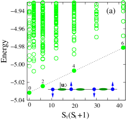
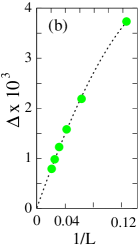
Figure 17: (Color online) (a) Numerical ED results for the energy spectrum of the $(1,\frac{1}{2})$ model, Eq. (1), at $t=110^{\circ}$ as a function of $S_{t}(S_{t}+1)$ ($L=8$, PBC). The numbers denote the spins ($S_{t}$) of the lowest-lying multiplets (filled circles) in the even $S_{t}$ sectors. The dashed line is a guide for the eye. Inset: Cartoon of the suggested nematic-like state in the N sector. The ellipses denote local nematic states on the even $S$ sites. (b) Finite-size scaling of the lowest $S_{t}=2$ gap. The dashed line denotes the least-squares fit to the DMRG data ($t=110^{\circ}$, OBC) obtained by the fitting ansatz $L\Delta(L)=a_{0}+a_{1}/L+a_{2}/L^{2}$.

Further information about the non-magnetic (N) state can be extracted form Fig. 17 showing ED results for the excitation spectrum of the same system at $t=110^{\circ}$ in different total-spin ($S_{t}$) sectors. An obvious feature of the presented spectrum is the established tower of well-separated lowest multiplets containing only even $S_{t}$ sectors. Furthermore, the energies in the tower scale as $E(S)\propto S_{t}(S_{t}+1)$. The observed structure is known as a fingerprint of the spin quadrupolar (i.e., nematic) order lauchli2 , unlike the Anderson tower – a characteristic of the Néel order – containing all $S_{t}$ sectors anderson . In fact, Anderson towers of states have been observed even in some finite isotropic spin-$S$ chains and magnetic molecules schnack , including spin-$\frac{1}{2}$ Heisenberg rings which support a quasi-long-range Néel-type order in the thermodynamic limit eggert . In the same spirit, we consider the specific structure in Fig. 17(a) as a fingerprint of a non-magnetic state with dominant quadrupolar spin fluctuations. The FSS of the quintet excitation gap $\Delta(L)\propto 1/L$, Fig. 17(b), pointing towards a gapless N state, is consistent with the above suggestion.

The Inset of Fig. 17(a) shows the cartoon of a tentative nematic-like state respecting the established properties of the low-lying spectrum and the peculiarities of the SR correlations. In the vector basis $|\alpha\rangle$ ($\alpha=x,y,z$) of the spin-1 operators $\boldsymbol{S}_{2n}$, an arbitrary on-site quadrupolar state can be written in the form $|\boldsymbol{u}_{2n}\rangle=\sum_{\alpha}u_{2n}^{\alpha}|\alpha\rangle$, where $\boldsymbol{u}_{2n}$ is a real unit vector. Since $\langle\boldsymbol{u}_{2n}|S_{2n}^{\alpha}|\boldsymbol{u}_{2n}\rangle=0$ for every $\alpha$, the $|\boldsymbol{u}_{2n}\rangle$ states on the even sites vanish the nearest-neighbor $\sigma S$ correlations for an arbitrary configuration of the $\sigma$ spins, in accord with the established extremely weak nearest-neighbor $\sigma S$ correlations. To reveal the origin of the observed strong AFM nearest-neighbor $\sigma\sigma$ correlations, it is instructive to recast the local three-body exchange term in Eq. (1), which dominates the interactions in the N region, to the following symmetric form

$$h_{n}^{(3)}=J_{2}\boldsymbol{\sigma}_{2n-1}\cdot\hat{\boldsymbol{Q}}_{2n}\cdot\boldsymbol{\sigma}_{2n+1},\,J_{2}>0,$$ (9)

where the symmetric tensor $Q_{2n}^{\alpha\beta}=S_{2n}^{\alpha}S_{2n}^{\beta}+S_{2n}^{\beta}S_{2n}^{\alpha}$ is closely related to the on-site quadrupolar order-parameter operator for the $\boldsymbol{S}_{2n}$ spins (see, e.g., Ref. frustration ). Using the relation $\langle\boldsymbol{u}_{2n}|Q_{2n}^{\alpha\beta}|\boldsymbol{u}_{2n}\rangle=\delta^{\alpha\beta}-u_{2n}^{\alpha}u_{2n}^{\beta}$, the effective zeroth-order Hamiltonian for the $\sigma$ subsystem reads $\bar{h}_{n}^{(3)}\equiv\langle\boldsymbol{u}_{2n}|h_{n}^{(3)}|\boldsymbol{u}_{2n}\rangle=J_{2}\boldsymbol{\sigma}_{2n-1}^{\perp}\cdot\boldsymbol{\sigma}_{2n+1}^{\perp}$, where $\boldsymbol{\sigma}_{2n-1}^{\perp}$ and $\boldsymbol{\sigma}_{2n+1}^{\perp}$ are the transfer components of the $\sigma$ spins in respect to the local vector $\boldsymbol{u}_{2n}$. $\bar{h}_{n}^{(3)}$ defines a kind of AFM spin-$\frac{1}{2}$ XX model with the local quantization axis $\boldsymbol{u}_{2n}$.

In conclusion, both the SR correlations as well as specific structure of the low-lying excitations point towards the establishment of an intriguing critical nematic-like phase in the N region of the phase diagram, Fig. 3, which is characterized by quadrupolar $S$-spin fluctuations. The three-body interaction plays a dominant role, whereas the role of the FM bilinear terms ($J_{1}<0$) is to reduce the AFM correlations between the $S$ and $\sigma$ subsystems. Further properties of this phase as well as more precise estimates for the phase boundaries require other methods (e.g., larger-scale numerical ED simulations), which are beyond the scope of the present work.

5 Summary

We have established the general structure of the quantum phase diagram of a generic 1D isotropic spin model with competing biquadratic three-body exchange interactions, with an emphasis on the minimal model with alternating $S=1$ and $\sigma=\frac{1}{2}$ spins. A number of observed effects as well as specific phases (like the doubly degenerate FiM state, the two-critical-modes spin-liquid, as well as the nematic-like phase) can be attributed to peculiarities of the three-body exchange interaction, such as the promotion of collinear spin configurations and pronounced tendency towards a nearest-neighbor clustering of the spins. It may be expected that most of the predicted effects and phases persist (or are stabilized) in higher space dimensions. On the experimental side, we believe that the presented results will encourage the search for real systems exhibiting three-body exchange interactions. In this respect, the alternating-spin materials with complex unit cells constitute a promising background of systems principally allowing manipulations of the higher-order exchange interactions.

References

- (1) Introduction to Frustrated Magnetism: Materials, Experiments, Theory, edited by C. Lacroix, P. Mendels, and F. Mila, Springer Series in Solid-State Sciences, Vol. 164 (2011).
- (2) see, e.g., A. Läuchli, G. Schmid, and S. Trebst, Phys. Rev. B 74, 144426 (2006), and references therein
- (3) K. Harada and N. Kawashima, Phys. Rev. B 65, 052403 (2002)
- (4) T. A. Tóth, A. M. Läuchli, F. Mila, and Karlo Penc, Phys. Rev. B 85, 140403(R) (2012)
- (5) T. Momoi, P. Sindzingre, and N. Shannon, Phys. Rev. Lett. 97, 257204 (2006)
- (6) A. Smerald and N. Shannon, Phys. Rev. B 88, 184430 (2013)
- (7) U. Falk, A. Furrer, H. U. Güdel, and J. K. Kjems, Phys. Rev. Lett. 56, 1956 (1986)
- (8) U. Falk, A. Furrer, J. K. Kjems, and H. U. Güdel, Phys. Rev. Lett. 52, 1336 (1984)
- (9) T. Iwashita and N. Uryû, J. Phys. Soc. Jpn. 36, 48 (1974)
- (10) A. Furrer, Int. J. Mod. Phys. B 24, 3653 (2010); A. Furrer and O. Waldmann, Rev. Mod. Phys. 85, 367 (2013)
- (11) F. Michaud, F. Vernay, S. R. Manmana, and F. Mila, Phys. Rev. Lett. 108, 127202 (2012)
- (12) J. K. Pachos and M. B. Plenio, Phys. Rev. Lett. 93, 056402 (2004)
- (13) H. P. Büchler, A. Micheli, and P. Zoller, Nature Physics 3, 726 (2007)
- (14) N. Andrei and H. Johannesson, Phys. Lett. A 100, 108 (1984)
- (15) H. J. de Vega and F. Woynarovich, J. Phys. A: Math. Gen. 25, 4499 (1992)
- (16) S. R. Aladim and M. J. Martins, J. Phys. A: Math. Gen. 26, L529 (1993)
- (17) H. J. de Vega, L. Mezincescu, and R. I. Nepomechie, Phys. Rev. B 49, 13223 (1994)
- (18) A. Bytsko and A. Doikou, J. Phys. A: Math. Gen. 37, 4465 (2004)
- (19) G. A. P. Ribeiro and A. Klümper, Nucl. Phys. B 801 [FS], 247 (2008)
- (20) F. Michaud, S. R. Manmana, and F. Mila, Phys. Rev. B 87, 140404(R) (2013)
- (21) F. Michaud, and F. Mila, Phys. Rev. B 88, 094435 (2013)
- (22) Z.-Y. Wang, S. C. Furuya, M. Nakamura, and R. Komakura, Phys. Rev. B 88, 224419 (2013)
- (23) Ch. P. Landee and M. M. Turnbull, Eur. J. Inorg. Chem. 2013, 2266 (2013)
- (24) N. B. Ivanov, J. Richter, and J. Schulenburg, Phys. Rev. B 79, 104412 (2009); N. B. Ivanov, Condensed Matter Physics 12, 435 (2009)
- (25) I. Affleck and E. H. Lieb, J. Math. Phys. 12, 57 (1986)
- (26) According Eq. (3), formally corresponds to the AKLT point in the BBQ model
- (27) Such a non-Lieb-Mattis-type critical ferrimagnetic state has been originally observed in the phase diagram of the frustrated mixed-spin two-leg ladder system [N. B. Ivanov and J. Richter, Phys. Rev. B 69, 214420 (2004)]. For other spin systems exhibiting this state see, e.g., T. Shimokawa and H. Nakano, J. Kor. Phys. Sos. (SI) 63, 591 (2013) and references therein. The theory of this state has recently been developed in: Sh. S. Furuya and Th. Giamarchi, Phys. Rev. B 89, 205131 (2014).
- (28) C. Holzhey, F. Larsen, and F. Wilczek, Nucl. Phys. B 424, 443 (1994); P. Calabrese and J. Cardy, J. Stat. Mech. 06, P06002 (2004).
- (29) F. C. Alcaraz, m. I. Berganza, and G. Sierra, Phys. Rev. Lett. 106, 201601 (2011)
- (30) M. Oshikawa, M. Yamanaka, and I. Affleck, Phys. Rev. Lett. 78, 1984 (1997)
- (31) H. W. J. Blöte, J. L. Cardy, and M. P. Nightingale, Phys. Rev. Lett. 56, 742 (1986); I. Affleck, ibid. 56, 746 (1986)
- (32) J. Cardy, J. Math. Phys. A: Math. Gen. 17, L385 (1984)
- (33) F. C. Alcaraz, M. N. Barber, M. T. Batchelor, R. J. Baxter, and G. R. W. Quispel, J. Math. Phys. A: Math. Gen. 20, 6397 (1987)
- (34) see, e.g., K. Hallberg, X. Q. G. Wang, P. Horsch, and A. Moreo, Phys. Rev. Lett. 76, 4955 (1996), and references therein
- (35) N. Laflorencie, E. S. Sørensen, M.-S. Chang, and I. Affleck, Phys. Rev. Lett. 96, 100603 (2006)
- (36) O. Derzhko, T. Krokhmalskii, J. Stolze, and T. Verkholyak, Phys. Rev. B 79, 094410 (2009)
- (37) D. Eloy and J. C. Havier, Phys. Rev. B 86, 064421 (2012)
- (38) see, e.g., A Läuchli, J. C. Domenge, C. Lhuillier, P. Sindzingre, and M. Troyer, Phys. Rev. Lett. 95, 137206 (2005), and references therein
- (39) P. W. Anderson, Phys. Rev. B 86, 694 (1952)
- (40) J. Schnack and M. Luban, Phys. Rev. B 63, 014418 (2000); A. Machens, N. P. Konstantinidis, O. Waldmann, I. Schneider, and S. Eggert, Phys. Rev. B 87, 144409 (2013)
- (41) S. Eggert and I. Affleck, Phys. Rev. B 46, 10866 (1992)