Brillouin zone unfolding method for effective phonon spectra

Abstract

Thermal properties are of great interest in modern electronic devices and nanostructures. Calculating these properties is straightforward when the device is made from a pure material, but problems arise when alloys are used. Specifically, only approximate bandstructures can be computed for random alloys and most often the Virtual Crystal Approximation (VCA) is used. Unfolding methods [T. B. Boykin, N. Kharche, G. Klimeck, and M. Korkusinski, J. Phys.: Condens. Matt. 19, 036203 (2007).] have proven very useful for tight-binding calculations of alloy electronic structure without the problems in the VCA, and the mathematical analogy between tight-binding and valence-force-field approaches to the phonon problem suggest they be employed here as well. However, there are some differences in the physics of the two problems requiring modifications to the electronic structure approach. We therefore derive a phonon alloy bandstructure (vibrational mode) approach based on our tight-binding electronic structure method, modifying the band-determination method to accommodate the different physical situation. Using the method, we study In_xGa_1-xAs alloys and find very good agreement with available experiments.

I Introduction

Accurate modeling of the thermal properties of semiconductors is a technologically significant problem: Heat degrades conventional transistor performance and nanowires are becoming important in next-generation electronics Duan et al. (2001); Persson et al. (2006). In addition, altering phonon properties via isotopic alloy disorder has been investigated as a possible method for improving the performance of carbon nanotube devices Vandecasteele et al. (2009) and high power GaN field effect transistors Khurgin et al. (2008). Modeling thermal properties requires in turn accurate phonon spectra (or bands), which is a straightforward task for pure materials (Si, Ge, GaAs, InAs, etc.). Alloys, both bulk and nanostructure, are used in numerous advanced devices and modeling their properties, both thermal and electronic, is more difficult because translational symmetry exists in only an approximate sense. The simplest alloy treatment is the Virtual Crystal Approximation (VCA), but it does not accurately capture the effects of random alloying in electronic structure calculations for both bulk and nanostructures Boykin et al. (2007a); Kharche et al. (2008). To date, most thermal properties modeling of alloys has been with the VCA, as in the In_xGa_1-xAs bulk and nanowire calculations in Ref. Salmani-Jelodar et al., 2012. While VCA phonon models do use realistic underlying models such as valence force-field (VFF) approaches, the VCA is expected to have similar deficiencies for these cases as for electronic structure calculations, perhaps even worse. The reason for expecting worse VCA phonon bands comes directly from the periodic table: Exchanging an atom for another in the same column involves a very large change in mass, such as Ga (69.72) vs. In (114.8). Conversely, in electronic structure calculations, such an atomic exchange generally results in more modest overall changes to the inter- and intra-atomic parameters.

Electronic structure calculations beyond the VCA are often based on applying Brillouin zone unfolding to random-alloy supercells, using either tight-binding Boykin et al. (2007b); Boykin and Klimeck (2005); Boykin et al. (2007c) or pseudopotential Popescu and Zunger (2010, 2012) bases. Unfolding has also been applied to the complex bands of surfaces Ajoy et al. (2012) and several other variants of the method have been proposed Allen et al. (2013a); *[Erratum:]Allen_PRB_2013erratum; Ku et al. (2010); Berlijn (2014); Lee et al. (2013); Huang et al. (2014); Medeiros et al. (2014); Peil et al. (2012). These methods create a random alloy supercell (SC) having a very large number of primitive cells (PCs), then unfold the supercell bands onto a primitive-cell periodic basis. Sum rules Boykin et al. (2007b) allow one to define average energies and approximate bands. For a sufficiently large supercell, the effects of random alloying should be captured in the effective bandstructure. Supercell-unfolded effective bandstructures have many advantages over VCA bands because the unfolded bands reproduce trends which the VCA cannot, such as bandgap bowing in AlGaAs Boykin et al. (2007b).

This success of supercell-unfolding effective bandstructure methods for electronic structure calculations argues strongly that they should be applied to the problem of alloy phonon spectra as well. To date, most applications of unfolding to vibrational problems has been to simple one- dimensional problems which do not encompass random alloys Allen et al. (2013a). Other supercell effective phonon bandstructure methods beyond the VCA involve creating a phase- and force-constant averaged primitive-cell dynamical matrix Wang et al. (2011). In this work we modify our supercell-unfolding methods Boykin et al. (2007b); Boykin and Klimeck (2005); Boykin et al. (2007c) to optimize them for the alloy phonon problem, studying the behavior of the phonon bands of In_xGa_1-xAs as a function of mole fraction, comparing the results to the VCA, and calculating the sound velocity. The paper is organized as follows: Sec. II presents the method; Sec. III the results; and Sec. IV the conclusions.

II Method

II.1 Allowed primitive-cell wavevectors

The SC bands will be unfolded onto a PC-periodic basis. A PC is defined by direct translation vectors, $\bm{a}_{j},j=1,2,3$, not necessarily orthogonal; the corresponding reciprocal lattice vectors of the primitive cell are denoted $\bm{b}_{j},j=1,2,3$. Born-von Karman boundary conditions are imposed over the SC, which is composed of $N_{j}$ primitive cells in the $\bm{a}_{j}$ direction, for a total of $N_{c}=N_{1}N_{2}N_{3}$ PCs. SC states of SC wavevector $\bm{Q}$ (this implies the existence of $N_{s}$ SCs over which further Born-von Karman boundary conditions are imposed) unfold onto PC states of PC wavevector, $\bm{q}_{m}$:

$$\bm{q}_{m}=\bm{Q}+\bm{G}_{m},m=1,2,\dots,3.$$ (1)

The SC reciprocal lattice vectors $\bm{G}_{m}$ are :

$$\bm{G}_{m} =\sum_{j=1}^{3}\frac{n_{j}}{N_{j}}\bm{b}_{j},$$ (2)

$$n_{j} =\begin{cases}-(N_{j}-2)/2,\ldots,0,\ldots,N_{j}/2,&N_{j}\text{ even}\\ -(N_{j}-1)/2,\ldots,0,\ldots,(N_{j}-1)/2,&N_{j}\text{ odd}\end{cases}$$

In eq. (2) the index m corresponds to one of the $N_{c}$ trios $(n_{1},n_{2},n_{3})$, and if any $\bm{q}_{m}$ falls outside the PC first Brillouin Zone it is translated back in by adding the appropriate PC reciprocal lattice vector. Our previous software Boykin et al. (2007b); Boykin and Klimeck (2005); Boykin et al. (2007c) required rectangular SCs, which necessitated using non- primitive small cells and hence additional allowed PC wavevectors Boykin et al. (2009). Our new version accommodates non-rectangular SCs, thus allowing us to avoid these complications Steiger et al. (2011a); Fonseca et al. (2013).

II.2 Primitive Cells

For probing the bands in the $[100]$, $[110]$, and $[111]$ directions we use different PCs for zincblende. The direct and reciprocal lattice vectors for the $[lmn]$ PC are denoted $\bm{\alpha}_{j}^{[lmn]}$ and $\bm{\beta}_{j}^{[lmn]}$, respectively. The specific definitions are given in Cartesian coordinates in Table I. Note that all three cells defined in Table I are indeed primitive, since for all three $\bm{\alpha}_{1}^{[lmn]}\cdot(\bm{\alpha}_{2}^{[lmn]}\times\bm{\alpha}_{3}^{[lmn]})=a^{3}/4$. An $[lmn]$-SC has a large value for $N_{1}$ so as to probe the PC bands with a very fine resolution along the direction $\bm{\beta}_{1}^{[lmn]}$. Aravind Aravind (2006) gives a general method for determining the $\bm{\alpha}_{j}$ . The Appendix discusses the portions of the PC Brillouin zone probed by calculations using these cells.

Table 1: Cartesian coordinates $(x,y,z)$ of direct and reciprocal PC lattice vectors used. Units of $\bm{\alpha}_{j}^{[lmn]}$ are $a/2$, and units of $\bm{\beta}_{j}^{[lmn]}$ are $2\pi/a$, where a is the conventional FCC cube edge.

	$\bm{\alpha}_{1}^{[lmn]}$	$\bm{\alpha}_{2}^{[lmn]}$	$\bm{\alpha}_{3}^{[lmn]}$	$\bm{\beta}_{1}^{[lmn]}$	$\bm{\beta}_{2}^{[lmn]}$	$\bm{\beta}_{3}^{[lmn]}$
$[100]$	$(1,1,0)$	$(0,1,1)$	$(0,-1,1)$	$(2,0,0)$	$(-1,1,1)$	$(1,-1,1)$
$[110]$	$(1,0,1)$	$(1,-1,2)$	$(1,-1,0)$	$(2,2,0)$	$(-1,-1,1)$	$(1,-1,-1)$
$[111]$	$(1,1,0)$	$(0,-1,1)$	$(1,0,-1)$	$(1,1,1)$	$(1,-1,1)$	$(1,-1,-1)$

II.3 Unfolding applied to Supercells

The phonon unfolding problem is mathematically equivalent to electronic structure unfolding when an underlying tight-binding basis is used. In the phonon case, each atom has three degrees of freedom, $x$, $y$, and $z$, which play the role of orbitals in a tight-binding model. That is, when the problem is written in matrix notation, the components of the motion for an atom appear exactly as do orbitals in a tight-binding model. As in electronic structure unfolding Boykin et al. (2007b); Boykin and Klimeck (2005); Boykin et al. (2007c) we express the states in terms of SC- and PC-periodic basis functions, then observe that a SC state of wavevector $\bm{Q}$ must be a linear combination of the PC states of wavevectors $\bm{q}_{m}=\bm{Q}+\bm{G}_{m}$, $m=1,2,\dots,N_{c}$. Unfolding recovers the contribution of all PC states of wavevector $\bm{q}_{m}$ to a given SC state of wavevector $\bm{Q}$, and sum rules allow PC-band determination.

The phonon spectra calculation is treated in standard references and texts; our notation and treatment follows that of Madelung Madelung (1981). First, we consider the case of Born-von Karman boundary conditions applied a single SC (i.e., $\bm{Q}=\bm{0}$), consisting of $N_{c}=N_{1}N_{2}N_{3}$ PCs. Here the normal mode amplitudes are written:

$$u_{n,\alpha,l}=b^{(\alpha,l)}\exp(\iota\bm{q}\cdot\bm{\rho}_{n})$$ (3)

where $n$ is the primitive-cell index; $\bm{\rho}_{n}$ is the location of the $n$-th PC relative to the SC origin; $\alpha$ is the atom in the primitive-cell ($\alpha=1,2,\ldots,r$ where each cell has $r$ atoms), and $l=x,y,z$ is the Cartesian coordinate of motion. $\bm{q}$ is the PC phonon wavevector. Because PC periodicity is enforced, modes of different $\bm{q}$ decouple and the $s$-th eigenstate (of $3r$ total) satisfies the Hamiltonian matrix equation:

$$\omega_{s}^{2}(\bm{q})b_{s}^{(\alpha,l)} =\sum_{\alpha^{\prime},l^{\prime}}D_{(\alpha,l),(\alpha^{\prime},l^{\prime})}(\bm{q})b_{s}^{(\alpha^{\prime},l^{\prime})},$$ (4)

$$s =1,2,\dots,3r,$$

where the dynamical matrix $\underline{\bm{D}}$, is Hermitian and depends on the ion-ion interaction, $V_{ion-ion}$:

$$D_{(\alpha,l),(\alpha^{\prime},l^{\prime})}(\bm{q}) =\frac{1}{\sqrt{M_{\alpha}M_{\alpha^{\prime}}}}\times$$

$$\quad\sum_{m}\Phi_{(\alpha,l),(\alpha^{\prime},l^{\prime})}(m)\exp(-\iota\bm{q}\cdot\bm{\rho}_{m})$$ (5)

$$\Phi_{(\alpha,l),(\alpha^{\prime},l^{\prime})}(m) =\dfrac{\partial^{2}V_{ion-ion}}{\partial\rho_{0,\alpha,l}\partial\rho_{m,\alpha^{\prime},l^{\prime}}}$$ (6)

The eigenvector for the $s$-th eigenstate $s=1,2,\dots,3r$ is written as a column vector

$$\bm{b}_{s}=\left.\begin{bmatrix}b_{s}^{(1,x)}\\ b_{s}^{(1,y)}\\ \vdots\\ b_{s}^{(r,z)}\end{bmatrix}\right\}\text{ 3$r$ rows, $r$ = atoms / PC }$$ (7)

Because the eigenproblem, eq. (4) is Hermitian, the $\bm{b}_{s}$ are orthonormal

$$\bm{b}_{s^{\prime}}^{\dagger}\cdot\bm{b}_{s}=\delta_{s^{\prime},s},\quad s^{\prime},s=1,2,\ldots,3r.$$ (8)

Next we consider the case of $N_{s}$ SCs, for a total of $N_{s}N_{1}N_{2}N_{3}$ PCs, but continue to enforce Born-von Karman boundary conditions over a single SC. Here each amplitude just acquires an extra phase factor based on the SC location, $\bm{R}_{j}$ . The amplitude for the $n$-th PC in the $j$-th SC is

$$\begin{split}\bm{u}_{s,j}^{(n)}(\bm{Q}+\bm{G}_{m})=&\exp(\iota\bm{Q}\cdot\bm{R}_{j})\cdot\\ &\exp{[\iota(\bm{Q}+\bm{G}_{m})\bm{\rho}_{n}]}\cdot\bm{b}_{s}(\bm{Q}+\bm{G}_{m})\end{split}$$ (9)

where we recall from subsection II.1 above that $\bm{G}_{m}\cdot\bm{R}_{j}=2\pi\times\texttt{ integer}$. Now the vector for the $j$-th supercell is

$$\bm{u}_{s,j}(\bm{Q}+\bm{G}_{m})=\frac{1}{\sqrt{N}_{c}}\left.\begin{bmatrix}\bm{u}_{s,j}^{(1)}(\bm{Q}+\bm{G}_{m})\\ \vdots\\ \bm{u}_{s,j}^{(N_{c})}(\bm{Q}+\bm{G}_{m})\end{bmatrix}\right\}\text{ $3rN_{c}$ rows.}$$ (10)

These SC vectors remain orthogonal:

$$\begin{split}\bm{u}_{s^{\prime},j}^{\dagger}(\bm{Q}+\bm{G}_{m})&\cdot\bm{u}_{s,j}(\bm{Q}+\bm{G}_{m})=\\ \frac{1}{N_{c}}&\sum_{n=1}^{N_{c}}\bm{u}_{s^{\prime},j}^{(n)\dagger}(\bm{Q}+\bm{G}_{m})\cdot\bm{u}_{s,j}^{(n)}(\bm{Q}+\bm{G}_{m})=\\ \frac{1}{N_{c}}&\sum_{n=1}^{N_{c}}\delta_{s^{\prime},s}=\delta_{s^{\prime}s}.\end{split}$$ (11)

Finally, when Born-von Karman boundary conditions are only applied over the entire set of SCs, the dynamical matrix eigenvalue problem is now of dimension $3rN_{c}$ and the only wavevector is that of the SC first Brillouin zone, $\bm{Q}$; for each there are $3rN_{c}$ eigenstates. The $p$-th SC eigenstate in the $j$-th SC, in analogy with eq. (1) is written,

$$\bm{V}_{p,j} =\exp(\iota\bm{Q}\cdot\bm{R}_{j})\times\left.\begin{bmatrix}\bm{v}_{p}^{(1)}\\ \vdots\\ \bm{v}_{p}^{(N_{c})}\end{bmatrix}\right\}\text{ $3rN_{c}$ rows, }$$

$$\bm{V}_{p^{\prime},j}^{\dagger}\cdot\bm{V}_{p,j} =\delta_{p,p^{\prime}}\quad{p,p^{\prime}=1,2,\ldots,3rN_{c}}$$ (12)

$$\text{ where }\bm{v}_{p}^{(n)} =\left.\begin{bmatrix}\beta_{p}^{(n,1,x)}\\ \vdots\\ \beta_{p}^{(n,r,z)}\end{bmatrix}\right\}\text{ $3r$ rows}$$ (13)

The SC eigenvector of wavevector $\bm{Q}$ is generally a superposition of the $N_{c}$ PC eigenvectors of wavevectors $\bm{q}_{m}=\bm{Q}+\bm{G}_{m},m=1,2,\ldots,N_{c}$. This relationship is exact for perfect unfolding and in the case of imperfect unfolding leads to a useful ansatz for determining approximate band edges.

The unfolding proceeds as in the electronic structure case Boykin et al. (2007b); Boykin and Klimeck (2005); Boykin et al. (2007c). Expressing the SC vector as a superposition,

$$\bm{V}_{p,j} =\sum_{s=1}^{3r}\sum_{m=1}^{N_{c}}a_{p;(m,s)}\bm{u}_{s,j}(\bm{Q}+\bm{G}_{m}),$$ (14)

then using eqs. (10) and (II.3) and selecting the $n$-th row of the system of equations yields:

$$\bm{v}_{p}^{(n)}=\dfrac{\exp(-\iota\bm{Q}\cdot\bm{R_{j}})}{\sqrt{N_{c}}}\sum_{s=1}^{3r}\sum_{m=1}^{N_{c}}a_{p;(m,s)}\bm{u}_{s,j}^{(n)}(\bm{Q}+\bm{G}_{m}).$$ (15)

Substituting eq. (13) on the LHS of eq. (15), eq. (9) on the RHS, and selecting the row corresponding to the $\alpha$-th basis atom, $\alpha=1,2,\dots,r$ , and the $w$-th component of motion, $w=\{x,y,z\}$, one finds:

$$\begin{split}\exp(-\iota\bm{Q}\cdot\bm{\rho}_{n})\beta_{p}^{(n,\alpha,w)}=&\sum_{m=1}^{N_{c}}\frac{1}{\sqrt{N_{c}}}\exp(\iota\bm{G}_{m}\cdot\bm{\rho}_{n})\times\\ &\quad\left[\sum_{s=1}^{3r}a_{p;(m,s)}b_{s}^{(\alpha,w)}(\bm{Q}+\bm{G}_{m})\right]\end{split}$$ (16)

Eq. (16) is easily rearranged into a system of equations, coupling all $N_{c}$ of the PC states:

$$\bm{B}_{p}^{(\alpha,w)}(\bm{Q}) =\underline{\bm{U}}\cdot\bm{C}_{p}^{(\alpha,w)}(\bm{Q}),$$ (17)

$$\text{ with }\underline{\bm{U}}^{\dagger} =\underline{\bm{U}}^{-1}$$

$$\bm{C}_{p}^{(\alpha,w)}(\bm{Q}) =\begin{bmatrix}\sum\limits_{s=1}^{3r}a_{p;(1,s)}b_{s}^{(\alpha,w)}(\bm{Q}+\bm{G}_{1})\\ \vdots\\ \sum\limits_{s=1}^{3r}a_{p;(N_{c},s)}b_{s}^{(\alpha,w)}(\bm{Q}+\bm{G}_{N_{c}})\\ \end{bmatrix},$$ (18)

$$\underline{\bm{U}} =\frac{1}{\sqrt{N_{c}}}\begin{bmatrix}e^{\iota\bm{G}_{1}\cdot\bm{\rho}_{1}}&\cdots&e^{\iota\bm{G}_{N_{c}}\cdot\bm{\rho}_{1}}\\ e^{\iota\bm{G}_{1}\cdot\bm{\rho}_{2}}&\cdots&\vdots\\ \vdots&\ddots&\vdots\\ e^{\iota\bm{G}_{1}\cdot\bm{\rho}_{N_{c}}}&\cdots&e^{\iota\bm{G}_{N_{c}}\cdot\bm{\rho}_{N_{c}}}\\ \end{bmatrix},$$ (19)

$$\bm{B}_{p}^{(\alpha,w)}(\bm{Q}) =\begin{bmatrix}e^{-\iota\bm{Q}\cdot\bm{\rho}_{1}}\beta_{p}^{(1,\alpha,w)}\\ \vdots\\ e^{-\iota\bm{Q}\cdot\bm{\rho}_{N_{c}}}\beta_{p}^{(N_{c},\alpha,w)}\end{bmatrix}.$$ (20)

Because $\underline{\bm{U}}$ is unitary, we can trivially solve eq. (17) for $\bm{C}_{p}^{(\alpha,w)}(\bm{Q})$

$$\bm{C}_{p}^{(\alpha,w)}(\bm{Q})=\underline{\bm{U}}^{\dagger}\cdot\bm{B}_{p}^{(\alpha,w)}(\bm{Q}).$$ (21)

The $\bm{C}_{p}^{(\alpha,w)}(\bm{Q})$ are the quantities needed for band determination, exact or approximate.

II.4 Sum Rule and Band Determination

We develop a probability sum rule, like that of the electronic structure case Boykin et al. (2007b); Boykin and Klimeck (2005); Boykin et al. (2007c) which leads to a method for band determination. The sum of the square magnitudes of the $m$-th components (corresponding to $\bm{q}_{m}=\bm{Q}+\bm{G}_{m}$) of the $C_{p}^{(\alpha,w)}(\bm{Q})$ over atoms and components of motion is the projection probability for the SC state $p$ onto the PC states of wavevector $\bm{q}_{m}$:

$$\begin{split}\mathcal{P}(E_{p},\bm{q}_{m})=\sum_{\alpha,w}\left|\Big{[}\bm{C}_{p}^{(\alpha,w)}(\bm{Q})\Big{]}_{m}\right|^{2}=\\ \sum_{s^{\prime}=1}^{3r}\sum_{s=1}^{3r}a_{p;(m,s^{\prime})}^{*}a_{p;(m,s)}\times\\ \Bigg{[}\sum_{\alpha,w}b_{s^{\prime}}^{(\alpha,w)*}(\bm{Q}+\bm{G}_{m})b_{s}^{(\alpha,w)}(\bm{Q}+\bm{G}_{m})\Bigg{]}\\ =\sum_{s=1}^{3r}|a_{p;(m,s)}|^{2}\end{split}$$ (22)

where the last step follows from the fact that the quantity in square brackets is the inner product $\bm{b}_{s^{\prime}}^{\dagger}\cdot\bm{b}_{s}=\delta_{s^{\prime},s}$. Next sum eq. (22) over SC states, $p$, and replace the $a_{p;(m,s)}$ using the orthogonality relation $\bm{u}_{s^{\prime},j}^{\dagger}(\bm{Q}^{\prime}+\bm{G}_{m^{\prime}})\cdot\bm{u}_{s,j}^{\dagger}(\bm{Q}+\bm{G}_{m})=\delta_{\bm{Q},\bm{Q}^{\prime}}\delta_{m,m^{\prime}}\delta_{s,s^{\prime}}$ and

$$\begin{split}\bm{u}_{s,j}^{\dagger}(\bm{Q}+\bm{G}_{m})\cdot\bm{V}_{p,j}&=\\ \sum_{s^{\prime}=1}^{3r}\sum_{m^{\prime}=1}^{N_{c}}a_{p;(m^{\prime},s^{\prime})}\bm{u}_{s,j}^{\dagger}(\bm{Q}+\bm{G}_{m})\cdot\bm{u}_{s^{\prime},j}(\bm{Q}+\bm{G}_{m^{\prime}})&=\\ a_{p;(m,s)}\end{split}$$ (23)

twice. Making the replacement in eq. (22) results in

$$\begin{split}\sum_{p=1}^{3rN_{c}}\sum_{\alpha=1}^{r}\sum_{w=x}^{z}\left|\Big{[}\bm{C}_{p}^{(\alpha,w)}(\bm{Q})\Big{]}_{m}\right|^{2}=\sum_{s=1}^{3r}\bm{u}_{s,j}^{\dagger}(\bm{Q}+\bm{G}_{m})\cdot\\ \left[\sum_{p=1}^{3rN_{c}}\bm{V}_{p,j}\cdot\bm{V}_{p,j}^{\dagger}\right]\cdot\bm{u}_{s,j}(\bm{Q}+\bm{G}_{m}).\end{split}$$ (24)

The sum in square brackets is nothing more than the closure relation for the eigenvectors of an Hermitian matrix,

$$\sum_{p=1}^{3rN_{c}}\bm{V}_{p,j}\cdot\bm{V}_{p,j}^{\dagger}=\underline{\bm{1}}_{3rN_{c}}$$ (25)

so that eq. 24 becomes the probability sum rule:

$$\begin{split}\sum_{p=1}^{3rN_{c}}\sum_{\alpha=1}^{r}\sum_{w=x}^{z}\left|\Big{[}\bm{C}_{p}^{(\alpha,w)}(\bm{Q})\Big{]}_{m}\right|^{2}&=\\ \sum_{s=1}^{3r}\bm{u}_{s,j}^{\dagger}(\bm{Q}+\bm{G}_{m})\cdot\bm{u}_{s,j}(\bm{Q}+\bm{G}_{m})&=\\ \sum_{s=1}^{3r}\delta_{s,s}&=3r.\end{split}$$ (26)

In eq. (26) we immediately recognize that $3r$ is the total number of bands at each $\bm{q}_{m}=\bm{Q}+\bm{G}_{m}$.

The sum rule eq. (26) suggests the following general approach for determining approximate band positions: Compute the cumulative probability for SC energies $E_{p}<E_{B}$ (the SC energies are in ascending order) at fixed $\bm{q}_{m}=\bm{Q}+\bm{G}_{m}$, $m=1,\dots,N_{c}$,

$$\begin{split}\mathcal{P}_{cum}(E_{B},\bm{Q}+\bm{G}_{m})&=\sum_{p=1}^{B}\mathcal{P}(E_{p},\bm{q}_{m})\\ &=\sum_{p=1}^{B}\sum_{\alpha=1}^{r}\sum_{w=x}^{z}\left|\Big{[}\bm{C}_{p}^{(\alpha,w)}(\bm{Q})\Big{]}_{m}\right|^{2},\\ B&\in[1,3rN_{c}]\end{split}$$ (27)

and look for gaps. Whenever the cumulative probability has increased by unity with increasing energy a band has been crossed. This observation encapsulates the essential physics of the procedure, but refinements are necessary to make it automated and practical.

The physics of effective phonon bands differs from that of effective electron bands in a few important respects. First, the actual or near degeneracy of the optical modes throughout most of the Brillouin zone is generally much stronger than degeneracies in the electron bands, except near high symmetry points (e.g., the heavy- and light-holes near $\Gamma$). Second, in a tight-binding electronic bandstructure model – recall that its unfolding is mathematically identical to the phonon case – variations in the onsite and neighboring atom parameters are often only moderate. For the phonon problem, however, replacing one atom with another from the same column as happens in an alloy results in a significant mass change. Thus the spreads (uncertainties) in the phonon bands can be relatively large. Taken together, these observations led us to modify our effective band determination algorithm from the electronic structure case Boykin et al. (2007b).

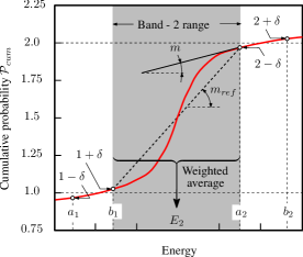
Figure 1: Example of the band determination algorithm. Red solid line (color online): The cumulative probability, $\mathcal{P}_{cum}$, versus energy, shows that Band 2 falls between energies $b_{1}$ ($\mathcal{P}_{cum}=1+\delta$) and $a_{2}$ ($\mathcal{P}_{cum}=2-\delta$), the grey shaded region. The average slope over the step in cumulative probability is $m_{ref}$ (black doted line) and the last $5\%$ of $(E,\mathcal{P}_{cum})$ points in the range are fitted to a line with slope $m$ (solid black line). Because $m<m_{ref}$ the step is distinct and Band 2 can be differentiated from the next higher band(s). The probability-weighted average energy is indicated by $E_{2}$.

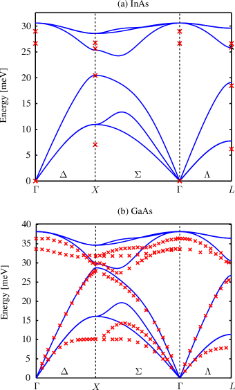
Figure 1: Comparison of the Keating model (solid lines, with parameters given in Table II of the main paper) with experimental data (crosses, from Ref. S_InAs, for InAs and Ref. S_Strauch_JPCM_1990, for GaAs) for the phonon dispersion of (a) InAs and (b) GaAs. Note that the Keating model captures the LA mode in both materials well.

In the modified method, we eliminate the parameters for minimum resolvable gap and minimum probability. Instead, we concentrate on the cumulative probability and its slope. The cumulative probability converges with supercell size (see Sec. III below) and, as we note in connection with electron bands, step determination is simpler than peak determination Boykin et al. (2007b). Our band determination method is given below and illustrated in Fig. 1, where we plot the cumulative probability for fixed PC wavevector $\bm{q}_{m}=\bm{Q}+\bm{G}_{m}$ in the vicinity of the second band edge for an hypothetical system. There are two control parameters: $\delta$ and slopelim. $\delta$ is the difference in the cumulative probability from an integer used to bracket integral values, and slopelim is the cumulative probability slope above which the current candidate band cannot be separated from the next higher one. In practice we have found to $\delta=0.05$ and $\texttt{slopelim}=1.0$ work well. The steps in band determination are:

1. Bracket all integral values, $j$, of the cumulative probability, denoted by the energy ranges $[a_{j},b_{j}]$. That is, $\mathcal{P}_{cum}(a_{j},\bm{q}_{m})=j-\delta$, $\mathcal{P}_{cum}(b_{j},\bm{q}_{m})=j+\delta$. Fig. 1 shows these brackets for $\mathcal{P}_{cum}=1,2$ . The band $(j+1)$ then falls somewhere between energies $b_{j}$ and $a_{j+1}$, as shown in the shaded area of Fig. 1 for band 2. Here band 2 is nondegenerate; degeneracies are treated in Step 3.

2. Next determine whether or not the band in the range $[b_{j},a_{j+1}]$ can be resolved from the next-higher band. Physically, resolution is not possible when the slope of the cumulative probability is too large near the upper end of the range: A rapid increase in the cumulative probability near the upper end of the range means that the current band and the next higher one are for all practical purposes degenerate. We check the slope by fitting a line to the last $5\%$ of points in the range $[b_{j},a_{j+1}]$ and comparing it to the average slope over the entire interval, that of the straight line connecting points $(b_{j},j+\delta)$ and $(a_{j+1},j+1-\delta)$, denoted $m_{ref}$. If

   $$\frac{m}{m_{ref}}>\texttt{slopelim},m_{ref}=\frac{1-2\delta}{a_{j+1}-b_{j}}$$ (28)

   the current band cannot be resolved and it is merged into the next-higher band. In Fig. 1, $m/m_{ref}<\texttt{slopelim}$ and therefore band 2 can be resolved, and its energy is the indicated by the weighted average value, $E_{2}$.

3. Degneracies are characterized by a zero-bracket: This situation occurs when there is no cumulative probability sample satisfying $j-\delta\leq\mathcal{P}_{cum}\leq j+\delta$. (Due to the finite size of the SC the cumulative probability is discrete.) In this case the candidate $j$-th band is merged into a doubly-degenerate band with the $(j+1)$-st and the range under consideration is $[b_{j},a_{j+2}]$. This effective band determination method is applied to the phonon bands of In_xGa_1-xAs in Sec. III below.

Once the bands have been determined, the band energies are computed. Although the dynamical matrix eigenproblem has an eigenvalue $\omega^{2}$, or equivalently $E^{2}$, we continue to compute the average energy as in the electronic structure case Boykin et al. (2007b). Once the range of SC energies contributing to the $j$-th PC band has been found by the procedure above, the PC energy for this band is computed as:

$$\epsilon_{j}(\bm{Q}+\bm{G}_{m})=\dfrac{\sum\limits_{i=M}^{N}\mathcal{P}(E_{i},\bm{Q}+\bm{G}_{m})\cdot E_{i}}{\sum\limits_{i=M}^{N}\mathcal{P}(E_{i},\bm{Q}+\bm{G}_{m})}$$ (29)

where the SC states $i=M,M+1,\ldots,N$ contribute to the $j$-th PC band. The energy range for a set of degenerate bands is determined by Step 3 above and the set’s average energy is computed as in the electronic structure case Boykin et al. (2007b). We note that for strongly peaked functions eq. (29) and a weighted RMS computation over $E^{2}$ will give essentially the same results. More importantly, because the band positions are determined in terms of $E$, not $E^{2}$, eq. (29) is more fully consistent with the band determination method.

III Results

Table 2: Keating Keating (1966) parameters for InAs and GaAs in both Random Alloy and VCA calculations from Ref. Pryor et al., 1998. Units are $N/m$.

	$\alpha$	$\beta$
InAs	$35.18$	$5.49$
GaAs	$41.19$	$8.94$

We demonstrate the effective phonon bandstructure method of Sec. II above by calculating the phonon bands for In_xGa_1-xAs alloys using the Keating model Keating (1966). The parameters for InAs and GaAs Pryor et al. (1998) are listed in Table 2. The Keating model has deficiencies Sui and Herman (1993); Paul et al. (2010); Steiger et al. (2011b); however it does accurately reproduce the longitudinal acoustic (LA) mode from $\Gamma$ to L. The bulk phonon bands for GaAs and InAs reproduced by the Keating model Keating (1966) are included in the supplemental material Supplemental Material for this paper. In the Random Alloy (RA) calculations we use the geometric average of the GaAs and InAs Keating $\beta$ (bond-bending) parameters whenever an As atom is the common nearest-neighbor to both a Ga and an In atom in the bond-pair sum. Otherwise, we use the appropriate bulk parameters for the single bond ($\alpha$) or bond-pair ($\beta$). For the In_0.5Ga_0.5As Virtual Crystal Approximation (VCA) calculations used as a basis for comparison, we employ the geometric average of the respective Keating parameters.

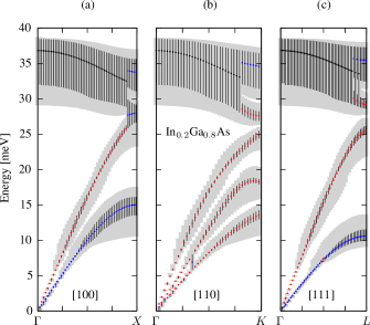
Figure 2: Random Alloy (RA) unfolded bands for In_0.2Ga_0.8As along $[100]$ (a), $[110]$ (b), and $[111]$ (c). Dots indicate average energies and dot color (online) indicates degeneracy, $D$: red (1), blue (2), or black (3). Black lines and grey bars denote the spread in probability for the band they surround: $0.25\leq\mathcal{P}_{band}\leq D-0.25$ (black) or $0.05\leq\mathcal{P}_{band}\leq D-0.05$ (grey).

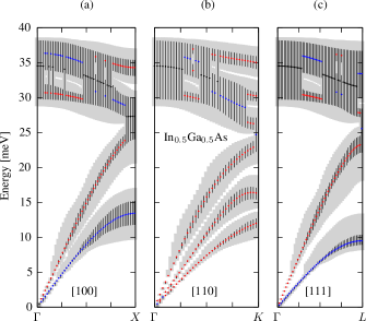
Figure 3: Random Alloy (RA) unfolded bands for In_0.5Ga_0.5As along $[100]$ (a), $[110]$ (b), and $[111]$ (c). The symbols are the same as in Fig. 2.

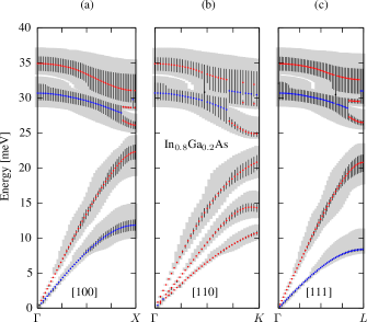
Figure 4: Random Alloy (RA) unfolded bands for In_0.8Ga_0.2As along $[100]$ (a), $[110]$ (b), and $[111]$ (c). The symbols are the same as in Fig. 2.

Figures 2- 4 show the RA unfolded In_xGa_1-xAs bands for $x=0.2$, $0.5$, and $0.8$, respectively, along each of the symmetry directions $[100]$, $[110]$, and $[111]$. The special unit cells for these directions (see Section II.2) are used and in each case, $N_{1}\times N_{2}\times N_{3}=101\times 4\times 4$. As discussed below the bond-length distribution for this size cell was well-converged. In these figures, dots indicate the weighted average energy and dot color (online) denotes the degeneracy, $D$: red (1), blue (2), or black (3). The probability limits on a degenerate band are best expressed in terms of the band probability: For the band falling in the energy range $[b_{j},a_{j+D}]$, $\mathcal{P}_{band}=\mathcal{P}_{cum}-j$. Black lines and grey bars denote the spread in probability for the band they surround: $0.25\leq\mathcal{P}_{band}\leq D-0.25$(black) or $0.05\leq\mathcal{P}_{band}\leq D-0.05$ (grey).

Generally, the acoustic bands are much better resolved than are the optical. This development is not surprising due to the fact that all three optical modes are very close together throughout the Brillouin Zone. Another factor is the large mass discrepancy between the two cations involved, Ga and In. Large mass differences are an unavoidable fact in semiconductor alloys because the alloying process results in replacing an atom by a different one from the same column of the periodic table. The effect on the phonon bands near $q=0$ can be seen in the simple two-atom-per-cell chain model [See; forexample:]Harrison_Book_1979; *Kittel_Book_1996: $\omega_{A}=\sqrt{1/(M_{1}+M_{2})}$, $\omega_{O}=\sqrt{(M_{1}+M_{2})/(M_{1}M_{2})}$. Assuming the same force constant for both materials one finds $\Delta\omega_{A}\Delta\omega_{O}\approx 0.3(qa)$, where $\Delta\omega_{\gamma}=\omega_{\gamma}^{\text{GaAs}}-\omega_{\gamma}^{\text{InAs}}$, $\gamma\in\{A,O\}$. Thus, there are good physical reasons for the greater spreads in the optical versus acoustic modes.

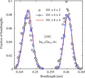
Figure 5: Bondlength convergence test for the $[100]$ In_0.5Ga_0.5As SCs (color online). The SCs use the special $[100]$ PC from Sec. II.B. Three different SC sizes are examined: $101\times 4\times 2$ (black open circles), $101\times 4\times 4$(blue solid line and blue open squares), $101\times 8\times 4$(red solid line). The two largest cells agree well, and therefore we use the $101\times 4\times 4$ SC since it affords accuracy at less computational cost than the $101\times 8\times 4$.

We can gain additional insight into the spreads of the alloy bands by examining the eigenvectors of the simple two-atom chain modelKittel (1996). At $q=0$, the acoustic branch eigenvector is $[1/\sqrt{2},1/\sqrt{2}]^{T}$. In other words, independent of mass and force constant the two atomic displacements have equal magnitudes and are in phase. For the optical mode, the displacements depend on the masses and are of opposite sign (out of phase). This behavior is clear in the RA calculations. In a like manner, the greater spreads near the Brillouin zone boundary in both the acoustic and optical modes of the RA calculations have parallels in the simple two-atom chain at $q=\pi/a$. To make the discussion concrete, assume that atom 1 is As while atom 2 is either Ga or In. In the simple model for $M_{1}>M_{2}$ (GaAs) the acoustic (A) and optical (O) mode eigenvectors are: $\bm{u}_{A}=[1,0]^{T}$, $\bm{u}_{O}=[0,1]^{T}$. In the acoustic mode As is maximally displaced, while Ga is at rest; the optical mode is the opposite. For $M_{1}<M_{2}$ (InAs), these results are exchanged: $\bm{u}_{A}=[0,1]^{T}$, $\bm{u}_{O}=[1,0]^{T}$, so that for the acoustic mode As is stationary and In is maximally displaced, with the optical mode the opposite. Hence there is a serious mismatch between these two materials at $q=\pi/a$ and an increase in the band spread is hardly surprising.

The worst-case alloy, In_0.5Ga_0.5As, is an optimal candidate for further analysis. Fig. 5 shows the bond-length distributions in three different $[100]$ cells, $101\times 4\times 2$, $101\times 4\times 4$, $101\times 8\times 4$. It is clear that the largest two are nearly identical in terms of bond lengths, while the smallest shows significant deviations. Thus, the intermediate cell, $101\times 4\times 4$, can safely be used for calculating alloy dispersions: It offers good accuracy but at a lower computational cost.

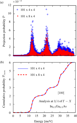
Figure 6: Projection probability (a) and cumulative probability (b) for the $101\times 4\times 4$ (blue open circles and blue solid line, color online) and $101\times 8\times 4$(red solid circles and red dashed line) $[100]$ SCs $75\%$ of the way from $\Gamma$ to $X$ in the PC first Brillouin zone. The cumulative probability has obviously converged, and the projection probability must be lower for the larger cell because the sum rule, eq. 26 fixes the cumulative probability. The larger SC has twice as many samples so each must contribute less due to the fixed cumulative probability.

The reasons for the large uncertainties in the phonon bands become clear when we examine the projection probability and cumulative probability for the $[100]$ In_0.5Ga_0.5As $101\times 4\times 4$ supercell at a specific $\bm{q}$. Figures 6(a,b) show these probabilities $75\%$ of the way from $\Gamma$ to $X$ in the PC first Brillouin zone. While the cumulative probabilities for the two cells are essentially identical the projection probabilities differ. Because the sum rule, eq. (26), fixes the cumulative probability, the projection probability must change when the SC size changes: In the larger SC there are twice as many probability samples so each must contribute less. The twofold degenerate Transverse Acoustic (TA) and singly-degenerate LA modes are well separated in the band plot Fig. 3(a) and this fact is reflected in both Figs. 6(a) and 6(b). In Fig. 6(a) there are two well-defined peaks corresponding to these two modes at around $12$ meV (TA) and $22$ meV (LA). In a like manner the cumulative probability, Fig. 6(b) shows fairly sharp steps up to $2$ between $10-15$ meV and up to $3$ between $20-25$ meV. Above $27$ meV or so, however, Fig. 3(a) show strong mixing of all three optical modes, and this mixing is obvious in both Figs. 6(a) and 6(b). The projection probability, Fig. 6(a), has an ill-defined clump from around $27-38$ meV, and the cumulative probability, Fig. 6(b) has a more or less continuous rise from around $27-38$ meV with little evidence of a pronounced step.

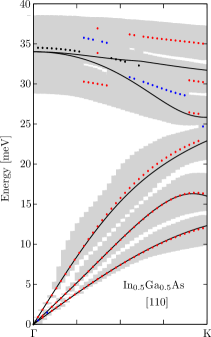
Figure 7: RA and VCA bands for In_0.5Ga_0.5As along $[110]$. The RA bands are represented by dots (color online) and grey bars as in Figs. 2-4. Dots indicate average energies and dot color indicates degeneracy, $D$:red (1), blue (2), or black (3). Grey bars denote the spread in probability for the band they surround: $0.05\leq\mathcal{P}_{band}\leq D-0.05$ . The VCA bands are plotted with black solid lines.

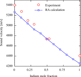
Figure 8: Sound velocity along $[111]$ for In_xGa_1-xAs, computed from $v_{g}=d\omega/dq$ at $q=0$ for the LA mode. Open blue squares (color online) and blue line (as a guide to the eye) are the RA unfolded results while red open circles are the experimental data Wen et al. (2006). There is very good agreement between the RA results and experiment.

In Fig. 7 we compare the VCA and RA bands along $[110]$ for In_0.5Ga_0.5As. The VCA bands are plotted with black lines, the RA results with dots and grey bars as in Figs. 2-4. As seen in 3(b) the acoustic modes are well-defined and the VCA in fact agrees well with the RA results for these modes. The RA optical modes are generally heavily mixed. Both trends have already been discussed with respect to the $[100]$ bands. Although the one-dimensional model is perhaps not quite so direct an analogy in this case (the planes have both anions and cations, while the $[100]$ are exclusively anion or cation), the optical modes are sufficiently close in energy that significant mixing occurs. In contrast, the VCA optical modes remain distinct because in that case the crystal is perfectly ordered.

As mentioned above, the Keating model Keating (1966) does accurately reproduce the acoustic modes from $\Gamma$ to $L$, so that a sound velocity calculation using RA results based on it a good test of the effective phonon bandstructure model presented here. Fig. 8 shows the sound velocity along $[111]$ (i.e., of the LA mode) versus In mole fraction: Open squares and lines (to guide the eye) are the RA results while open circles are experimental results Wen et al. (2006). The $101\times 4\times 4$ $[111]$ SC is used for the RA results, and the sound velocity $v_{g}=dw/dq$ at $q=0$ is calculated with a forward- difference approximation. The uncertainties on the RA calculation are very small so they are not shown: Note the tiny uncertainties for each $[111]$ LA mode near q = 0 in Figures 2-4(c). The RA calculations match the experimental results well with a maximum relative error of under $3\%$. Better agreement could be obtained by using either the modified valence-force-field (MVFF) Sui and Herman (1993); Paul et al. (2010) or enhanced valence-force-field (EVFF) Steiger et al. (2011b) models instead of Keating’s Keating (1966).

IV Conclusions

We have developed an effective phonon bandstructure calculation method based on Brillouin zone unfolding. As in the electronic structure case Boykin et al. (2007b); Boykin and Klimeck (2005); Boykin et al. (2007c) one first randomly populates a SC with the atoms of an alloy in the proper mole fraction, then finds the SC eigenstates. From these, one projects out their contributions to PC states of $\bm{q}_{m}=\bm{Q}+\bm{G}_{m}$ . The probability sum rule for the phonon problem leads to an ansatz for effective band determination: Bands occur at energies where the cumulative probability makes integral steps. We have modified the band determination methodBoykin et al. (2007b); Boykin and Klimeck (2005); Boykin et al. (2007c) to better align it with the different physics of the vibrational spectrum problem. Using this method we have studied the effective phonon bandstructures of In_xGa_1-xAs alloys. In general we find that the optical modes are heavily mixed whereas the acoustic modes tend to be better defined. These characteristics can be at least partly explained by a simple one-dimensional model Kittel (1996). To validate the effective phonon bandstructure method, we calculate the sound velocity along $[111]$ versus mole fraction and find very good agreement with experiment. The method developed here should be useful for thermal problems in transistors, nanotransistors, and other devices made from semiconductor alloys.

*

Appendix A

The special PCs of Sec. II.2 are chosen so as to probe specific parts of the PC Brillouin zone when starting from $\bm{q}=\bm{0}$. For all three cells, we follow the path $\bm{q}:\bm{0}\rightarrow(1/2)\bm{\beta}_{1}^{[lmn]}$ (see Table 1). For the $[100]$ PC, this path is $\Gamma\rightarrow X$, while for the $[111]$ PC, it is $\Gamma\rightarrow L$. For the $[110]$ cell, this path crosses the Brillouin zone boundary at $(3/8)\bm{\beta}_{1}^{[110]}$, so the first three-fourths of the path corresponds to $\Gamma\rightarrow K$. The last quarter, $\bm{q}:(3/8)\bm{\beta}_{1}^{[110]}\rightarrow(1/2)\bm{\beta}_{1}^{[110]}$ is easily shifted back into the first Brillouin zone by adding the reciprocal lattice vector $\bm{\beta}_{2}^{[110]}$. After shifting, the remainder now traverses the top diamond from the side midpoint to its center, $U\rightarrow X$ . Here we only plot the bands for the $\Gamma\rightarrow K$ portion of the path since it is of the most interest.

Supplemental Material : Brillouin zone unfolding method for effective phonon spectra

1. Keating model for InAs and GaAs

2. Convergence with supercell size

Fig. 6 of the main paper shows the convergence of the cumulative probability for the $101\times 4\times 4$ and $101\times 8\times 4$ supercells at a point $75\%$ of the distance from $\Gamma\rightarrow X$. Fig. 2 below shows the final effective bandstructure obtained from these two supercells. Note the good convergence of the effective bandstructure with supercell size. The differences seen w.r.t the position of the mean and the spread in the optical bands are artifacts of the slope condition (eq. 28) of the band determination algorithm. As pointed out in the discussion connected to Fig. 6 of the main paper, the optical bands are strongly mixed. Hence, there are cases where the slope condition is just about satisfied. In these cases, even small differences in cumulative probability with lead to different binning of energies, and their consequent mean and spread. Nevertheless, note that the degeneracies are reported in a consistent manner.

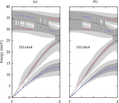
Figure 2: Convergence of the effective bandstructure with supercell size, shown for In_0.5Ga_0.5As along the $[100]$ direction. The symbols are the same as in Fig. 2 of the main paper.

3. Comparison of effective bandstructure along equivalent directions in the Brillouin zone

A perfect crystal can have several equivalent directions in the Brillouin zone, based on its symmetry. By definition, a random alloy has no such equivalent directions. Nevertheless, if the individual constituents of an alloy belong to the same symmetry class (like for example, InAs and GaAs), we would like the effective unfolded bandstructure to manifest this symmetry. Ref. S_Zunger_PRB_2012, achieves this by averaging the cumulative probability over these equivalent directions, prior to constructing an effective bandstructure. We do not perform this averaging in this work. However, we do not expect the final result of such an averaging to be significantly different from the results obtained from considering only one of the many equivalent directions. For example, Fig. 3 above shows the effective bandstructure of In_0.5Ga_0.5As along the $[111]$ and $[1\bar{1}1]$ directions, computed using $101\times 4\times 4$ supercells. The supercell for the $[111]$ direction is constructed as before, using the primitve cell lattice vectors given in Table I of the main paper. The supercell for the $[1\bar{1}1]$ direction uses $\alpha_{1}=(1,0,1),\alpha_{2}=(0,1,1),\alpha_{3}=(-1,-1,0)$ (specified as earlier, in cartesian coordinates and units of $a/2$). The effective bandstructure indeed looks very similar for these directions (the small differences w.r.t mean and spread in the optical bands are due to the reason described in the previous section).

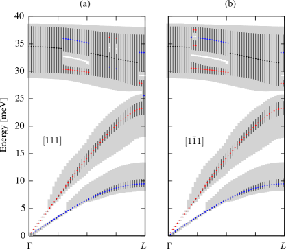
Figure 3: Comparison of the effective bandstructure along equivalent directions in the Brillouin zone, shown for In_0.5Ga_0.5As along the $[111]$ and $[1\bar{1}1]$ directions. Calculations were performed using $101\times 4\times 4$ supercells. The symbols are the same as in Fig. 2 of the main paper.

4. Effective bandstructure of In_xGa_1-xAs for $x=\mathbf{0.0,0.1,\ldots 1.0}$

For completeness, we present the computed bandstructure of In_xGa_1-xAs for $x=0.0,0.1,$ $\ldots 1.0$ in Figs. 4-14 below. Note that Figs. 2-4 of the main paper present the effective phonon bandstructure of In_0.2Ga_0.8As, In_0.5Ga_0.5As and In_0.8Ga_0.2As respectively, but are nevertheless repeated here. All computations used the $101\times 4\times 4$ supercell.

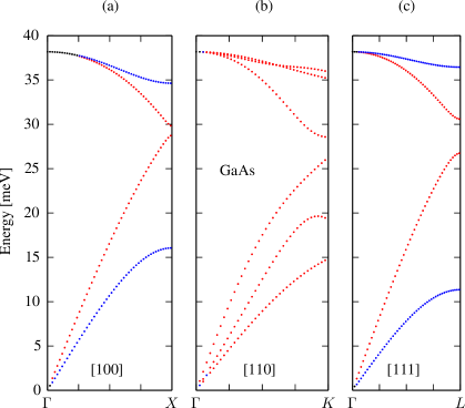
Figure 4: Unfolded bands for GaAs along $[100]$ (a), $[110]$ (b), and $[111]$ (c). The symbols are the same as in Fig. 2 of the main paper.

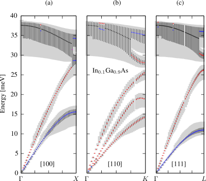
Figure 5: Random Alloy (RA) unfolded bands for In_0.1Ga_0.9As along $[100]$ (a), $[110]$ (b), and $[111]$ (c). The symbols are the same as in Fig. 2 of the main paper.

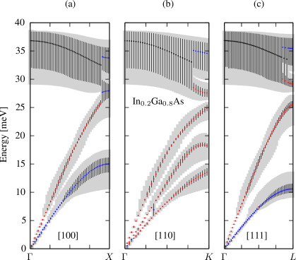
Figure 6: Random Alloy (RA) unfolded bands for In_0.2Ga_0.8As along $[100]$ (a), $[110]$ (b), and $[111]$ (c). The symbols are the same as in Fig. 2 of the main paper.

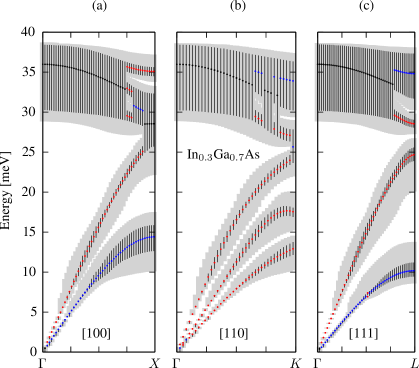
Figure 7: Random Alloy (RA) unfolded bands for In_0.3Ga_0.7As along $[100]$ (a), $[110]$ (b), and $[111]$ (c). The symbols are the same as in Fig. 2 of the main paper.

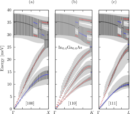
Figure 8: Random Alloy (RA) unfolded bands for In_0.4Ga_0.6As along $[100]$ (a), $[110]$ (b), and $[111]$ (c). The symbols are the same as in Fig. 2 of the main paper.

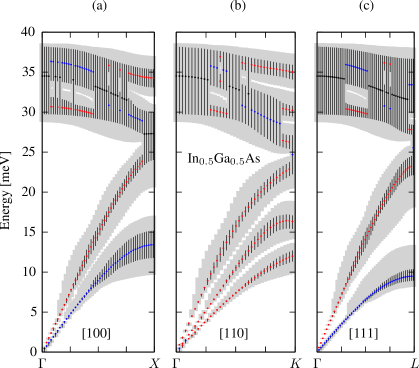
Figure 9: Random Alloy (RA) unfolded bands for In_0.5Ga_0.5As along $[100]$ (a), $[110]$ (b), and $[111]$ (c). The symbols are the same as in Fig. 2 of the main paper.

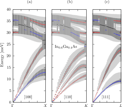
Figure 10: Random Alloy (RA) unfolded bands for In_0.6Ga_0.4As along $[100]$ (a), $[110]$ (b), and $[111]$ (c). The symbols are the same as in Fig. 2 of the main paper.

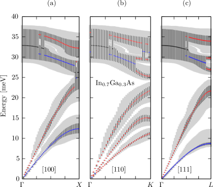
Figure 11: Random Alloy (RA) unfolded bands for In_0.7Ga_0.3As along $[100]$ (a), $[110]$ (b), and $[111]$ (c). The symbols are the same as in Fig. 2 of the main paper.

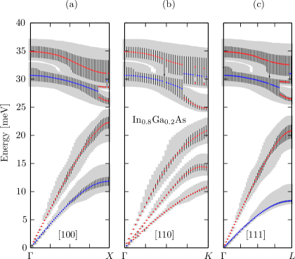
Figure 12: Random Alloy (RA) unfolded bands for In_0.8Ga_0.2As along $[100]$ (a), $[110]$ (b), and $[111]$ (c). The symbols are the same as in Fig. 2 of the main paper.

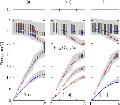
Figure 13: Random Alloy (RA) unfolded bands for In_0.9Ga_0.1As along $[100]$ (a), $[110]$ (b), and $[111]$ (c). The symbols are the same as in Fig. 2 of the main paper.

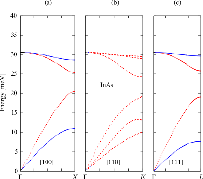
Figure 14: Unfolded bands for InAs along $[100]$ (a), $[110]$ (b), and $[111]$ (c). The symbols are the same as in Fig. 2 of the main paper.

References

- Duan et al. (2001) X. Duan, Y. Huang, Y. Cui, J. Wang, and C. M. Lieber, Nature 409, 66 (2001).
- Persson et al. (2006) A. Persson, M. Björk, S. Jeppesen, J. Wagner, L. Wallenberg, and L. Samuelson, Nano Lett. 6, 403 (2006).
- Vandecasteele et al. (2009) N. Vandecasteele, M. Lazzeri, and F. Mauri, Phys. Rev. Lett. 102, 196801 (2009).
- Khurgin et al. (2008) J. B. Khurgin, D. Jena, and Y. J. Ding, Appl. Phys. Lett. 93, 032110 (2008).
- Boykin et al. (2007a) T. B. Boykin, M. Luisier, A. Schenk, N. Kharche, and G. Klimeck, IEEE Trans. Nanotechnol. 6, 43 (2007a).
- Kharche et al. (2008) N. Kharche, M. Luisier, T. B. Boykin, and G. Klimeck, J. Comp. Electron. 7, 350 (2008).
- Salmani-Jelodar et al. (2012) M. Salmani-Jelodar, A. Paul, T. Boykin, and G. Klimeck, J. Comp. Electron. 11, 22 (2012).
- Boykin et al. (2007b) T. B. Boykin, N. Kharche, G. Klimeck, and M. Korkusinski, J. Phys: Condens. Matter 19, 036203 (2007b).
- Boykin and Klimeck (2005) T. B. Boykin and G. Klimeck, Phys. Rev. B 71, 115215 (2005).
- Boykin et al. (2007c) T. B. Boykin, N. Kharche, and G. Klimeck, Phys. Rev. B 76, 035310 (2007c).
- Popescu and Zunger (2010) V. Popescu and A. Zunger, Phys. Rev. Lett. 104, 236403 (2010).
- Popescu and Zunger (2012) V. Popescu and A. Zunger, Phys. Rev. B 85, 085201 (2012).
- Ajoy et al. (2012) A. Ajoy, K. V. Murali, and S. Karmalkar, J. Phys.: Condens. Matter 24, 055504 (2012).
- Allen et al. (2013a) P. B. Allen, T. Berlijn, D. Casavant, and J. Soler, Phys. Rev. B 87, 085322 (2013a).
- Allen et al. (2013b) P. Allen, T. Berlijn, D. Casavant, and J. Soler, Phys. Rev. B 87, 239904 (2013b).
- Ku et al. (2010) W. Ku, T. Berlijn, and C.-C. Lee, Phys. Rev. Lett. 104, 216401 (2010).
- Berlijn (2014) T. Berlijn, Phys. Rev. B 89, 104511 (2014).
- Lee et al. (2013) C.-C. Lee, Y. Yamada-Takamura, and T. Ozaki, J. Phys.: Condens. Matter 25, 345501 (2013).
- Huang et al. (2014) H. Huang, F. Zheng, P. Zhang, J. Wu, B.-L. Gu, and W. Duan, New J. Phys. 16, 033034 (2014).
- Medeiros et al. (2014) P. V. Medeiros, S. Stafström, and J. Björk, Phys. Rev. B 89, 041407 (2014).
- Peil et al. (2012) O. E. Peil, A. V. Ruban, and B. Johansson, Phys. Rev. B 85, 165140 (2012).
- Wang et al. (2011) Y. Wang, C. L. Zacherl, S. Shang, L.-Q. Chen, and Z.-K. Liu, J. Phys.: Condens. Matter 23, 485403 (2011).
- Boykin et al. (2009) T. B. Boykin, N. Kharche, and G. Klimeck, Physica E 41, 490 (2009).
- Steiger et al. (2011a) S. Steiger, M. Povolotskyi, H.-H. Park, T. Kubis, and G. Klimeck, IEEE Trans. Nanotechnol. 10, 1464 (2011a).
- Fonseca et al. (2013) J. Fonseca, T. Kubis, M. Povolotskyi, B. Novakovic, A. Ajoy, G. Hegde, H. Ilatikhameneh, Z. Jiang, P. Sengupta, Y. Tan, et al., J. Comp. Electron. 12, 592 (2013).
- Aravind (2006) P. Aravind, Am. J. Phys. 74, 794 (2006).
- Madelung (1981) O. Madelung, “Introduction to solid-state theory,” (Springer, 1981) Chap. 3.3.
- Keating (1966) P. Keating, Phys. Rev. 145, 637 (1966).
- Pryor et al. (1998) C. Pryor, J. Kim, L. Wang, A. Williamson, and A. Zunger, J. Appl. Phys. 83, 2548 (1998).
- Sui and Herman (1993) Z. Sui and I. P. Herman, Phys. Rev. B 48, 17938 (1993).
- Paul et al. (2010) A. Paul, M. Luisier, and G. Klimeck, J. Comp. Electron. 9, 160 (2010).
- Steiger et al. (2011b) S. Steiger, M. Salmani-Jelodar, D. Areshkin, A. Paul, T. Kubis, M. Povolotskyi, H.-H. Park, and G. Klimeck, Phys. Rev. B 84, 155204 (2011b).
- (33) Supplemental Material.
- Harrison (1979) W. A. Harrison, “Solid State Theory,” (Dover New York, 1979) Chap. IV.
- Kittel (1996) C. Kittel, “Introduction to Solid State Physics,” (Wiley New York, 1996) Chap. 4, 7th ed.
- Wen et al. (2006) Y.-C. Wen, L.-C. Chou, H.-H. Lin, K.-H. Lin, T.-F. Kao, and C.-K. Sun, J. Appl. Phys. 100, 103516 (2006).

References

- (1) http://www.ioffe.ru/SVA/NSM/Semicond/InAs/mechanic.html#phonon.
- (2) D. Strauch and B. Dorner, “Phonon dispersion in GaAs,” J. Physics: Condens. Matter, vol. 2, no. 6, p. 1457, 1990.
- (3) V. Popescu and A. Zunger, “Extracting E versus k effective band structure from supercell calculations on alloys and impurities,” Phys. Rev. B, vol. 85, no. 8, p. 085201, 2012.